Article

Generation of Surface Maps of Erosion Resistance for Wind Turbine Blades under Rain Flows

by
Alessio Castorrini
1,*,
Paolo Venturini
2 and
Aldo Bonfiglioli
1
1
School of Engineering, Università della Basilicata, Viale dell’Ateneo Lucano 10, 85100 Potenza, Italy
2
Department of Mechanical and Aerospace Engineering, Sapienza University of Rome, Via Eudossiana 18, 00184 Rome, Italy
*
Author to whom correspondence should be addressed.
Energies 2022, 15(15), 5593; https://doi.org/10.3390/en15155593
Submission received: 12 July 2022 / Revised: 28 July 2022 / Accepted: 29 July 2022 / Published: 2 August 2022
(This article belongs to the Special Issue Wind Turbine Advances)

Abstract

:
Rain erosion on wind turbine blades raises considerable interest in wind energy industry and research, and the definition of accurate erosion prediction systems can facilitate a rapid development of solutions for blade protection. We propose here the application of a novel methodology able to integrate a multibody aeroelastic simulation of the whole wind turbine, based on engineering models, with high-fidelity simulations of aerodynamics and particle transport and with semi-empirical models for the prediction of the damage incubation time. This methodology is applied to generate a parametric map of the blade regions potentially affected by erosion in terms of the fatigue life of the coating surface. This map can represent an important reference for the evaluation of the sustainability of maintenance, control and mitigation interventions.

1. Introduction

The concern about climate change is pushing countries all over the world to transform energy production processes from fossil-fuel-based to renewable-source-based. The COP26 meeting held in Glasgow (UK), November 2021 [1], reaffirmed the goal fixed in the Paris Agreement [2] of holding the increase in the global average temperature under 2 °C above pre-industrial levels and pursuing efforts to limit the temperature increase to 1.5 °C above pre-industrial levels. This requires a quick response by the governments trying to reduce CO 2 emissions by 45% by 2030 relative to the 2010 levels and to net zero by 2050. To reach the goal, about 37 Gt/yr of CO 2 should be cut by 2050. According to the International Renewable Energy Agency [3], this can be achieved, beside other measures, through a strong increase in renewable electricity production, with solar and wind energies being the leaders of such a transformation because they are the most convenient technologies and those with the greatest development potential. By 2030, the world onshore installed capacity should reach about 3000 GW (4 times that of 2020) and the offshore one about 380 GW (11 times that of 2020). This implies a big effort to increase not only the number of installed wind turbines but also their rotor diameter, and these are exactly the directions that manufacturers and wind farm managers have been following for some time. In fact, in recent years, there has been a strong increase in wind energy installed power: in 2000, the world installed capacity was about 18 GW, and in 2019, it was more than 650 GW and 840 GW in 2021, with 59 GW installed in 2019, 92.7 GW in 2020 and 97.3 GW in 2021 [4]. At the same time, as reported in the open literature (i.e., [5,6,7,8]), wind turbine sizes are continuously growing (10 MW offshore wind turbines have been available on the market since 2019, having about a 165 m rotor diameter). This leads to tip speeds larger than 100 m/s. Such a high velocity increases rain-, hailstone- and sand-related erosion issues, leading to a fast deterioration of the blades. Focusing the attention on rain erosion, it is clear that if not properly treated, this phenomenon can provoke losses of annual energy production (typically between 1 and 5% [9]) and blade damages, with consequent maintenance and replacement costs. Dalili et al. [10] and Rempel [11] reported that, in some wind farms, severe leading edge erosion signs were found after just two to three years of operations. In 2016, all the 273 blades of the Horns Rev 2 offshore wind farm were refurbished after less than seven years of operations due to severe erosion [12]. In 2018, just after five years of operation, unexpected blade repair due to severe erosion was performed on 140 of the 175 wind turbines in the London Array wind farm. The same was done in the Anholt (Denmark) wind farm, with 87 wind turbines removed out of 111 [13]. Possible solutions to this problem include the maintenance and repair of damage [14], the use of shielding [13] or the control of the turbine in such a way as to limit its speed during intense events (an erosion-safe operational mode) [15]. Each of these interventions is associated with a direct cost related to the operation and materials and an indirect cost related to periods of downtime or operation at reduced efficiency of the power plant. The planning of the best strategy that a wind farm operator can apply, minimizing the revenue losses associated with the rain erosion of the blades, requires an in-depth knowledge of the phenomenon and its impact on the machines. The present research aims at developing a methodology for predicting the time that a blade can operate under realistic weather conditions before erosion starts.
Many studies of WT blade erosion appeared in the last years, confirming a growing interest in the wind energy sector on this issue. Topics of interest include: the coating response to impinging droplets [12,16], the effect of wind speed, droplet size and density on the erosion of wind turbine sections with computational methods [17] and experiments in whirling arm or water-jet facilities (e.g., [18]). These results improve the understanding of rain erosion mechanisms on blade-coating materials, and they constitute a solid background for the definition and validation of empirical methods for erosion computation. In particular, we can identify from the literature two classes of methods for the prediction of the erosion incubation. A first group is based on semi-empirical models, such as the one proposed by Springer [19], which provides a formula to evaluate the number of impacts of erosion incubation. The second group of methods involves the computation of the stress induced by the individual impact of droplets of different sizes, using it to estimate the fatigue damage in the coating material, e.g., by using the Palmgren–Miner’s rule [20]. It is possible to find a comprehensive review of these methods in [21].
Focusing on numerical methods, the authors’ research group carried out an extensive activity devoted to the development of methods to predict the erosion of wind turbine blades that fits into this fast-moving context. The work presented in [22] defined an approach to evaluate the severity of rain erosion damage in multi-MW wind turbines, based on the water-hammer pressure exerted during rain droplet impacts. In [23], the mass and thickness of the material removed from a wind turbine blade due to rain erosion was computed using CFD and particle cloud tracking methods developed by the authors. In [24], an algorithm for performing CFD simulations of long-time erosion processes accounting for the geometry modification of the blade was presented, defining appropriate scale factors to simulate years of operating conditions. In the latest works ([25,26]), a numerical prediction tool coupling CFD simulations with a machine learning approach was defined to predict rain erosion damage on a blade profile. This research represents a first and unique example of merging between rain erosion models, computational fluid and particles dynamics and wind turbine simulation over a full range of realistic operating conditions.
In this paper, we present the application of the technology defined in [26] to carry out a systematic study on the prediction of the erosion incubation period over the surface of a 5MW wind turbine blade, defining the methodology to obtain the measure and build up a comprehensive surface map to use along with the statistics of rain and wind associated to a given installation site. The paper is then structured as follows. The first section describes the methodology in terms of (i) the extension of the original model of [26] in order to measure the erosion incubation period and (ii) the verification and tuning of Springer’s erosion model using rain erosion test data. The second section presents the particular application in the study and the wind turbine blade model and installation site characteristics. Finally, Section 3 presents the results in terms of the damage incubation map over the set of the sample blade sections and its application to obtain the blade surface erosion resistance after a year of operation at the site, with the rain and wind characteristics defined in Section 2.3. Some remarks close the paper.

2. Materials and Methods

The basis for the methodology and the model adopted in this study has been given in [25,26]. In this work, we propose a further extension and specialization to create a map of the erosion incubation time on the blade surface (i.e., the time until the coating material breaks). In Section 2.1, we summarize the main algorithm defined for the study and the details of the new models used to extend the original formulation. Section 2.2 reports a validation study of the method along with the tuning of the erosion model based on whirling arm experiments. The sample application used to demonstrate the technology is described in Section 2.3.

2.1. Methodology

The objective of the proposed methodology is the following: given a wind turbine blade and an installation site, to draw up an accurate map of the areas of the blade that could be affected by rain erosion and the time needed before removal of the material from the blade occurs (i.e., the incubation period).
We start by defining a way to quantify the vulnerability of the blade-coating material to droplet erosion. We rely on classical models of erosion by liquid particles (e.g., [19]), in which three regimes of interaction between material and impacting particles are usually identified. The first regime is called i n c u b a t i o n , where the energy of the impinging droplets is absorbed by the coating without removal of material. After the repetition of a certain number of impact cycles, the material is brought to fatigue failure; at this point, the material removal regime begins, which is generally characterized by a constant erosion rate (i.e., the volume of removed material increases linearly with the number of impacts). After a second threshold of impact cycles, the removal rate decreases, following a different linear trend at a lower slope. Springer’s model [19] is one of the most widely used erosion models for predicting rain erosion on wind turbines. This model predicts that, given specific material and droplet impact characteristics (in terms of size, angle and impact velocity), it is possible to obtain by an empirical correlation the value of the number of incubation impacts per unit area ( n p ) t h r , i.e., the number of impacts per squared meter (1/m 2 ) of that droplet class necessary to start erosion of the material:
( n p ) t h r = 1 A p p a 1 S e f f σ 0 ¯ a 2
where A p p is the projected area of the droplet, S e f f is a reference stress depending on the coating strength, σ 0 ¯ is a reference stress relative to the impacting droplets and a 1 , a 2 are empirical constants [19].
Measuring in a given time T, the number of impacts per unit area for a given class i, characterized by drops of the same size and speed ( n i ), we can obtain the incubation time by reverting the fatigue damage formula n i / ( n p ) t h r = 1 / T . In this work, we will use hours as time units.
Nevertheless, it should be noted that for wind turbine blades operating under real conditions, even assuming the same material for the entire blade surface, impact events will be various and dependent on: geometrical factors (position of the impact point on the aerodynamic surface), climatic factors (variability of the mean wind profile and turbulence, variability of droplet size and concentration, variability of rain intensity) and machine operational factors (blade pitch and rotation speed, control laws, elasticity, azimuthal position, yaw, floating platform motion, etc.). In the present contribution, we follow Palmgren–Miner’s criterion, identifying the incubation period as the time at which the sum of all terms n i / ( n p ) t h r for every class of impact i affecting the material at a given point gives 1. Following this reasoning, let x be a point on the blade surface, assuming a reference period for measuring impacts n i of 1 h, we obtain the map of the incubation period in hours on the surface of the blade via the formula:
T t h r ( x ) = i = 1 N i n i ( x ) ( n p ) t h r ( x ) 1
At this point the challenge is to realistically model all N i possible impact conditions in terms of n i and ( n p ) t h r for any point on the surface, taking into account the previously mentioned variability factors. The solution paradigm to this problem follows what was already defined and demonstrated in [25,26].
First, the airfoils representing the sections of the blade aerodynamic surface are identified. Then, for a given airfoil and for a given flow of n T O T drops per unit surface, a metamodel is generated to define the function:
{ n p , V p , θ } = F ( s , α , R e , d p )
where s is a curvilinear abscissa identifying a point along the airfoil line, starting from the trailing edge on the suction side and ending at the trailing edge on the pressure side (see Figure 1). α is the aerodynamic angle of attack and R e the Reynolds number of the relative flow, d p the diameter of the spherical particles carried by the relative flow, n p the number of impacts per unit target area, θ and V p the angle and velocity of impact of the particles at point s. As reported in detail in [25,26], the F function is obtained through the application of a machine learning algorithm trained on a database of CFD and particle-tracking simulations of the same airfoil, performed for a wide range of angles of attack, Reynolds numbers and particle sizes. The airfoils define the blade sections taken at a discrete set of radial locations along the span. For each section, the airfoil is scaled by the local chord length and rotated by the local twist angle, both given by the definition of the blade surface design. By using this transformation, it is possible to pass from the local curvilinear point s of the airfoil to the corresponding point x on the 3D blade. It follows that the span-wise resolution of the method directly depends on the number of sections used to discretize the blade. By doing so, we are able to obtain the distribution of impact variables needed to define n i and ( n p ) t h r .
The method implies to discretize the blade into slices with 2D symmetry (blade elements) but also being able to provide the F function with the aerodynamic conditions and particle flux of the relative current associated with each slice. This is possible, for example, by using engineering codes that simulate the whole machine by modeling aerodynamics using the blade element theory, the elasticity of the main mechanical components with one-dimensional models, then taking into account the rigid motions of all the elements of the system subject to loads and control laws. In this work, we use openfast [27] for the wind turbine simulation, from which it is possible to extract the instantaneous relative velocity for each blade element involved in our analysis. With this tool, it is possible to take into account the variability related to the operational factors of the machine.
The wind variability will be considered by setting up a set of openfast simulations in which the machine operates under wind inflows with fixed average velocity, a vertical velocity profile and velocity fluctuations in space and time associated to the turbulence. The wind, for each mean velocity condition, is generated with turbsim [28], applying the power law with exponent 1/7 for the vertical velocity profile and the Kaimal model for the stochastic generation of the fluctuations. The simulation time is selected to ensure sufficient convergence of the load and wind averages, in particular, each simulation will be run for 10 min, while the result is recorded every 0.1 s, for a total of N t records. The number of simulations performed for a blade is given by a set of N V mean wind speeds V, which defines the range of the operating velocity of the machine V c u t i n < V < V c u t o u t with interval Δ V of 1 m/s. This automatically defines a matrix of N v × N t conditions simulated for each blade element.
It remains to properly model the variability of the rain. We decided to do this through the rain flow intensity parameter R h , measuring the amount of rain (in mm) falling in one square meter in an hour. Dense literature can be found to also define the statistical correlation between rain flow intensity and droplet size [29]. We adopt the description given by [30], based on the model defined in [31]. Considering this model, we can apply the following probability density function f h to account for the droplet diameter d p variability for a given average R h of the rain events in the site:
f h ( d p , R h ) = 17.67 d p 0.67 2.25 d p d p 1.3 R h 0.232 2.25 exp d p 1.3 R h 0.232 2.25 ;
We then define a set of simulations where the rain intensity V R F varies (5, 10, 15 and 20 mm/h). In all the simulations, we set a maximum size of the droplets of 3 mm, because the droplet size could fall far from the bounds of training database, but also because for diameters greater than 3 mm, the particle shape is not anymore spherical ([32]), and its probability to split into smaller drops increases. Figure 2 reports the probability density function of the raindrop sizes for the selected cases, calculated according to [30].
We aim to present a result that is as general as possible. Because there is no precise relationship between wind speed and rainflow, and because this relationship can be determined by means of measurements and site analyses, we will generate erosion incubation maps that are specific to a given average wind speed (taken over the operating range) and to a given rainflow rate. The matrix of maps obtained for all velocity and rainflow conditions under consideration can then be used via the principle of superposition (Equation (3) is a sum of terms) once the wind and rainflow statistics and correlations for a specific site have been established. An example will be presented in Section 3.
Finally, we can define the generic map of the hours required to initiate erosion on the points x of the surface of a wind blade hit by rain of intensity R h at a given average operating speed of the machine as:
T t h r ( V , R h ) ( x ) = t = 1 N t min ( d p ) max ( d p ) F A C T n p 1 π ( ϕ / 2 ) 2 a 1 S e f f σ 0 ¯ ( V p , θ ) a 2 d ϕ 1
Let us note how for each record t of the dynamic simulation at average speed V, and for each possible diameter of the drops d p , a particular impact pattern is defined, being n p , V p , θ and thus σ 0 ¯ , dependent on the value measured at t of α , R e and d p , by the function F . It remains to define the scale factor that returns the number of impacting droplets n i , from the one resulting from the function F , i.e., n p , which is normalized and relative to the number of particles simulated in the training database n T O T , to the number actually impacting at t. In particular, we define the scale factor for this application as:
F A C T = f h ( d p ) n R n T O T T R T S I M 1 N t
where n R is the total amount of droplets per unit surface fallen in the reference time period T R = 1 h, n T O T is the total amount of droplet injected in the database particle-tracking simulations and T S I M = N t s t e p s Δ t * .

2.2. Erosion Model Tuning
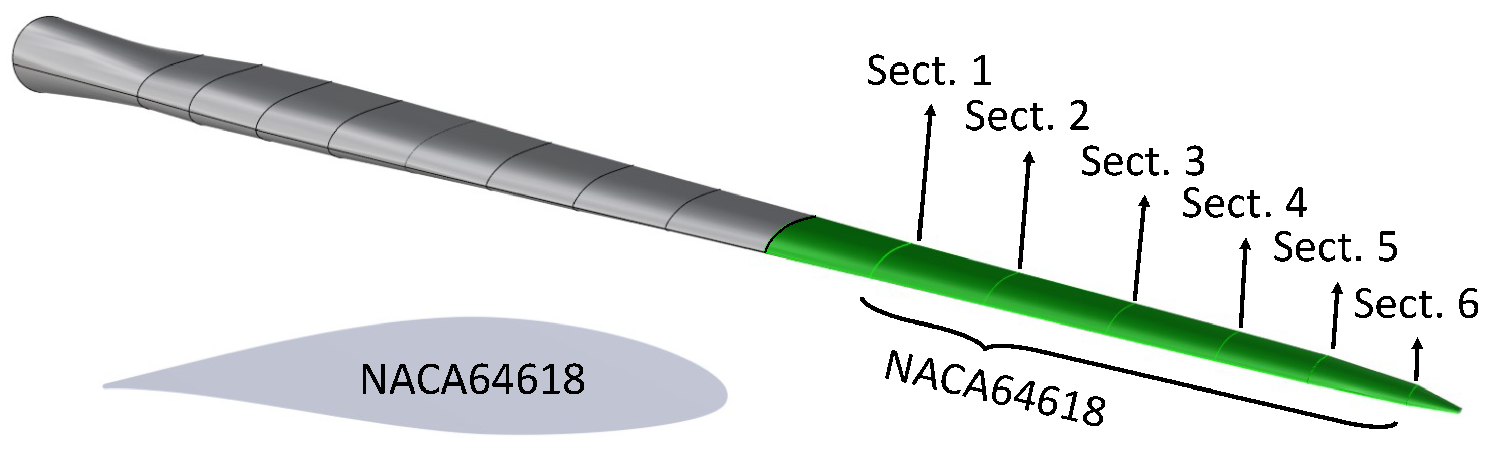
In order to verify and tune Springer’s model [19], here adopted for predicting erosion on blade sections, we refer to the experiments reported in [18]. In that work, O’Carroll et al. measured the incubation period of a set of specimens made of different polymeric materials used in wind blade construction, exposed to the impacts of liquid droplets. From [18], we select the polymethyl methacrylate (PMMA)-based materials, both extruded (PMMA-E) and cast (PMMA-C); their characteristics are reported in Table 1. All these characteristics are reported in [18]. Values of Poisson’s ratio for the tested materials are not shown in the reference study; thus, in the tuning procedure we performed to calibrate the Springer’s model constants, we also included this quantity to be calibrated with the constraint to keep it within the range found in the literature and available on the market (see Table 1 for references). Because the experiments in [18] are performed in an accelerated erosion test bench, it is important to convert the results (expressed in minutes) into real time. To do this, knowing the equivalent rainfall rate of the tests (25.0 mm/h), the specimen size (27.0 × 27.0 mm), the average droplet diameters (2.0 mm), the impact velocity (135.0 m/s) and the incubation time for each material, we could compute the amount of water hitting a specimen during the incubation period, and therefore the number of droplets per unit surface. This quantity was then used to tune the erosion model.
The incubation period measured for the tested materials is reported in Table 2, together with the respective values of Poisson’s ratio and a 2 (Springer’s model constant) provided by the optimization procedure. By using such values for the respective materials, Springer’s model can be tuned and then used to compute the incubation period of any droplet size class. Then, as explained in Section 2.1, the Palmgren–Miner’s rule allows to predict the incubation period in any kind of application, rain size and intensity.

2.3. Test Case

The blade chosen for the test case is that of the 5MW baseline wind turbine defined by the National Renewable Energy Laboratory (NREL) [42]. Table 3 reports the blade elements data in terms of airfoils, chord and twist, identifying also the blade elements used in this study for the generation of the erosion incubation results. In particular, we select 6 sections in the outboard portion of the blade (from 70% of its span to the last section before the blade tip). Figure 3 shows a view of the blade surface, identifying the sections used in this test, the blade surface interested in the generation of the erosion incubation map and the shape of the airfoil defining these sections.
The erosion incubation maps can be combined with annual statistics of wind velocity and rain intensity for a given site of interest in order to obtain a site-specific prediction of the incubation time. According to Verma et al. [43], we can define a probability density function for the rain intensity based on the log-normal distribution:
f R h ( R h ) = 1 2 π σ 2 exp ( ln ( R h ) μ ) 2 2 σ 2 ,
where we assume μ = 1.0 mm/h and σ = 0.2 mm/h.
The Weibull distribution is often used to characterize the probability density function of the wind velocity as it provides a good fit with measured wind data. Therefore, we can define the wind velocity PDF as
f V ( V ) = k c V c k 1 exp V c k ,
where we will assume a shape factor k = 2 and a scale factor c = 9 . Figure 4 shows the probability density functions selected to characterize the wind and rain intensity at installation site.
Then, similarly to what was proposed in [43] and according to Equation (2), we can obtain the incubation period in hours, for any given point x on the blade surface, using the following integration:
T t h r ( x ) = i j n i ( x , V ( i ) , R h ( j ) ) ( n p ) t h r ( x , V ( i ) , R h ( j ) ) f R h ( R h ( j ) ) f V ( V ( i ) ) Δ R h Δ V 1
where, in this sample application, Δ V = 1 m/s and Δ R h = 5 mm/h.

3. Results

This section reports the results and the discussion, first, about the erosion incubation damage maps generated for the blade sections and materials selected in Section 2.1 and, last, about the result of the application of this map to integrate the total incubation period estimated for a given installation site. The results will be presented in terms of the variation of the variable n i / ( n p ) t h r and T t h r , along the airfoil normalized coordinate s defined as in Figure 1.

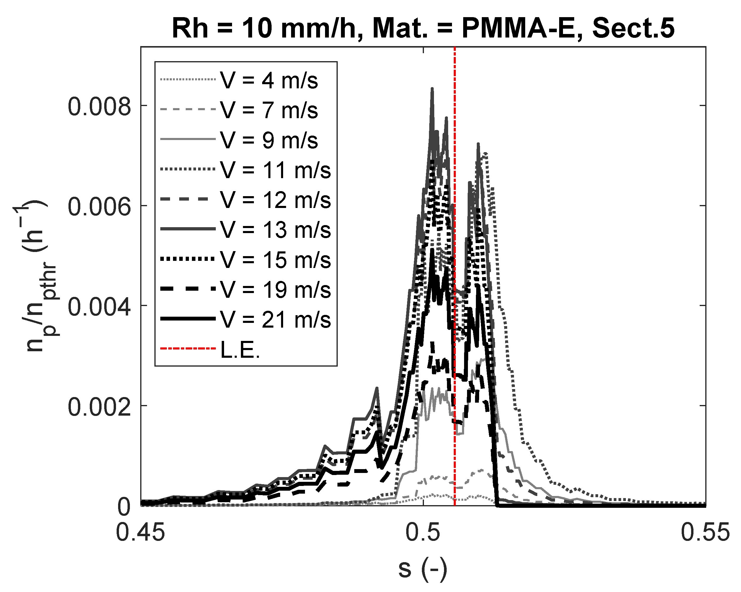
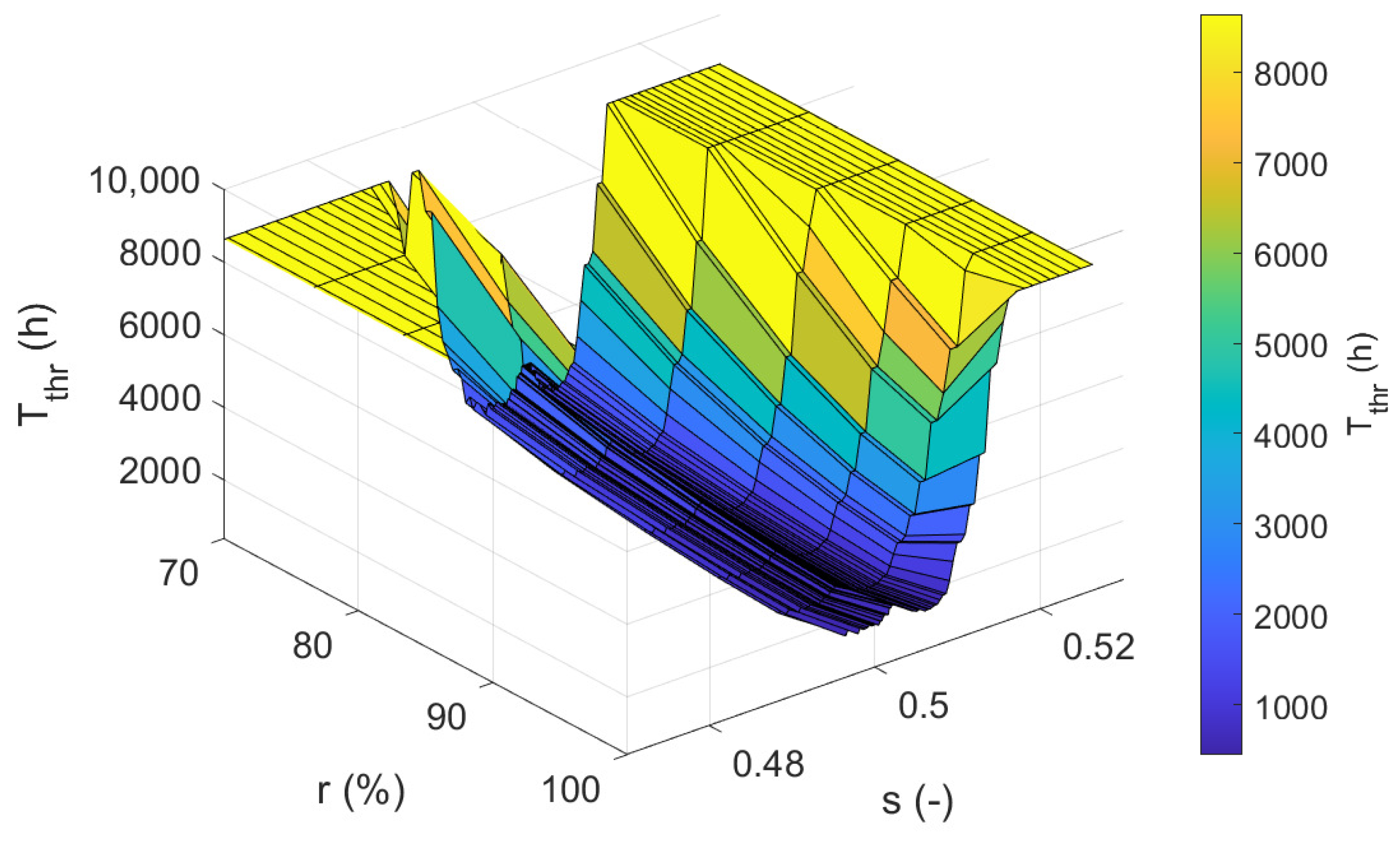
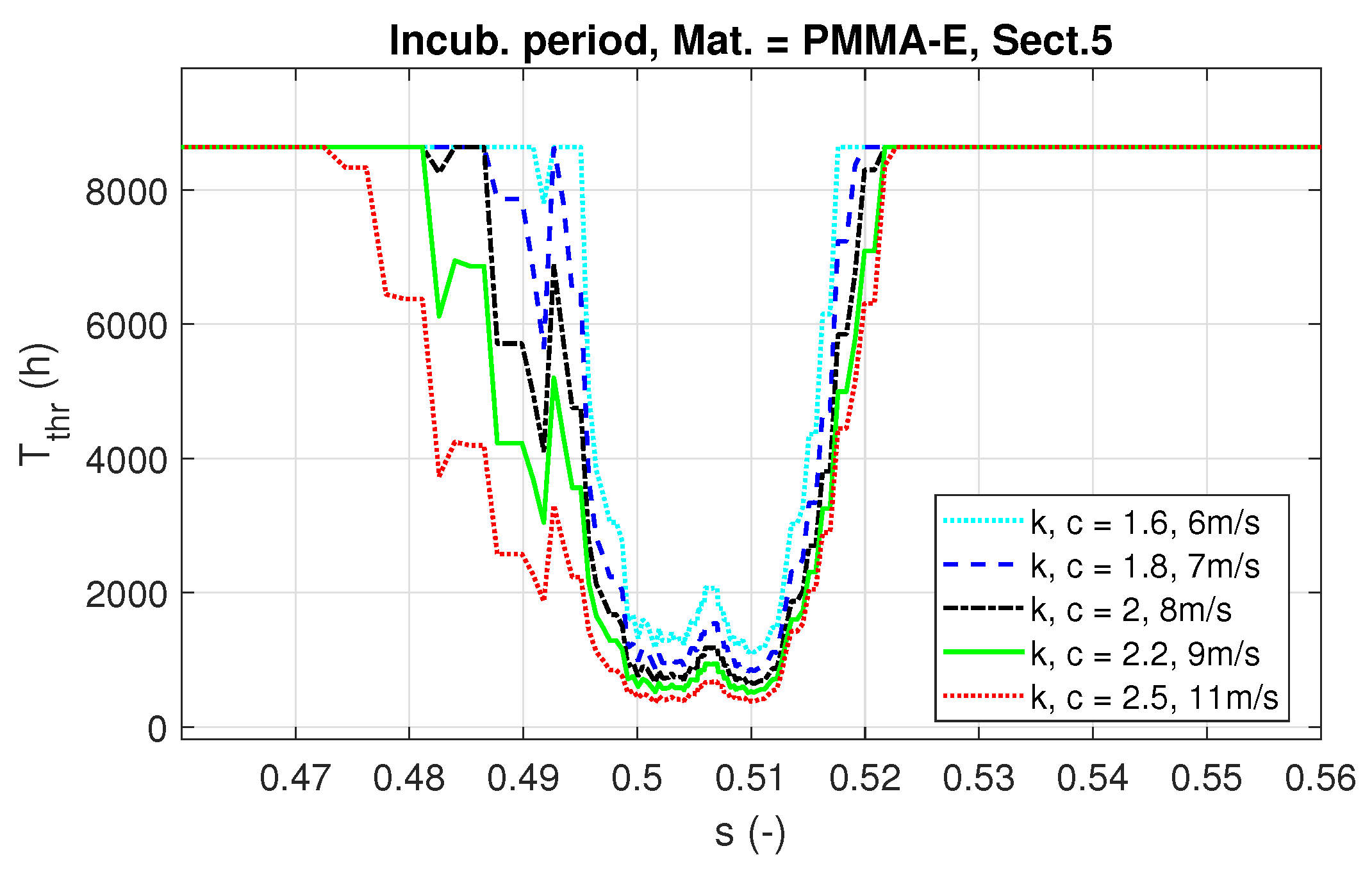
3.1. Erosion Damage Incubation Maps

Figure 5 reports a view of the variation of the damage fraction n p / ( n p ) t h r per hour along the airfoil coordinate s.
It is immediately evident from Figure 5a that, according to this model, the material that offers the lowest resistance to erosion is PMMA-E, which is then taken as the reference for the other analyses of the fixed material. Figure 5b shows that erosion would start from section 5 (containing the maximum value), which is located at 93.33% of the blade span and has a chord of 2.09 m. This result was expected as section 5 has the second highest relative velocity in the set of the selected section, but section 6 (the section at the blade tip) has half of the chord length; therefore, it offers half of the surface to the rain flow, reducing the number of possible impacts with respect to section 5. This result is in line with a former 3D analysis of rain erosion damage made by the authors [23].
Fixing the section and material to the worst case in terms of erosion resistance, it is possible to continue the discussion investigating the influence of mean wind velocity (the wind turbine working condition) and rain flow rate on the distribution of the variables n p / ( n p ) t h r over the airfoil shape (Figure 5c and Figure 6, respectively). Figure 5c shows an obvious result as the damage fraction n p / ( n p ) t h r (the inverse of the incubation period) increases with the rain flow rate, because a higher rain flow rate means a higher droplet concentration. However, the scale up is not linear because higher flow rates correspond to different droplet size distributions which in turn affect the particle dynamics. A much more interesting view is given by Figure 6 which shows how the area mostly affected by the damage changes, passing from a higher effect on the pressure side for the operating condition at a wind speed lower than the rated one (around 11 m/s) to a higher effect on the suction side for operation at a wind stronger than the rated speed. This is due to the pitch control system, which reduces the angle of attack of the blade section down to negative values in pitch-controlled operations, thus exposing a larger portion of the suction side to droplet impacts. It is also important to note that the region affected by a value of n p / ( n p ) t h r > 0.001 ( T t h r < 1000 h), in all cases, extends from the leading edge (LE) for no more than 2% on the pressure side and 3% on the suction side. Outside this region, the aforementioned ratio drops to negligibly small values. This result is an effect of the airfoil shape, and similar extensions of the erosion pattern have been computed in previous works [24,25,26] and observed in the field [44].
Figure 7 shows the curves of the minimum incubation period predicted at each average wind velocity V for PMMA-E applied to section 5 at different rain flow rates. As expected, the main trend of the envelopes follows the variation of the rotor angular velocity, which increases from the cut-in to the rated wind speed (4 to 11 m/s), and then it is kept fixed to the maximum value for wind speeds above the rated value. The absolute minimum of the incubation period is expected, according to this model, close to the rated wind speed (at V = 13 m/s). For wind speeds larger than 13 m/s, the model predicts a general increase in the incubation period. We can explain this behavior by noticing that in the wind time series generated for this study, turbulent fluctuations of the velocity increase with an increasing mean wind speed. Larger amplitude fluctuations of the velocity result in an enlargement of the main particle-impacting region, which results in a lower peak of impacts per unit surface at the end of the 10 min record. A further investigation will be needed in the future to establish the model uncertainties associated with neglecting the dynamic effects in the particle flow interacting with a fluctuating wind.

3.2. Application for a Specific Installation Site

The results of the computations based on Equation (9), for the various blade sections and materials, are shown in Table 4. As expected from the analyses of the damage incubation maps ( n i / ( n p ) t h r ) in Section 3.1, the material offering the lowest resistance is PMMA-E. In this case, when a blade covered by this material is working for one year at the rain and wind of Figure 4, the model predicts that erosion starts at section 5 after 445 h of operation. With 8640 h in a year, we can verify from Table 4 the regions where erosion is expected after a year of operation. For example, erosion will also start in the regions of sections 5 and 6 for a blade covered by the other tested material (PMMA-C).
Figure 8 shows a 3D plot of the incubation period computed in the range of blade span r covered by the six sections of Figure 3 and for s ranging between 47 and 53% of the section curvilinear length. It can be noted how the shape of the plot does not qualitatively change among different sections; however, the minimum incubation time occurs at the fifth section (93.33% of the span) as was already noted for the analyses reported in Section 3.1.
An interesting analysis is provided in Figure 9, where the same computation has been repeated for different wind annual statistics. In particular, for sites featuring stronger winds (higher k and c factors), there is a small reduction in the incubation time and an enlargement of the area possibly affected by erosion toward the suction side. The reason is rooted in the same considerations made by reference to Figure 6; these sites are characterized by a higher probability to encounter winds stronger than the rated wind speed defined by the turbine design. Therefore, the pitch control would act more often, exposing the suction side to the erosion of the rain droplets.

4. Conclusions

The paper has two main objectives, which are to present a methodology for estimating the resistance of a wind blade surface to rain erosion and to report a practical example of applying this methodology to a specific case of installation in a rainy environment.
The methodology is based on the integration of CFD, particle tracking, machine learning, a rain erosion model, with the statistical description of rain and wind at a given site, and with the multibody simulation of the turbine using openfast.
The final estimation of the damage incubation period over a set of radial sections of the blade has been computed, starting from the definition of a set of damage incubation maps per hour of exposition of each section to a matrix of rain flows and wind velocities. The maps have been generated using an impact pattern prediction system which can account for airfoil geometry, the local variation of aerodynamics and particle flow due to wind turbulence and wind turbine control.
Thanks to the system presented, it has been possible to evaluate the region and extension over the blade surface possibly affected by erosion damage already after a year of operation for two possible versions of PMMA coating material. The results are in agreement with field observations in terms of the distribution of the damage area over the blade surface and the identification of the most sensible regions, providing also a reasonable incubation time for a blade operating in the environment assumed for the numerical testing.
We notice that, although it is possible to verify the accuracy of the single modules and methods integrated in the final prediction system, the quantification of the uncertainty associated to the final numeric result is an open challenge, which requires the comparison with field measurements that are not available nowadays in a form suitable for a rigorous validation.

Author Contributions

A.C. and P.V.: conceptualization; methodology; software; validation; investigation; resources; data curation; writing—original draft preparation; writing—review and editing; visualization; supervision; project administration; funding acquisition; formal analysis. A.B.: supervision; writing—review and editing. All authors have read and agreed to the published version of the manuscript.

Funding

This research received no external funding.

Institutional Review Board Statement

Not applicable.

Informed Consent Statement

Not applicable.

Data Availability Statement

Not applicable.

Conflicts of Interest

The authors declare no conflict of interest. The funders had no role in the design of the study; in the collection, analyses, or interpretation of data; in the writing of the manuscript; or in the decision to publish the results.

References

  1. United Nations. Glasgow Climate Pact. In Proceedings of the Conference of the Parties Serving as the Meeting of the Parties to the Paris Agreement, Glasgow, UK, 31 October–12 November 2021. [Google Scholar]
  2. United Nations. Paris Agreement. In Proceedings of the Paris Climate Change Conference (COP21), Paris, France, 30 November–12 December 2015. [Google Scholar]
  3. IRENA. World Energy Transitions Outlook 2022: 1.5 °C Pathway; International Energy Renewable Agency: Abu Dhabi, United Arab Emirates, 2022. [Google Scholar]
  4. WWEA. Global Wind Installation. Technical Report. Available online: https://library.wwindea.org/global-statistics/ (accessed on 31 May 2022).
  5. IRENA. Future of Wind, Deployment, Investment, Technology, Grid Integration and Socio-Economic Aspects (A Global Energy Transformation Paper); Technical Report; International Renewable Energy Agency: Abu Dhabi, United Arab Emirates, 2019. [Google Scholar]
  6. Oettinger, G.H. Energy, Roadmap 2050; Technical Report; European Commission: Luxembourg, 2011.
  7. Enevoldsen, P.; Xydis, G. Examining the trends of 35 years growth of key wind turbine components. Energy Sustain. Dev. 2019, 50, 18–26. [Google Scholar] [CrossRef]
  8. Igwemezie, V.; Mehmanparast, A.; Kolios, A. Current trend in offshore wind energy sector and material requirements for fatigue resistance improvement in large wind turbine support structures—A review. Renew. Sustain. Energy Rev. 2019, 101, 181–196. [Google Scholar] [CrossRef] [Green Version]
  9. Cappugi, L.; Castorrini, A.; Bonfiglioli, A.; Minisci, E.; Campobasso, M.S. Machine learning-enabled prediction of wind turbine energy yield losses due to general blade leading edge erosion. Energy Convers. Manag. 2021, 245, 114567. [Google Scholar] [CrossRef]
  10. Dalili, N.; Edrisy, A.; Carriveau, R. A review of surface engineering issues critical to wind turbine performance. Renew. Sustain. Energy Rev. 2009, 13, 428–438. [Google Scholar] [CrossRef]
  11. Rempel, L. Rotor blade leading edge erosion-real life experiences. Wind. Syst. Mag. 2012, 11, 22–24. [Google Scholar]
  12. Mishnaevsky, L., Jr. Toolbox for optimizing anti-erosion protective coatings of wind turbine blades: Overview of mechanisms and technical solutions. Wind Energy 2019, 22, 1636–1653. [Google Scholar] [CrossRef]
  13. Verma, A.S.; Noi, S.D.; Ren, Z.; Jiang, Z.; Teuwen, J.J.E. Minimum Leading Edge Protection Application Length to Combat Rain-Induced Erosion of Wind Turbine Blades. Energies 2021, 14, 1629. [Google Scholar] [CrossRef]
  14. Herring, R.; Dyer, K.; Martin, F.; Ward, C. The increasing importance of leading edge erosion and a review of existing protection solutions. Renew. Sustain. Energy Rev. 2019, 115, 109382. [Google Scholar] [CrossRef]
  15. Bech, J.I.; Hasager, C.B.; Bak, C. Extending the life of wind turbine blade leading edges by reducing the tip speed during extreme precipitation events. Wind. Energy Sci. 2018, 3, 729–748. [Google Scholar] [CrossRef] [Green Version]
  16. Hu, W.; Chen, W.; Wang, X.; Jiang, Z.; Wang, Y.; Verma, A.S.; Teuwen, J.J. A computational framework for coating fatigue analysis of wind turbine blades due to rain erosion. Renew. Energy 2021, 170, 236–250. [Google Scholar] [CrossRef]
  17. Li, D.; Zhao, Z.; Li, Y.; Wang, Q.; Li, R.; Li, Y. Effects of the particle Stokes number on wind turbine airfoil erosion. Appl. Math. Mech. 2018, 39, 639–652. [Google Scholar] [CrossRef]
  18. O’Carroll, A.; Hardiman, M.; Tobin, E.; Young, T. Correlation of the rain erosion performance of polymers to mechanical and surface properties measured using nanoindentation. Wear 2018, 412–413, 38–48. [Google Scholar] [CrossRef]
  19. Springer, G.S.; Yang, C.I.; Larsen, P.S. Analysis of rain erosion of coated materials. J. Compos. Mater. 1974, 8, 229–252. [Google Scholar] [CrossRef]
  20. Miner, M.A. Cumulative damage in fatigue 1945. J. Appl. Mech. 1945, 12, A159–A164. [Google Scholar] [CrossRef]
  21. Elhadi Ibrahim, M.; Medraj, M. Water droplet erosion of wind turbine blades: Mechanics, testing, modeling and future perspectives. Materials 2019, 13, 157. [Google Scholar] [CrossRef] [Green Version]
  22. Corsini, A.; Castorrini, A.; Morei, E.; Rispoli, F.; Sciulli, F.; Venturini, P. Modeling of rain drop erosion in a multi-MW wind turbine. In Proceedings of the ASME Turbo Expo 2015: Turbine Technical Conference and Exposition. Volume 9: Oil and Gas Applications; Supercritical CO2 Power Cycles; Wind Energy, Montreal, QC, Canada, 15–19 June 2015. [Google Scholar] [CrossRef]
  23. Castorrini, A.; Corsini, A.; Rispoli, F.; Venturini, P.; Takizawa, K.; Tezduyar, T.E. Computational analysis of wind-turbine blade rain erosion. Comput. Fluids 2016, 141, 175–183. [Google Scholar] [CrossRef]
  24. Castorrini, A.; Corsini, A.; Rispoli, F.; Venturini, P.; Takizawa, K.; Tezduyar, T.E. Computational analysis of performance deterioration of a wind turbine blade strip subjected to environmental erosion. Comput. Mech. 2019, 64, 1133–1153. [Google Scholar] [CrossRef]
  25. Castorrini, A.; Venturini, P.; Gerboni, F.; Corsini, A.; Rispoli, F. Machine Learning Aided Prediction of Rain Erosion Damage on Wind Turbine Blade Sections. In Proceedings of the ASME Turbo Expo 2021: Turbomachinery Technical Conference and Exposition, Volume 1: Aircraft Engine, Fans and Blowers, Marine, Wind Energy, Scholar Lecture, Virtual, 7–11 June 2021; p. V001T40A002. [Google Scholar] [CrossRef]
  26. Castorrini, A.; Venturini, P.; Corsini, A.; Rispoli, F. Machine learnt prediction method for rain erosion damage on wind turbine blades. Wind Energy 2021, 24, 917–934. [Google Scholar] [CrossRef]
  27. Jonkman, J.; Sprague, M. Openfast: An Aeroelastic Computer-Aided Engineering Tool for Horizontal Axis Wind Turbines; National Renewable Energy Laboratory: Golden, CO, USA, 2020; Volume 17.
  28. Jonkman, B.J. TurbSim User’s Guide: Version 1.50; Technical Report; National Renewable Energy Lab. (NREL): Golden, CO, USA, 2009.
  29. Serio, M.A.; Carollo, F.G.; Ferro, V. Raindrop size distribution and terminal velocity for rainfall erosivity studies. A review. J. Hydrol. 2019, 576, 210–228. [Google Scholar] [CrossRef]
  30. Blocken, B.; Carmeliet, J. Driving rain on building envelopes-I. Numerical estimation and full-scale experimental verification. J. Therm. Envel. Build. Sci. 2000, 24, 61–85. [Google Scholar]
  31. Best, A. The size distribution of raindrops. Q. J. R. Meteorol. Soc. 1950, 76, 16–36. [Google Scholar] [CrossRef]
  32. Pruppacher, H.R.; Pitter, R. A semi-empirical determination of the shape of cloud and rain drops. J. Atmos. Sci. 1971, 28, 86–94. [Google Scholar] [CrossRef] [Green Version]
  33. CROW. Typical Poisson’s Ratios of Polymers at Room Temperature. Available online: https://polymerdatabase.com (accessed on 28 April 2022).
  34. SONELASTIC—Division of ATCP Physical Engineering. Modulus of Elasticity and Poisson’s Coefficient of Polymeric Materials. Available online: https://www.sonelastic.com/en/fundamentals/tables-of-materials-properties/polymers.html (accessed on 28 April 2022).
  35. Amesweb—Advanced Mechanical Engineering Solutions. Poisson’s Ratio of Polymers. Available online: https://amesweb.info/Materials/Poissons_Ratio_of_Polymers.aspx (accessed on 28 April 2022).
  36. Phoenix Technologies International L.L.C. Polyethylene Terephtalate Key Properties. Available online: phoenixtechnologies.net (accessed on 28 April 2022).
  37. INEOS Olefins and Polymers USA. Typical Engineering Properties of Polypropylene. Available online: phoenixtechnologies.net (accessed on 28 April 2022).
  38. Professional Plastic Inc. Mechanical Properties of Plastic Materials. Available online: https://www.professionalplastics.com/professionalplastics/MechanicalPropertiesofPlastics.pdf (accessed on 28 April 2022).
  39. Vinidex, by Aliaxis. Material Properties. Available online: https://www.vinidex.com.au/technical-resources/material-properties/ (accessed on 28 April 2022).
  40. Li, T.C.; Han, C.F.; Chen, K.T.; Lin, J.F. Fatigue Life Study of ITO/PET Specimens in Termsof Electrical Resistance and Stress/Strain via Cyclic Bending Tests. J. Disp. Technol. 2013, 9, 577–585. [Google Scholar] [CrossRef]
  41. Mott, P.; Dorgan, J.; Roland, C. The bulk modulus and Poisson’s ratio of “incompressible” materials. J. Sound Vib. 2008, 312, 572–575. [Google Scholar] [CrossRef]
  42. Jonkman, J.; Butterfield, S.; Musial, W.; Scott, G. Definition of a 5-MW Reference wind Turbine for Offshore System Development; Technical Report; National Renewable Energy Lab. (NREL): Golden, CO, USA, 2009.
  43. Verma, A.S.; Jiang, Z.; Caboni, M.; Verhoef, H.; van der Mijle Meijer, H.; Castro, S.G.; Teuwen, J.J. A probabilistic rainfall model to estimate the leading-edge lifetime of wind turbine blade coating system. Renew. Energy 2021, 178, 1435–1455. [Google Scholar] [CrossRef]
  44. Sareen, A.; Sapre, C.A.; Selig, M.S. Effects of leading edge erosion on wind turbine blade performance. Wind Energy 2014, 17, 1531–1542. [Google Scholar] [CrossRef]
Figure 1. Definition of airfoil curvilinear coordinate s.
Energies 15 05593 g001
Figure 2. Probability density function of the raindrop sizes varying R h .
Energies 15 05593 g002
Figure 3. Blade surface, target areas and sections.
Energies 15 05593 g003
Figure 4. Probability density functions for hourly rain intensity (top) and wind velocity (bottom).
Energies 15 05593 g004
Figure 5. Erosion damage maps varying blade material (a), blade section (b) and rain intensity (c).
Energies 15 05593 g005
Figure 6. Erosion damage map at different wind velocities.
Energies 15 05593 g006
Figure 7. Minimum incubation period for section 5 and PMMA-E test case.
Energies 15 05593 g007
Figure 8. Incubation period over the blade surface for the PMMA-E coating material, having considered a one-year operation with rain and wind statistics of Figure 4.
Energies 15 05593 g008
Figure 9. Incubation period at section 5 for the PMMA-E coating material, having considered one-year operation with rain statistics of Figure 4 and varying the scale (c) and shape (k) parameters of the Weibull wind speed distribution.
Energies 15 05593 g009
Table 1. Main characteristics of the materials tested in [18].
PropertyPMMA-CPMMA-E
Density (kg/m 3 )1222.71212.6
Elastic modulus (GPa)5.104.28
Poisson’s ratio * (-)0.33–0.410.33–0.41
Ultimate tensile strength (MPa)78.070.5
Speed of sound (m/s)27742727
* Sources: [33,34,35,36,37,38,39,40,41].
Table 2. Experimental incubation period and corresponding Poisson’s ratio and a 2 values obtained for the materials tested in [18].
ValuePMMA-CPMMA-E
Incubation period (min)164
Poisson’s ratio (-)0.410.36
a 2 5.6835.668
Table 3. NREL 5MW blade sections and identification of the section IDs for the erosion analysis.
Blade Span (%)Twist (∘)Chord (m)AirfoilSect. ID
0.0013.313.54cylinder-
2.2213.313.54cylinder-
6.6713.313.85cylinder-
11.1113.314.17cylinder-
16.6713.314.56DU99W405-
23.3311.484.65DU99W350-
30.0010.164.46DU99W350-
36.679.014.25DU97W300-
43.337.804.01DU91W250-
50.006.543.75DU91W250-
56.675.363.50DU93W210-
63.334.193.26DU93W210-
70.003.133.01NACA646181
76.672.322.76NACA646182
83.331.532.52NACA646183
88.890.862.31NACA646184
93.330.372.09NACA646185
97.780.111.42NACA646186
100.000.111.42NACA64618-
Table 4. Incubation period (in hours) matrix per section and material.
MaterialSection 1Section 2Section 3Section 4Section 5Section 6
PMMA-C21,180 h14,523 h10,757 h8545 h7598 h12,214 h
PMMA-E1233 h847 h628 h499 h445 h715 h
Publisher’s Note: MDPI stays neutral with regard to jurisdictional claims in published maps and institutional affiliations.

