Velocity Sensor Fault-Tolerant Controller for Induction Machine Using Intelligent Voting Algorithm

Abstract

Nowadays, induction machines (IMs) are widely used in industrial and transportation applications (electric or hybrid ground vehicle or aerospace actuators) thanks to their significant advantages in comparison to other technologies. Indeed, there is a large demand for IMs because of their reliability, robustness, and cost-effectiveness. The objective of this paper is to improve the reliability and performance of the three-phase induction machine in case of mechanical sensor failure. Moreover, this paper will discuss the development and proposal of a fault-tolerant controller (FTC), based on the combination of a vector controller, two virtual sensors (an extended Kalman filter, or EKF, and a sliding mode observer, or SMO) and a neural voting algorithm. In this approach, the vector controller is based on a new structure of a back-stepping sliding mode controller, which incorporates a double integral sliding surface to improve the performance of the induction machine in faulty operation mode. More specifically, this controller improves the machine performance in terms of having a fast response, fewer steady-state errors, and a robust performance in the existence of uncertainty. In addition, two voting algorithms are suggested in this approach. The first is based on neural networks, which are insensitive to parameter variations and do not need to set a threshold. The second one is based on fuzzy logic. Finally, validation is carried out by simulations in healthy and faulty operation modes to prove the feasibility of the proposed FTC.

1. Introduction

In today’s industry, the main requirements for any system are performance, efficiency, availability, reliability, and safety, in addition to productivity. Therefore, monitoring and supervisory functions are highly prioritized in the control unit of any system to achieve these goals. These functions consist of developing methods of detection, isolating faults, and using fault-tolerant control to maintain good performance in faulty operation mode. Indeed, fault tolerance has become an increasingly more interesting topic in the last decade for modern technological and safety-critical systems [1,2]. In fact, FTC is of utmost importance for every aspect of safety-critical systems such as in airplanes and nuclear reactors. It specifically hinders faults from growing into full failures [3]. These failures may have life-threatening impacts on humans. Human history has witnessed several accidents which can be avoided if control systems are designed to be tolerant of faults. Examples of these accidents include the disaster at the Chernobyl nuclear power plant in 1986 and the Three Mile Island accident in 1979. Therefore, interest in FTC systems has increased since the 1980s [4]. For more information about the last applications of FTC, one can look at [5,6] and the references therein.

Due to its low cost, structural robustness, and high efficiency, the induction machine (IM) is becoming competitive in many applications, such as railway electric propulsion power trains, wind turbines, etc. [7,8]. Unfortunately, this machine can be affected by different faults, which may yield drastic consequences. The main faults which can occur in the induction machine drive are stator faults (open phase, short-circuit, electrical discharges, etc.) [9,10], inverter faults (short-circuit and open-circuit) [11,12], and sensor faults [1,13,14].

However, a mechanical sensor failure can lead to instability and a decline in performance [1,14]. Consequently, the fault diagnosis of the speed sensor will ensure reliability and continuity of operation in the industrial sector with a minimum level of performance in case of speed sensor failure. Therefore, the diagnosis of mechanical sensor failure has received considerable attention in the literature [1,7,13,14,15,16].

For IM speed sensor failure, two approaches have been developed in the literature. In the first approach, when a faulty speed sensor is detected, the control algorithm is reconfigured using a new control law [7,15]. In the second approach, when a speed sensor fault is detected, an observer is used instead of the speed sensor in the control loop. Usually, one or two observers are employed. In the case of a single observer, the residuals obtained by calculating the difference between measured and estimated speeds are used, and these are compared to a predefined threshold for detecting faulty operation modes. Unfortunately, the computed residual value diverges from zero even in the healthy operation mode. This is due to model uncertainties and parameter variations, which complicate the selection of an appropriate threshold value [17]. In the case of two observers, a voting algorithm is used to compute the most accurate information related to speed from the sensor and the observers [1].

Several voting techniques have been described in the literature, and these have been widely used in safety-critical applications and FTC systems, such as weighted average voters (WAV) [18], the fuzzy voter (FV) [19], the maximum-likelihood voter (MLV) [1,20], the Euler voter (EV) [21], and the Newton-Raphson voter (NRV) [21]. A major difficulty with these voters is the need to choose an appropriate threshold value, which has a direct impact on voter performance, especially in the presence of parameter variations.

The WAVs suffer from a lack of accuracy in normal conditions, i.e., without a fault, because the measured speed is mixed with the estimated ones, which then leads to less accurate values [1]. Moreover, the faulty sensor still contributes to the final output of the voter even with a small weight in the faulty case. The MLV chooses the sensor or the observer that has the maximum likelihood without mixing between the estimated and the measured speeds [1]. However, the quality of MLV depends on the correct setting of its threshold, which has a direct impact on the voter performance, especially in the presence of parameter variations. The EV produces an estimated signal based on the Euler approximation of the real measured signal. Then, the estimated signal must be compared with the voter inputs to achieve the voting process [21]. Nevertheless, EV is sensitive to the rapid changes of the real signal, which reduces the estimation accuracy. In NRV, a numerical threshold value must be set which directly affects the voter performance [21].

In this paper, an IM speed sensor FTC is proposed. It is based on the combination of the actual sensor and two virtual ones, namely an extended Kalman filter (EKF) and a sliding mode observer (SMO). A new voting algorithm based on neural networks is suggested to solve the problem of choosing an appropriate threshold value. The proposed algorithm is compared to a fuzzy voter that is modified and adapted for the task of sensor fault-tolerant control. In addition, to ensure response speed with high performance, a controller is created by connecting an integral back-stepping controller with a double integral sliding mode controller. The suggested integral back-stepping double integral sliding mode (IBS-DISMC) controller aims to further improve performance in terms of having a fast response, fewer steady-state errors, and a robust performance in the existence of uncertainty. The novelty of this work can be summarized using the following points:

• The new proposed controller (IBS-DISMC) is introduced to improve the performance of the IM under faulty conditions. Specifically speaking, IBS-DISMC has a fast response, fewer steady-state errors, and a robust performance in the existence of uncertainty.
• The new neural voting algorithm is proposed to avoid setting up a threshold, which is the main limitation of the reported voting algorithms in the literature. Additionally, the proposed voter has a good robustness against parameter variations.
• The fuzzy voter given in [19] is modified to be applicable for diagnosing the failure of a velocity sensor of an induction machine.

In this paper, Section 2 is devoted to the proposed controller and its validation by simulation. Section 3 presents the mathematical models of the extended Kalman filter and the sliding mode observers, in order to estimate the induction machine speed and their validation by simulation to evaluate their performance. Section 4 is devoted to the developed approach of FTC, the proposed voting algorithms, and their validation by simulation in a faulty operation mode, showing the benefit of the suggested method to isolate, with a high reliability, the speed sensor fault. Finally, in Section 5, conclusions about the carried-out work are presented.

2. Controller Design

As parameter variations severely affect the performance of the voting algorithm, a robust control algorithm is required to reduce the effects of parameter changes. Back-stepping control (BSC) [22] and sliding mode control (SMC) [23] are suggested as powerful control algorithms in many applications. The BSC technique has frequently been used for controlling nonlinear systems. However, the BS controller cannot handle uncertainty quickly. Therefore, connecting the BSC with the SMC can help to overcome this weakness and provide a more robust controller [24]. Additionally, this hybrid structure reduces the adverse effects of chattering of SMC and applies less control effort compared with SMC [25]. Double integral sliding mode control (DISMC) is another recent approach for dealing with nonlinear systems. According to the mathematical theory, DISMC basically constructs the sliding surface using double integral terms [26]. DISMC is used to eliminate the steady-state errors [26], and to provide a fast response with better performance for system uncertainty [27]. Here, for improving the performance of IM vector control (fast response, fewer steady-state errors, and robust performance in the existence of uncertainty), a new control scheme is suggested. Figure 1 shows the architecture of the designed controller using the integral back-stepping of Jia et al. [24], and the double integrator sliding mode controller of Qureshi et al. [26].

2.1. Presentation of the Analytical d-q Model of the Induction Machine

The mathematical model of IM in the (d, q) frame [28] is given by the following:

$$\frac{d{i}_{sd}}{dt}=\alpha i_{sd}+\beta {\psi }_d+p\Omega i_{sq}+\begin{array}{c}\gamma \end{array}{i}^2{}_{sq}/{\psi }_d+a{u}_{sd}$$

(1)

$$\frac{d{i}_{sq}}{dt}=\alpha i_{sq}-cp\Omega {\psi }_d-p\Omega i_{sd}-\begin{array}{c}\gamma \end{array}{i}_{sq}{i}_{sd}/{\psi }_d+a{u}_{sq}$$

(2)

$$\frac{d{\psi }_d}{dt}=\delta {\psi }_d+\begin{array}{c}\gamma \end{array}{i}_{sd}$$

(3)

$$J\frac{d\Omega }{dt}=T_e-T_L$$

(4)

$$T_e=J\vartheta {\psi }_d{i}_{sq}$$

(5)

where u_sd and $u_{sq}$ are the stator voltages. $i_{sd}$ and $i_{sq}$ denote the stator currents. ${\psi }_d$ represents the rotor flux. $\Omega$ stands for the motor mechanical speed. $T_L$ and $T_e$ are the load and electromagnetic torques. The parameters of Equations (1)–(5) are given as follows:

$$\begin{gathered} \sigma =1-\frac{L^2{}_{sr}}{L_s{L}_r},\alpha =-\left(a{R}_s+c\frac{L_{sr}}{T_r}\right),a=\frac{1}{\sigma L_s},c=\frac{1-\sigma }{\sigma L_{sr}}, \\ {T}_r=\frac{L_r}{R_r},\beta =\frac{c}{T_r},\gamma =\frac{L_{sr}}{T_r},\delta =\frac{-1}{T_r},\vartheta =\frac{p{L}_{sr}}{J{L}_r} \end{gathered}$$

$R_s$ and $R_r$ are stator and rotor resistances. $L_s$, $L_r$, and $L_{sr}$ are, respectively, stator, rotor and mutual inductances. $p$ is the number of pole pairs and $J$ is the moment of inertia.

2.2. Suggestion

Based on the (d, q) model of the IM, an integral back-stepping double integrator sliding mode controller (IBS-DISMC) is designed. The next subsection will be devoted to explaining the proposed controller.

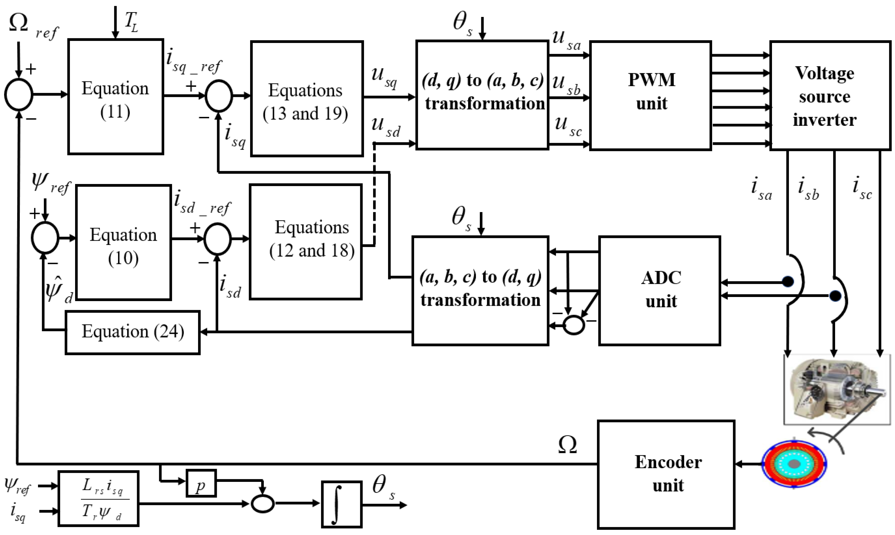
2.3. Integral Back-Stepping Double Integrator Sliding Mode Controller

IBS-DISMC uses the following tracking errors of rotor flux and speed:

$$e_1={\psi }_{d\_ref}-{\psi }_d+\int \left({\psi }_{d\_ref}-{\psi }_d\right)dt$$

(6)

$$e_2={\Omega }_{d\_ref}-{\Omega }_d+\int \left({\Omega }_{d\_ref}-{\Omega }_d\right)dt$$

(7)

Here, ${\psi }_{d\_ref}$ and ${\Omega }_{d\_ref}$ are, respectively, the desired values of rotor flux and speed. The time derivative of (6) and (7) can be calculated as follows:

$${\dot{e}}_1={\dot{\psi }}_{d\_ref}-\delta {\psi }_d-\begin{array}{c}\gamma \end{array}{i}_{sd}+{\psi }_{d\_ref}-{\psi }_d$$

(8)

$${\dot{e}}_2={\dot{\Omega }}_{d\_ref}-\vartheta {\psi }_d{i}_{sq}+\frac{T_L}{J}+{\Omega }_{d\_ref}-{\Omega }_d$$

(9)

Considering the Lyapunov function $V_1=0.5e_1^2+0.5e_2^2$, and its derivative ${\dot{V}}_1=e_1{\dot{e}}_1+e_2{\dot{e}}_2$, ${\dot{e}}_1$ and ${\dot{e}}_2$ can be computed as follows:

$${\dot{e}}_1=-k_1{e}_1\mathrm{and}{\dot{e}}_2=-k_2{e}_2$$

to guarantee the system stability, i.e., ${\dot{V}}_1<0$. Here, $k_1$ and $k_2$ are positive constants.

Considering the above discussion, the following control laws can be obtained:

$$i_{sd}{}_{\_ref}=\frac{1}{\gamma }\left(k_1{e}_1+{\dot{\psi }}_{d\_ref}-\left(1+\delta \right){\psi }_d+{\psi }_{d\_ref}\right)$$

(10)

$$i_{sq\_ref}=\frac{1}{\vartheta {\psi }_d}\left(k_2{e}_2+{\dot{\Omega }}_{ref}+\frac{T_L}{J}+{\Omega }_{ref}-\Omega \right).$$

(11)

To design the reference voltages, the following double integral sliding surfaces are considered:

$$s_1=\left(i_{sd\_ref}-i_{sd}\right)+k_3\int \left(i_{sd\_ref}-i_{sd}\right)dt+k_4\int \left\{\int \left(i_{sd\_ref}-i_{sd}\right)dt\right\}dt$$

(12)

$$s_2=\left(i_{sq\_ref}-i_{sq}\right)+k_5\int \left(i_{sq\_ref}-i_{sq}\right)dt+k_6\int \left\{\int \left(i_{sq\_ref}-i_{sq}\right)dt\right\}dt$$

(13)

Here, $k_3$, $k_4$, $k_5$, and $k_6$ are positive constants. The derivative of the above sliding surfaces can be expressed as follows:

$${\dot{s}}_1=\frac{d{i}_{sd\_ref}}{dt}-f_d-a{u}_{sd}+k_3\left(i_{sd\_ref}-i_{sd}\right)+k_4\int \left(i_{sd\_ref}-i_{sd}\right)dt$$

(14)

$${\dot{s}}_2=\frac{d{i}_{sq\_ref}}{dt}-f_q-a{u}_{sq}+k_5\left(i_{sq\_ref}-i_{sq}\right)+k_6\int \left(i_{sq\_ref}-i_{sq}\right)dt$$

(15)

where:

• $f_d=\alpha i_{sd}+\beta {\psi }_d+p\Omega i_{sq}+\begin{array}{c}\gamma \end{array}{i}^2{}_{sq}/\psi$ and $f_q=\alpha i_{sq}-cp\Omega {\psi }_d-p\Omega i_{sd}-\begin{array}{c}\gamma \end{array}{i}_{sq}{i}_{sd}/{\psi }_d$.

After solving the sliding mode condition ${\dot{s}}_1=0$ and ${\dot{s}}_2=0$ for input signals $u_{sd}$ and $u_{sq}$, the equivalent control laws $u_{sd\_eq}$ and $u_{sq\_eq}$ can described as follows:

$$u_{sd\_eq}=\frac{1}{a}(\frac{d{i}_{sd\_ref}}{dt}-f_d+k_3\left(i_{sd\_ref}-i_{sd}\right)+k_4\int \left(i_{sd\_ref}-i_{sd}\right)dt)$$

(16)

$$u_{sq\_eq}=\frac{1}{a}(\frac{d{i}_{sq\_ref}}{dt}-f_q+k_5\left(i_{sq\_ref}-i_{sq}\right)+k_6\int \left(i_{sq\_ref}-i_{sq}\right)dt)$$

(17)

The mathematical forms of the discontinuous control laws are defined as follows:

$$\Delta u_1=k_{s_1}\mathit{sgn}(s_1)\mathrm{and}\Delta u_2=k_{s_2}\mathit{sgn}(s_2)$$

In addition, using Equations (16) and (17), we can finally deduce the control laws $u_{sd}$ and $u_{sq}$ of IBS-DISMC as follows:

$$u_{sd}=u_{sd\_eq}+\Delta u_1\mathrm{and}{u}_{sq}=u_{sq\_eq}+\Delta u_2$$

$$u_{sd}=[\frac{1}{a}(\frac{d{i}_{sd\_ref}}{dt}-f_d+k_3\left(i_{sd\_ref}-i_{sd}\right)+k_4\int \left(i_{sd\_ref}-i_{sd}\right)dt)]+k_{s_1}\mathit{sgn}(s_1)$$

(18)

$$u_{sq}=[\frac{1}{a}(\frac{d{i}_{sq\_ref}}{dt}-f_q+k_5\left(i_{sq\_ref}-i_{sq}\right)+k_6\int \left(i_{sq\_ref}-i_{sq}\right)dt)]+k_{s_2}\mathit{sgn}(s_2)$$

(19)

To check the stability of the suggested controller, the following Lyapunov positive function is defined as follows:

$$V=0.5e_1{}^2+0.5e_2{}^2+0.5s_1{}^2+0.5s_2{}^2$$

(20)

Its derivative is given by the following:

$$\dot{V}=e_1{\dot{e}}_1+e_2{\dot{e}}_2+s_1{\dot{s}}_1+s_2{\dot{s}}_2.$$

(21)

From the conditions in which the integral back-stepping control laws were established i.e., ${\dot{e}}_1=-k_1{e}_1$ and ${\dot{e}}_2=-k_2{e}_2$, and using (14) and (15), Equation (21) becomes as follows:

$$\begin{array}{cc}\hfill \dot{V}=-k_1{e}_1{}^2+k_2{e}_2{}^2& +s_1(\frac{d{i}_{s{d}_{ref}}}{dt}-f_d-a{u}_{sd}+k_3\left(i_{s{d}_{ref}}-i_{sd}\right)+k_4\int \left(i_{sd\_ref}-i_{sd}\right)dt)\hfill \\ & +s_2(\frac{d{i}_{sq\_ref}}{dt}-f_q-a{u}_{sq}+k_5\left(i_{sq\_ref}-i_{sq}\right)+k_6\int \left(i_{sq\_ref}-i_{sq}\right)dt)\hfill \end{array}$$

(22)

Compensating the control laws $u_{sd}$ and $u_{sq}$, given in (16) and (17), into (22), the derivative of Lyapunov function can be reformulated as follows:

$$\dot{V}=-k_1{e}_1{}^2+k_2{e}_2{}^2-a{k}_{s_1}\left|s_1\right|-a{k}_{s_2}\left|s_2\right|$$

(23)

where $k_1$, $k_2$, $a$, $k_{s_2}$, and $k_{s_1}$ are positive constants. Therefore, the derivative of Lyapunov function given by (23) is negative. Indeed, this ensures the stability of the suggested controller. In addition, to estimate the rotor flux ${\psi }_d$, which is required in the control algorithm, the following equation is used and implemented:

$$\frac{d{\widehat{\psi }}_d}{dt}=\delta {\widehat{\psi }}_d+\begin{array}{c}\gamma \end{array}{i}_{sd}$$

(24)

Figure 1 illustrates the diagram of the suggested (IBS-DISMC), where main equations given above are implemented.

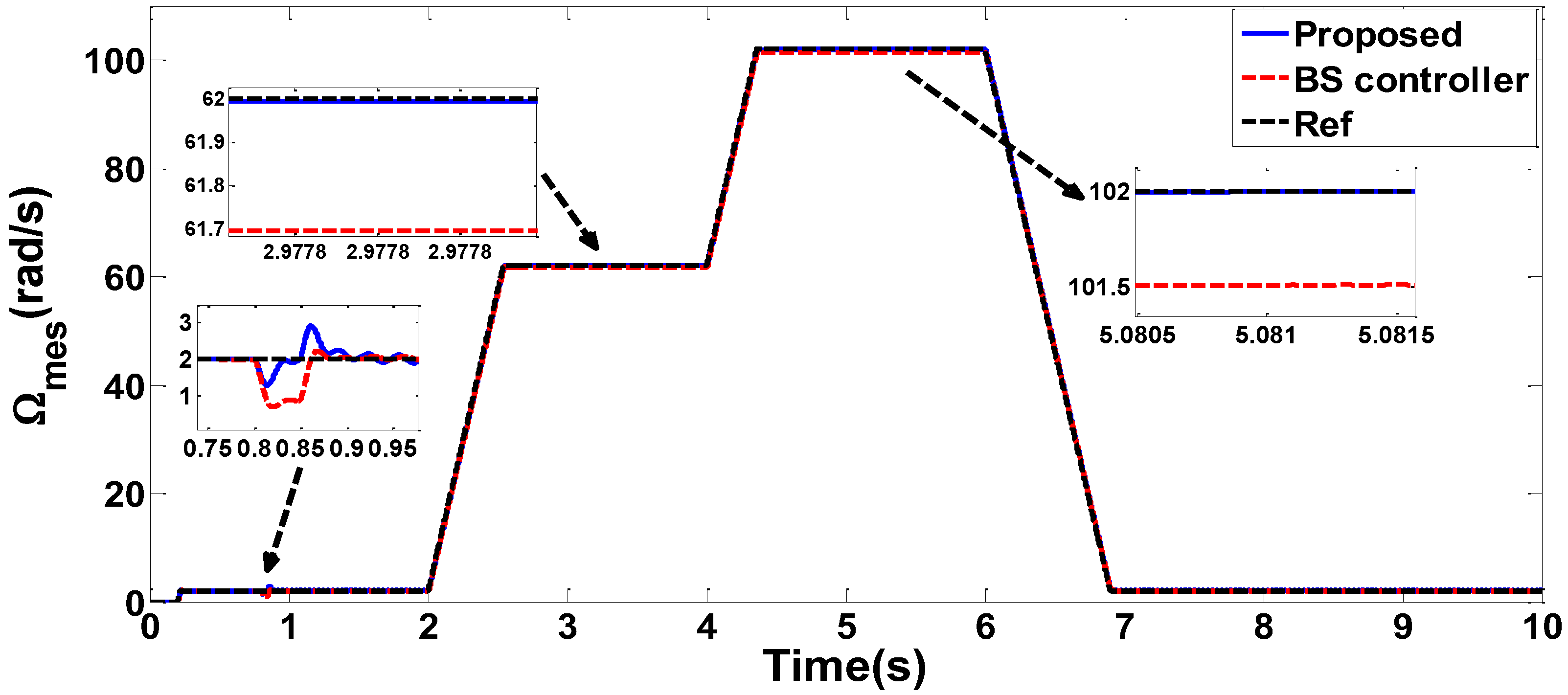
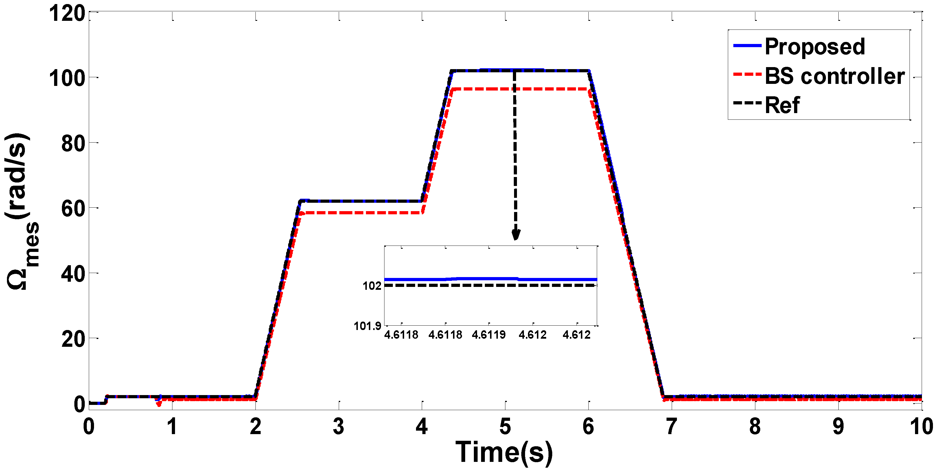
2.4. Simulation and Validaton

The performance of the suggested control strategy IBS-DISMC is performed in healthy operation mode and compared using the BSC approach reported in [13]. The physical parameters and the parameters of both controllers are respectively given in

Table 1. The parameters of the IM machine.

Parameters	Values
Rated output power	Pn = 1.2 kW
Rated speed	N = 1440 tr/min
Rated voltage	Vn = 220 V
Rated current	In = 6 A
Stator resistance	Rs = 1.8 Ω
Rotor resistance	Rr = 1.3 Ω
Stator inductances	Lls = 0.142 mH
Rotor inductances	Llr = 0.076 mH
Number of pole pairs	p = 2
Inertia load	J = 0.012 kg·m2
Viscous coefficient	f = 0.004 Nm/s

and

Table 2. The parameters of the reported approaches.

Item	Parameters
BS Controller	$k_{bsc1}=700$, $k_{bsc2}=170$, $k_{bsc3}=700$, $k_{bsc4}=170$
IBS-DISMC	$k_1=700$, $k_2=170$, $k_3=1200$, $k_4=2200$, $k_5=120$, $k_6=600$, and $k_{s1}=k_{s2}=20$
EKF	$Q=\left[\begin{array}{ccccc}1.533\begin{array}{c}e-12\end{array}& 0& 0& 0& 0\\ 0& 1.533\begin{array}{c}e-12\end{array}& 0& 0& 0\\ 0& 0& 1.873\begin{array}{c}e-8\end{array}& 0& 0\\ 0& 0& 0& 1.873\begin{array}{c}e-8\end{array}& 0\\ 0& 0& 0& 0& 67\begin{array}{c}e-1\end{array}\end{array}\right]$ $R=\left[\begin{array}{cc}1& 0\\ 0& 1\end{array}\right]$
SMO	$k_{smo1}=120$ and $k_{smo2}=20$

. For a chosen velocity profile and an applied step load torque of 2 Nm at t = 0.8 s, a simulation is carried out in closed loop. Figure 2 shows the response velocity of the suggested IBS-DISM and the BS controllers. Indeed, the velocity response using IBS-DISMC tracks the reference velocity with a very small steady-state error compared with the BSC.

In addition, a simulation is carried out to test the performance of both controllers in the presence of parameter variations, such as a variation of the IM stator winding resistance. Figure 3 presents the response velocities with the stator resistance variation of +25%. Indeed, the IBS-DISMC is quite insensitive to a large change in the machine resistance compared with the BSC.

3. Velocity Observers Design

Using observers for estimating the variable states of AC machines can be very useful. Interestingly, they act like redundant sensors which can be used in case of faults on analog or digital velocity sensors. Indeed, using observer increases the safety operation and reliability [28] and reduces both the cost maintenance and the machine size. In this study, an extended Kalman filter (EKF) and a sliding mode observer (SMO) are used to estimate the velocity of the IM. Both are designed using the analytical model of IM in the ($\alpha ,\beta$) reference frame. Therefore, the subscripts $\alpha$ and $\beta$ are added to the stator currents, fluxes, and voltages. In the next subsections, the mathematical structure of both observers will be studied. Additionally, discussions about why two observers are used will be highlighted.

3.1. Extended Kalman Filter

The EKF has been considered as a common estimation approach to estimate the velocity of the IM. Its algorithm consists of the following three steps: the prediction of the state vector, the Kalman filter gain computation, and the estimation of the state vector [7,29]:

Step one: Prediction

$$x_k^p=F{\widehat{x}}_{k-1}+B{u}_{k-1}$$

(25)

$$P_k^p=F{P}_{k-1}{F}^T+Q$$

(26)

Step two: Kalman filter gain calculation

$$K_k=P_k^p{H}^T{(H{P}_k^p{H}^T+R)}^{-1}$$

(27)

Step three: State vector estimation at time (k)

$${\widehat{x}}_k=x_k^p+K_k\left(y_k-H{x}_k^p\right)$$

(28)

$$\widehat{P}=\left(l-K_{k}H\right)P_k^p$$

(29)

Here, $x_k={[\begin{array}{ccccc}{i}_{s\alpha }& i_{s\beta }& {\psi }_{r\alpha }& {\psi }_{r\beta }& \Omega \end{array}]}^T$, $u_k={[\begin{array}{cc}{u}_{s\alpha }& u_{s\beta }\end{array}]}^T$, and $y_k={[\begin{array}{cc}{i}_{s\alpha }& i_{s\beta }\end{array}]}^T$. $Q$ and $R$ are the covariance matrix of state vector and the covariance matrix of measured output noise, respectively. $F$, $B$ and $H$ are given as follows [4,24]:

$$F=\left[\begin{array}{ccccc}{a}_{11}& b_{11}& a_{12}& b_{12}& f_1\\ -b_{11}& a_{11}& -b_{12}& a_{12}& f_2\\ a_{21}& b_{21}& a_{22}& b_{22}& f_3\\ -b_{21}& a_{21}& -b_{22}& a_{22}& f_4\\ 0& 0& 0& 0& 1\end{array}\right],B=\left[\begin{array}{cc}{a}_1& 0\\ 0& a_1\\ a_2& 0\\ 0& a_2\\ 0& 0\end{array}\right],H=\left[\begin{array}{ccccc}1& 0& 0& 0& 0\\ 0& 1& 0& 0& 0\end{array}\right]$$

$$\begin{gathered} a_{11}=1+\alpha T_s+\left({\alpha }^2+\beta \gamma \right)T_s^2/2 \\ {a}_{12}=\beta T_s\left(1+\left(\alpha +\delta \right)T_s/2\right)+c{\Omega }^2{T}_s{}^2/2 \\ {a}_{21}=\gamma T_s\left(1+\left(\alpha +\delta \right)T_s/2\right) \\ {a}_{22}=1+\delta T_s+\left({\delta }^2+\beta \gamma \right)T_s{}^2/2-{\Omega }^2{T}_s{}^2/2 \\ {b}_{11}=c\gamma \Omega T_s{}^2/2=-c{b}_{21} \\ {b}_{12}=(c{T}_s\left(1+\left(\alpha +\delta \right)T_s/2\right)-\beta T_s{}^2/2)\Omega \\ {b}_{21}=-\gamma \Omega T_s{}^2/2 \\ {b}_{22}=(-T_s+\left(c\gamma -2\delta \right)T_s{}^2/2)\Omega \\ {a}_1=\alpha T_s\left(1+\alpha T_s/2\right) \\ {a}_2=\alpha \gamma T_s{}^2/2 \\ {f}_1=0.5c\gamma T_s{}^2{x}_2\left(k\right)+c{T}_s{}^2{x}_5\left(k\right)x_3\left(k\right)+\left(c{T}_s\left(1+\left(\alpha +\delta \right)T_s/2\right)-\beta T_s{}^2/2\right)x_4\left(k\right) \\ {f}_2=-0.5c\gamma T_s{}^2{x}_1\left(k\right)+c{T}_s{}^2{x}_5\left(k\right)x_4\left(k\right)-\left(c{T}_s\left(1+\frac{\left(\alpha +\delta \right)T_s}{2}\right)-\frac{\beta T_s{}^2}{2}\right)x_3\left(k\right) \\ {f}_3=-0.5\gamma T_s{}^2{x}_2\left(k\right)-T_s{}^2{x}_5\left(k\right)x_3\left(k\right)+\left(0.5\left(c\gamma -2\delta \right)T_s{}^2-T_s\right)x_4\left(k\right) \\ {f}_4=0.5\gamma T_s{}^2{x}_1\left(k\right)-T_s{}^2{x}_5\left(k\right)x_4\left(k\right)-\left(0.5\left(c\gamma -2\delta \right)T_s{}^2-T_s\right)x_3\left(k\right) \end{gathered}$$

In the above equations, $T_s$ corresponds to the sampling time.

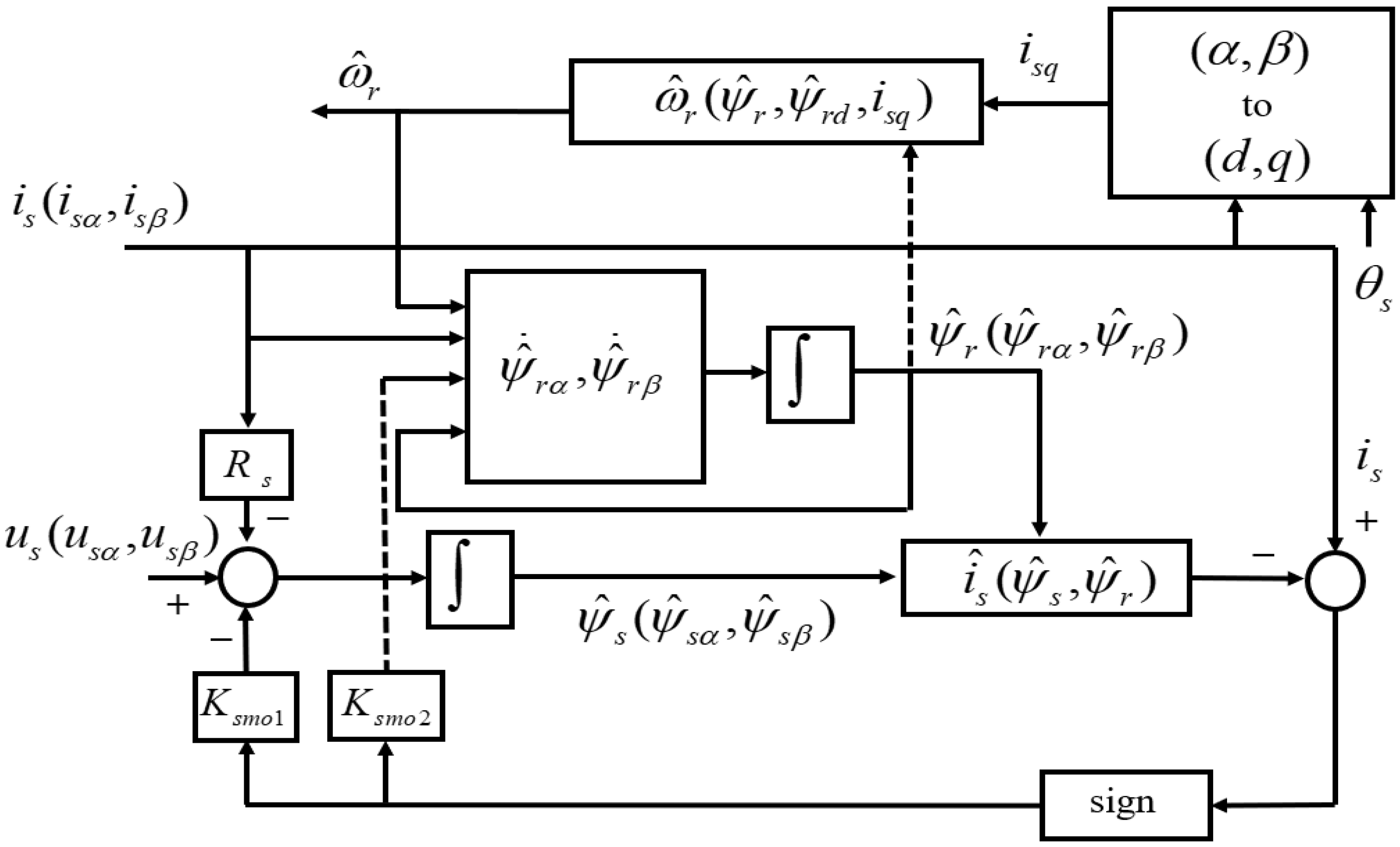
3.2. Sliding Mode Observer

A SMO is used to estimate the rotor velocity. Its algorithm can be easily implemented, and it has good performance even with process disturbance. Figure 4 gives the structure of the sliding mode observer to estimate the rotor velocity of the IM from the measured stator currents and voltages [30,31]:

The structure of the SMO given in Figure 4 is based on the following equations:

Stator flux:

$${\dot{\widehat{\psi }}}_{s\alpha }=u_{s\alpha }-R_s{i}_{s\alpha }-K_{smo1}{\Lambda }_{s\alpha }$$

(30)

$${\dot{\widehat{\psi }}}_{s\beta }=u_{s\beta }-R_s{i}_{s\beta }-K_{smo1}{\Lambda }_{s\beta }$$

(31)

Rotor flux:

$${\dot{\widehat{\psi }}}_{r\alpha }=\gamma i_{s\alpha }+\delta {\widehat{\psi }}_{r\alpha }-{\omega }_r{\widehat{\psi }}_{r\beta }+K_{smo2}{\Lambda }_{s\alpha }$$

(32)

$${\dot{\widehat{\psi }}}_{r\beta }=\gamma i_{s\beta }+\delta {\widehat{\psi }}_{r\beta }+{\omega }_r{\widehat{\psi }}_{r\alpha }+K_{smo2}{\Lambda }_{s\beta }$$

(33)

Stator currents:

$${\widehat{i}}_{s\alpha }=\left(1/\sigma L_s\right){\widehat{\psi }}_{s\alpha }-\left(\left(1-\sigma \right)/\left(\sigma L_{rs}\right)\right){\widehat{\psi }}_{r\alpha }$$

(34)

$${\widehat{i}}_{s\beta }=\left(1/\sigma L_s\right){\widehat{\psi }}_{s\beta }-\left(\left(1-\sigma \right)/\left(\sigma L_{rs}\right)\right){\widehat{\psi }}_{r\beta }$$

(35)

Estimated velocity:

$${\widehat{\omega }}_r=\frac{1}{{\widehat{\psi }}_{rd}{}^2}\left({\dot{\widehat{\psi }}}_{r\beta }{\widehat{\psi }}_{r\alpha }-{\dot{\widehat{\psi }}}_{r\alpha }{\widehat{\psi }}_{r\beta }\right)-\frac{L_{rs}}{T_r}\frac{i_{sq}}{{\widehat{\psi }}_{rd}}$$

(36)

where,

• ${\Lambda }_{s\alpha }=sign\left({\widehat{i}}_{s\alpha }-i_{s\alpha }\right)$, ${\Lambda }_{s\beta }=sign\left({\widehat{i}}_{s\beta }-i_{s\beta }\right)$, and ${\widehat{\psi }}_{rd}=\sqrt{{({\widehat{\psi }}_{r\alpha })}^2+{({\widehat{\psi }}_{r\beta })}^2}$. $K_{smo1}$ and $K_{smo2}$ are positive constants.

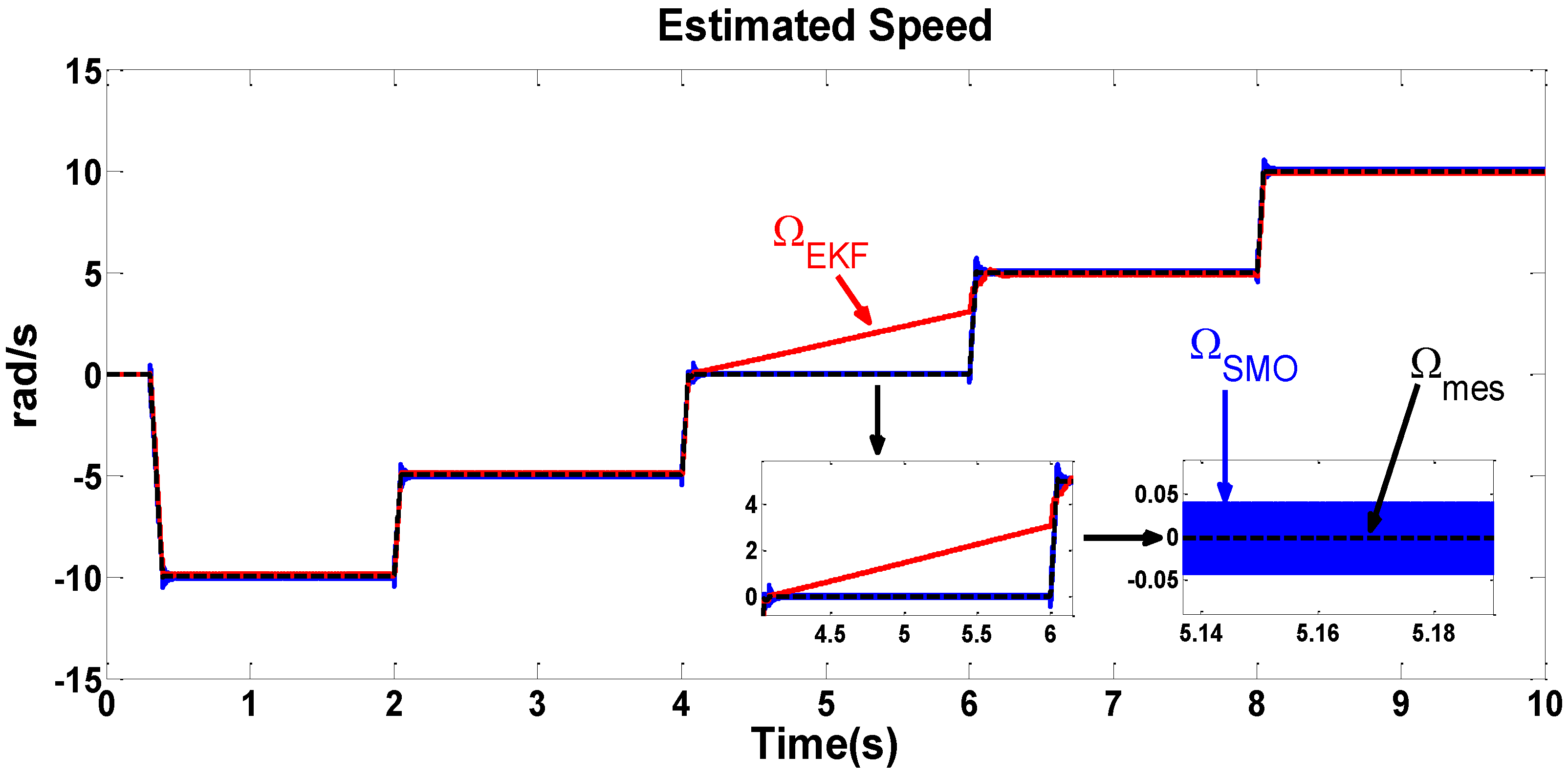
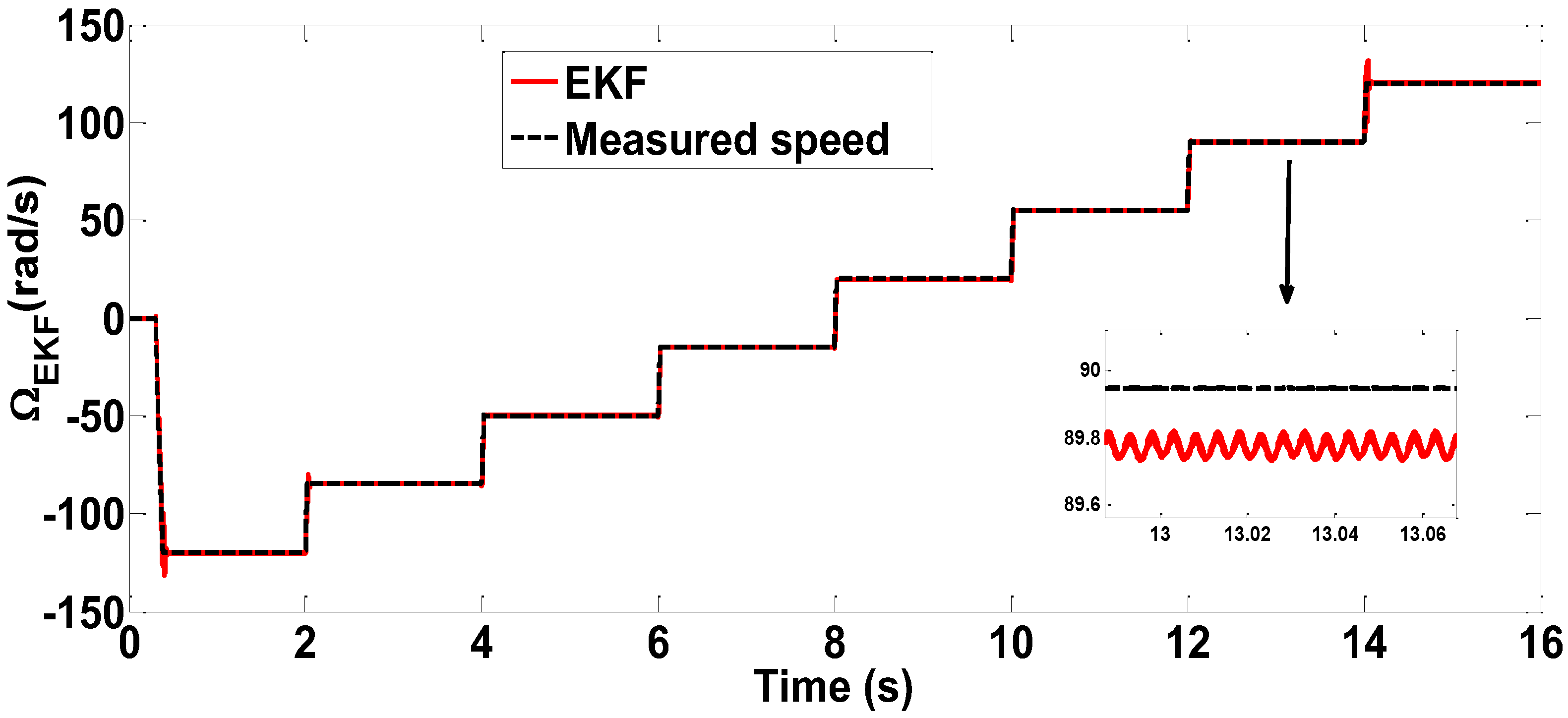
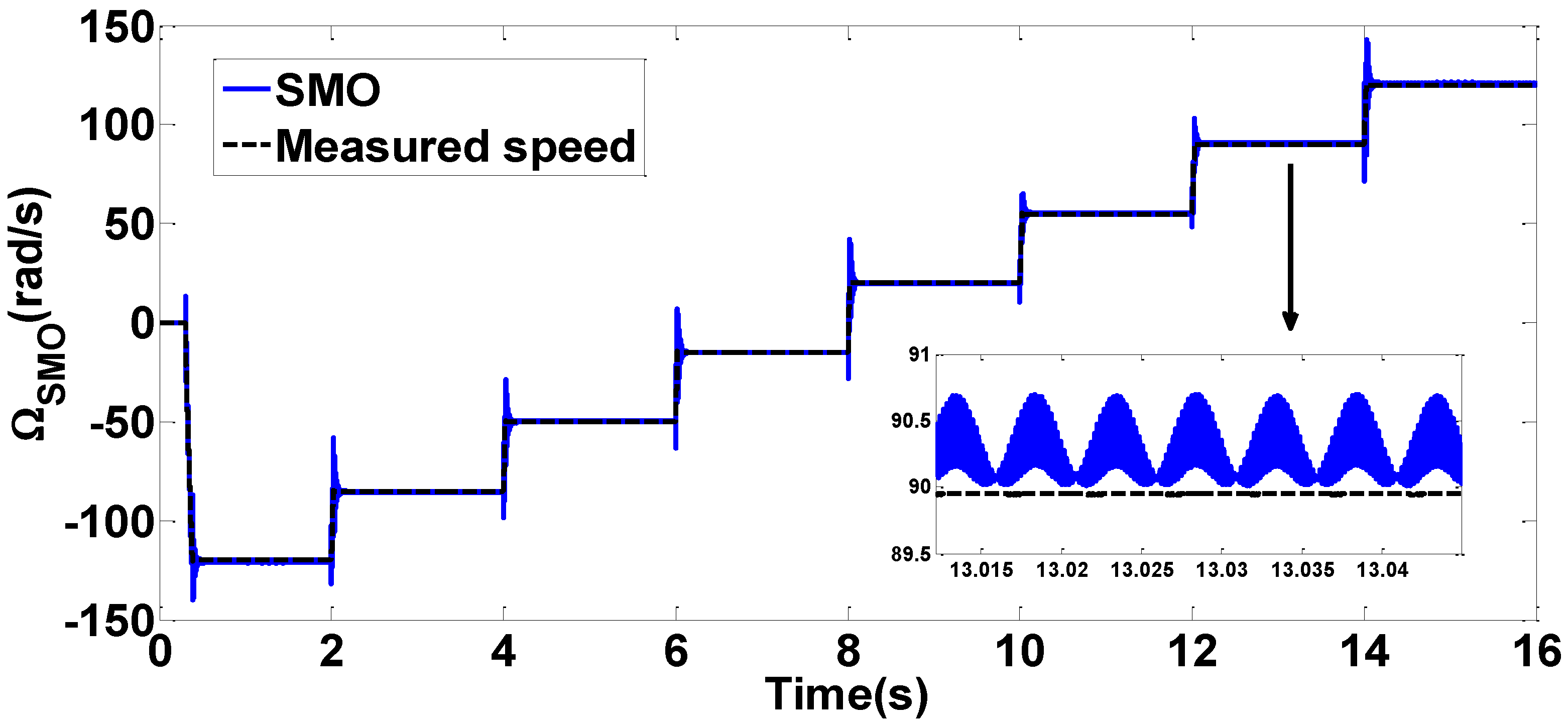
3.3. Simulation and Validation

Simulations are performed to evaluate the performance of the two observers, EKF and SMO, for all the velocity operating ranges with a nominal load. Figure 5 shows the performance of the two observers at low-velocity ranges. It is clear from the figure that EKF loses its observability at zero velocity, while SMO is stable at the same velocity.

Similarly, Figure 6 and Figure 7 show, respectively, the estimated velocity response of the IM using EKF and SMO at medium- and high-velocity operation ranges. Indeed, we can notice that EKF has a better performance compared with SMO. Figure 6 shows that EKF has no steady-state error and no overshot even with a velocity setpoint change, while in Figure 7, SMO suffers from overshoots and chattering. This phenomenon could be more important under process and sensor noises at high-velocity operation ranges. According to the above performance evaluation of EKF and SMO, the proposed FTC will use SMO for estimating low-range velocities, while it will use EKF for estimating medium- and high-range velocities. Both observers will only operate in faulty conditions. To clarify this point, the velocity physical sensor will be active for all the velocity operation ranges in healthy operation mode. On the other hand, SMO will be active at low-velocity operation ranges, and EKF at medium- and high-velocity operation ranges in faulty operation mode. A voting algorithm will be used to discover the faulty conditions and, accordingly, select either the physical velocity sensor or one of the two virtual observers to operate. It is also important to mention that the failure in the velocity sensor of the IM machine is assumed to be due to cable disconnection or power supply failure.

4. Fault-Tolerant Controller

The fault-tolerant control strategy suggested in this paper consistently maintains good performance of the velocity response in faulty operation mode using EKF and SMO. This combination is based on a voting algorithm that allows the selection of the best observer in faulty operation mode or the velocity sensor in healthy operation mode. Two approaches of voting algorithms are proposed and developed:

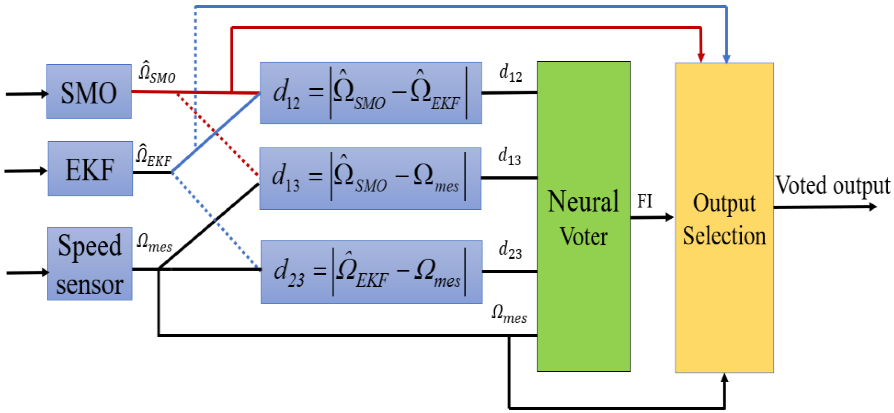
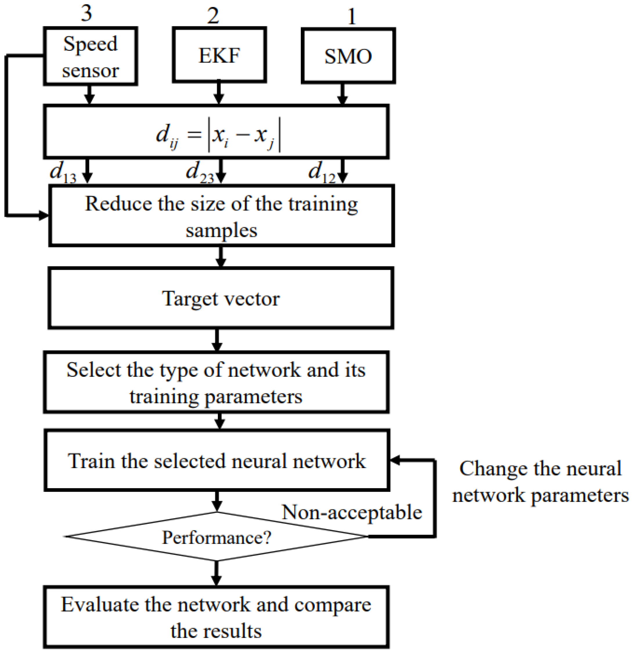
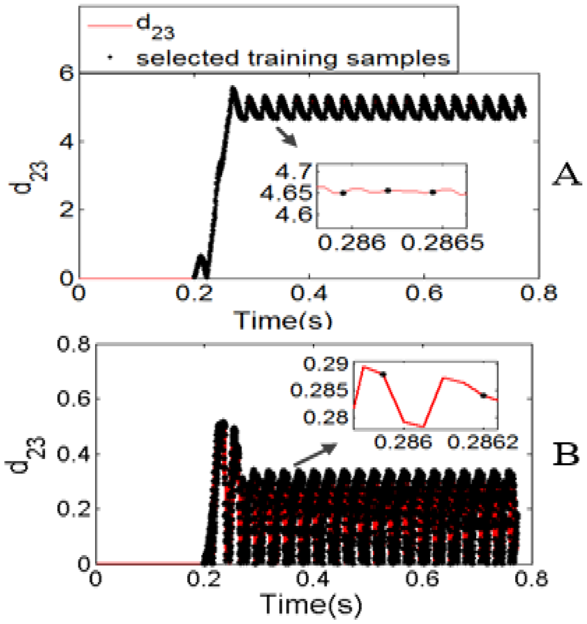
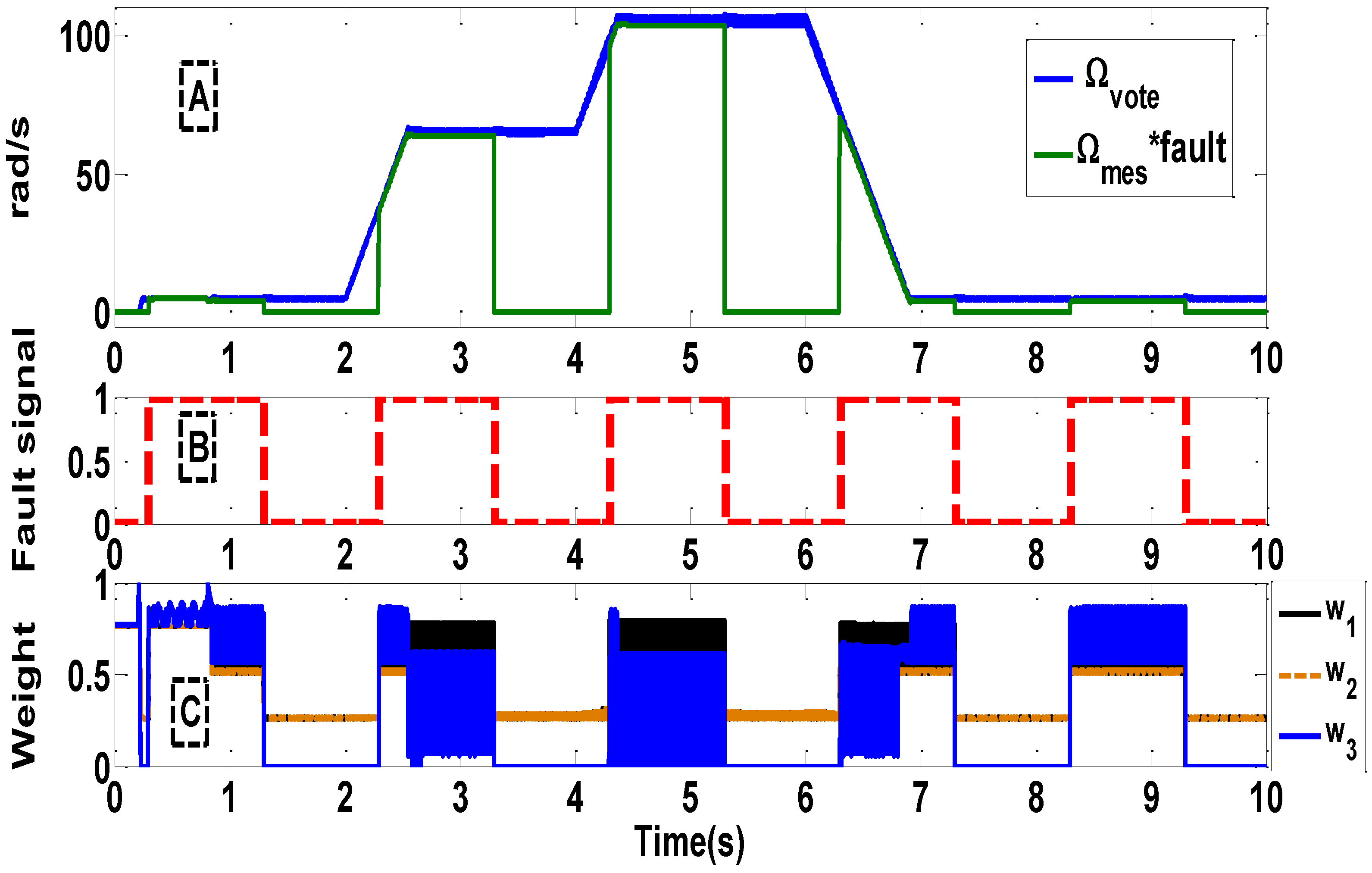
4.1. Neural Voter Algorithm

The key idea of the proposed neural voter (NV) is its ability to distinguish between healthy and faulty cases without the requirement of a predefined threshold value which directly affects the voter performance. The structure of the suggested voter is shown in Figure 8. The NV has four inputs and one output. Three of these inputs represent the distances obtained by calculating the difference between the estimated velocity of observers and the measured velocity as $d_{12}=\left|{\widehat{\Omega }}_{SMO}-{\widehat{\Omega }}_{EKF}\right|$, $d_{13}=\left|{\widehat{\Omega }}_{SMO}-{\Omega }_{mes}\right|$, and $d_{23}=\left|{\widehat{\Omega }}_{EKF}-{\Omega }_{mes}\right|$, respectively. These distances have the key feature of becoming relatively close to zero in the absence of fault, while they greatly differ from zero in the presence of fault. Thus, the neural voter could easily differentiate between normal and faulty operation modes. The fourth input of NV is the measured velocity. The output of NV is the fault indicator (FI) which takes two values, one or two, to indicate the healthy or the faulty operation mode.

The NV is trained to distinguish between healthy and faulty modes based on its previous training. The flowchart shown in Figure 9 presents the design phases of the NV, which diagnoses the mechanical sensor failure and selects the appropriate velocity from the two observers. In the first stage, the training samples, which are the vectors of the distances ($d_{12},d_{13},d_{23}$) and ${\Omega }_{mes}$, are generated in healthy and faulty modes for different values of velocities (2 rad/s, 5 rad/s, 10 rad/s, 20 rad/s, 70 rad/s, and 110 rad/s). In total, 12 scenarios will be used to train the neural network. For example, Figure 10 shows the selected training samples over the whole distance, $d_{23}$, in a faulty and healthy situation. Here, these samples are selected according to a defined step.

The size of samples is reduced to increase the efficiency of the neural network and to reduce the training time. In the second stage, the neural network is trained to differentiate between normal and abnormal conditions. Here, the target vector is assumed to have two values, one for a healthy sensor and two for a faulty sensor. The performances of different neural networks were evaluated in the third stage by checking the sum of squared error between the training and target vectors. As a result, the multilayer feed-forward back-propagation neural network with 2 layers (20 neurons in the hidden layer and a single neuron in the output layer) is selected. The settings of the neural network are determined to compromise between having small test errors and fewer computational burdens. Figure 11 shows the final structure of the neural network used.

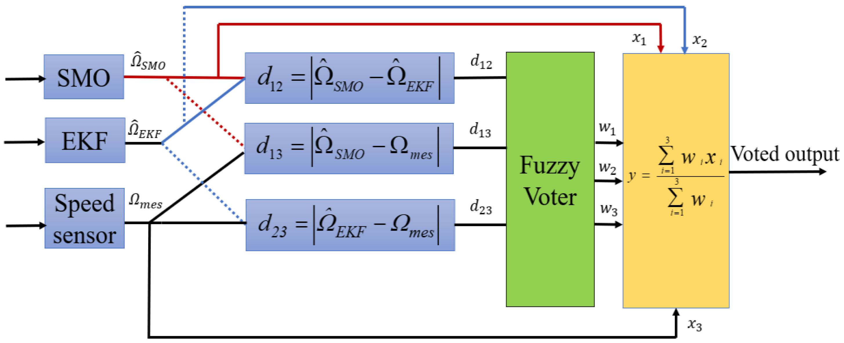
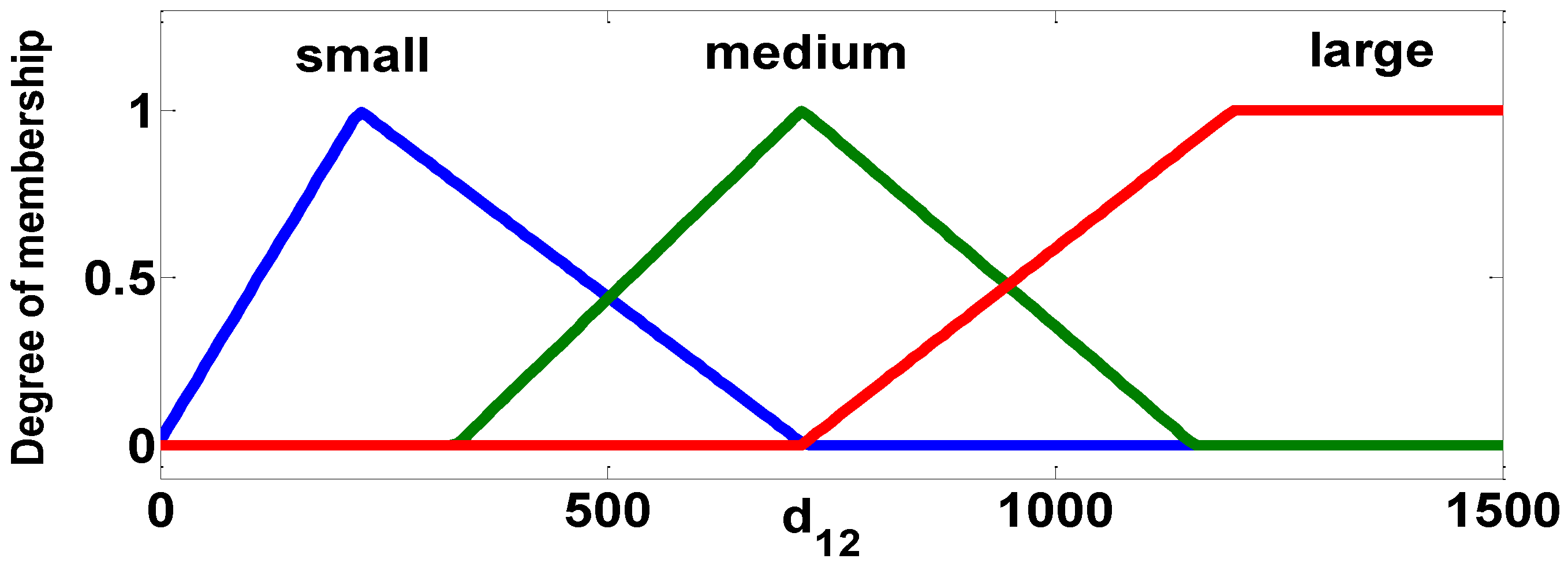
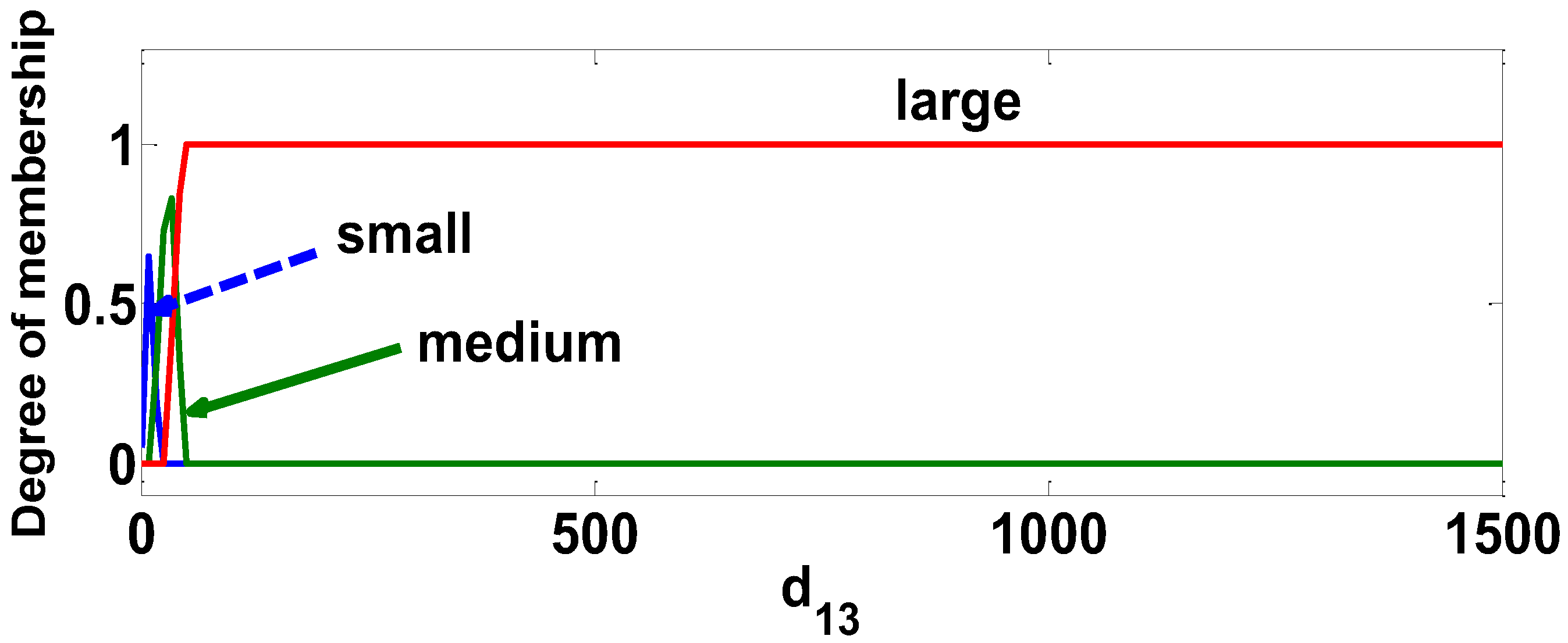
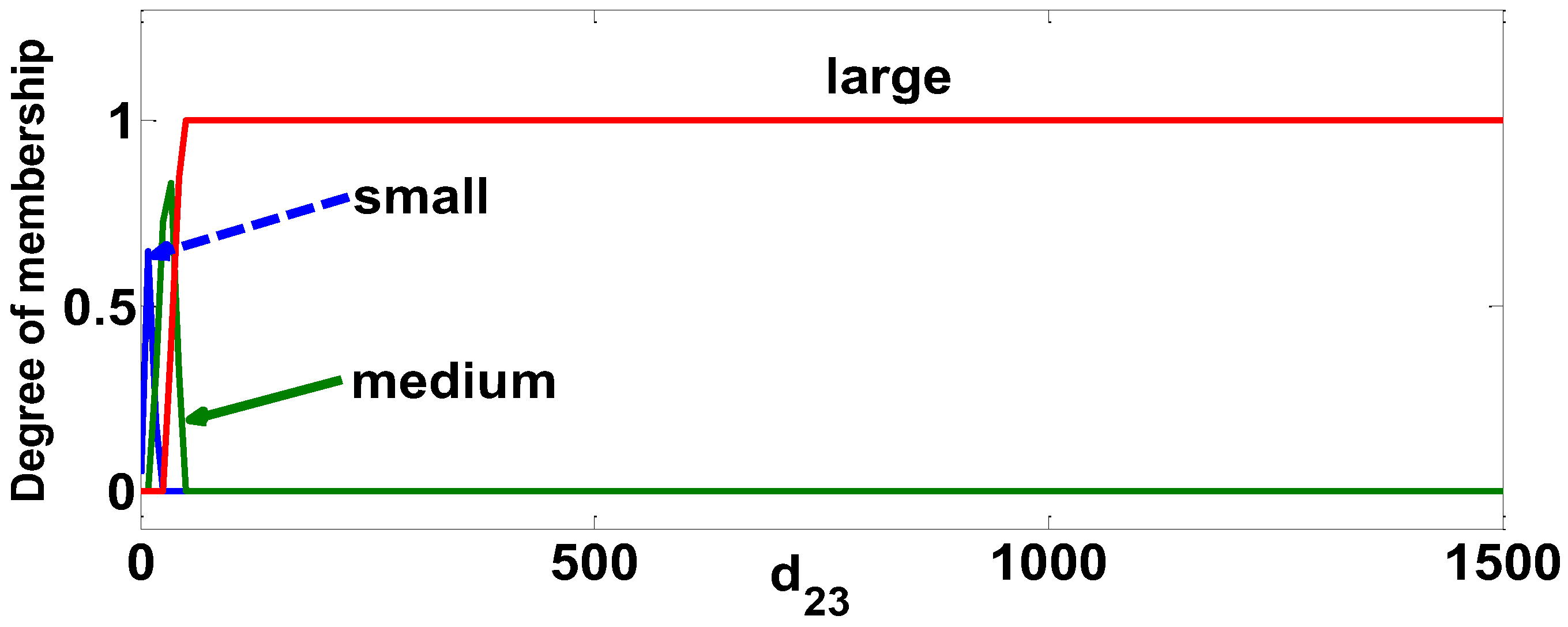
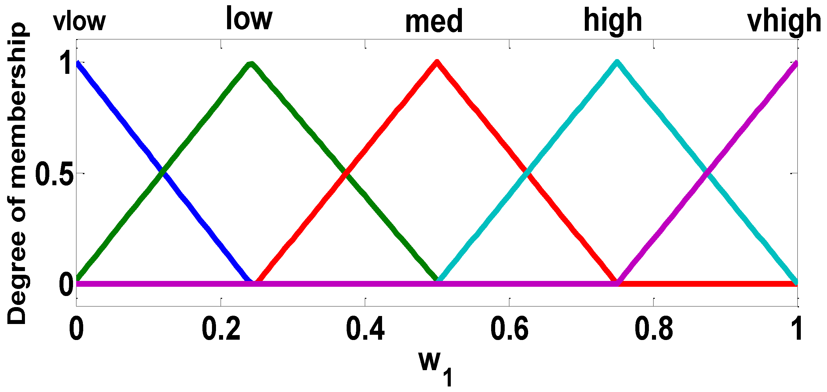
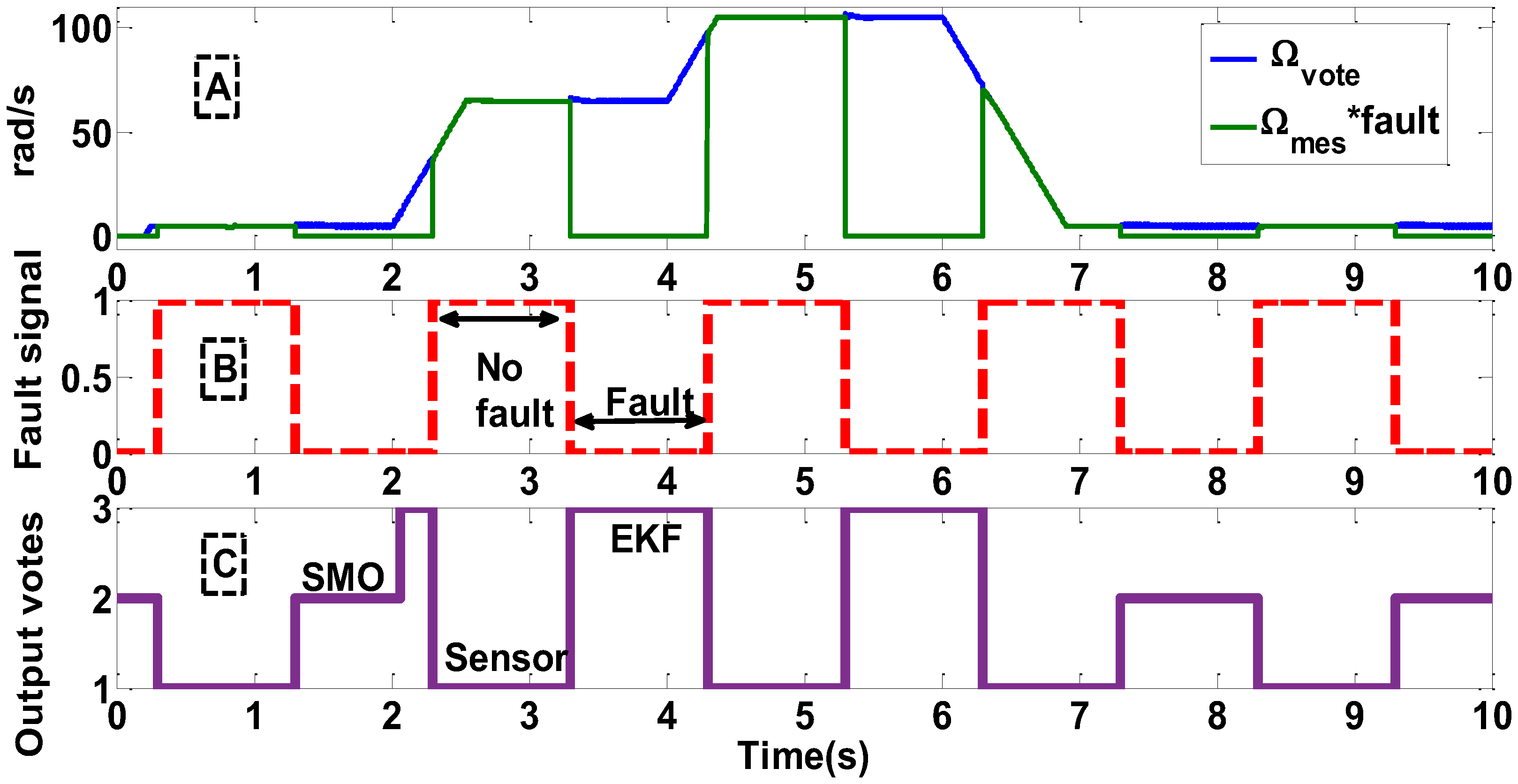
4.2. Fuzzy Voter Algorithm

The fuzzy voter uses fuzzy logic to produce the weights necessary for computing a weight average voter output [19]. In this study, the fuzzy voter is suggested and implemented in the structure of a sensor fault tolerant control for the IM machine. Its structure is shown in Figure 12, where $x_1$, $x_2$, and $x_3$ represent ${\widehat{\Omega }}_{SMO}$, ${\widehat{\Omega }}_{EKF}$, and ${\Omega }_{mes}$, respectively.

Figure 13, Figure 14 and Figure 15 represent the membership functions defined for the inputs $d_{12}=\left|{\widehat{\Omega }}_{SMO}-{\widehat{\Omega }}_{EKF}\right|,d_{13}=\left|{\widehat{\Omega }}_{SMO}-{\Omega }_{mes}\right|$ and $d_{23}=\left|{\widehat{\Omega }}_{EKF}-{\Omega }_{mes}\right|$, respectively.

According to the 3 inputs of the fuzzy voter, 27 fuzzy rules are defined for all the velocity operation ranges of the IM. The outputs w₁, w₂, and w₃ are defined as shown in Figure 16 by membership functions.

Finally using the following mathematical function, the final output of the fuzzy voter is computed:

$$y=\frac{{\displaystyle \sum _{i=1}^3}{w}_i·x_i}{{\displaystyle \sum _{i=1}^3}{w}_i}$$

(37)

Indeed, this value allows one to select SMO, or EKF, or the velocity sensor according to the operation mode and the operation velocity range.

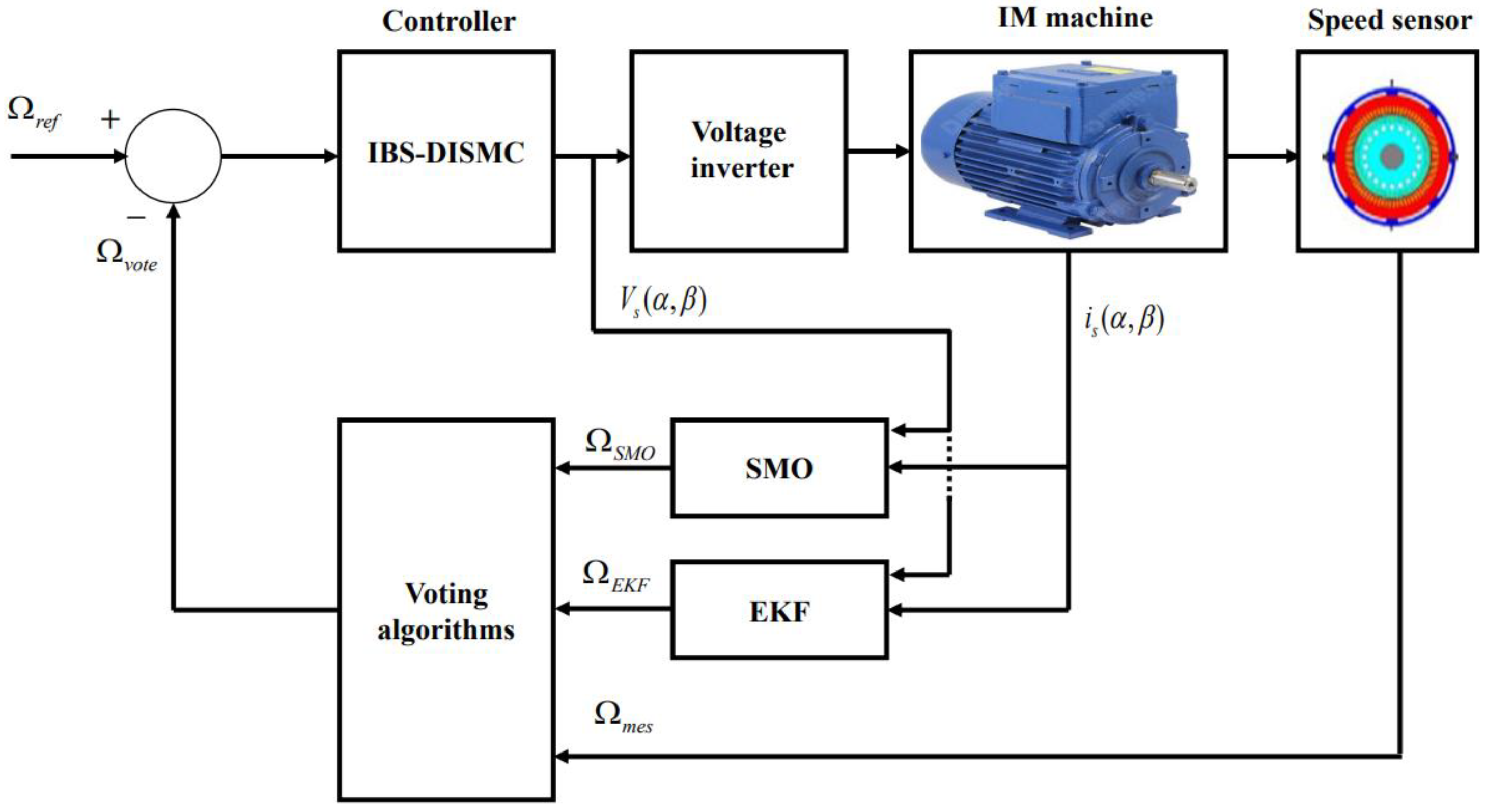
4.3. Fault-Tolerant Control Structure

The structure of the FTC, as shown in Figure 17, is based on the combination of the proposed controller IBS-DISMC, the two observers (EKF and SMO), and one of the suggested voting algorithms. In healthy operation mode, only the velocity sensor output is selected by the voting algorithm. However, in faulty operation mode and low-velocity operation, only SMO output is selected and, at medium- and high-velocity operation ranges only EKF, output is selected

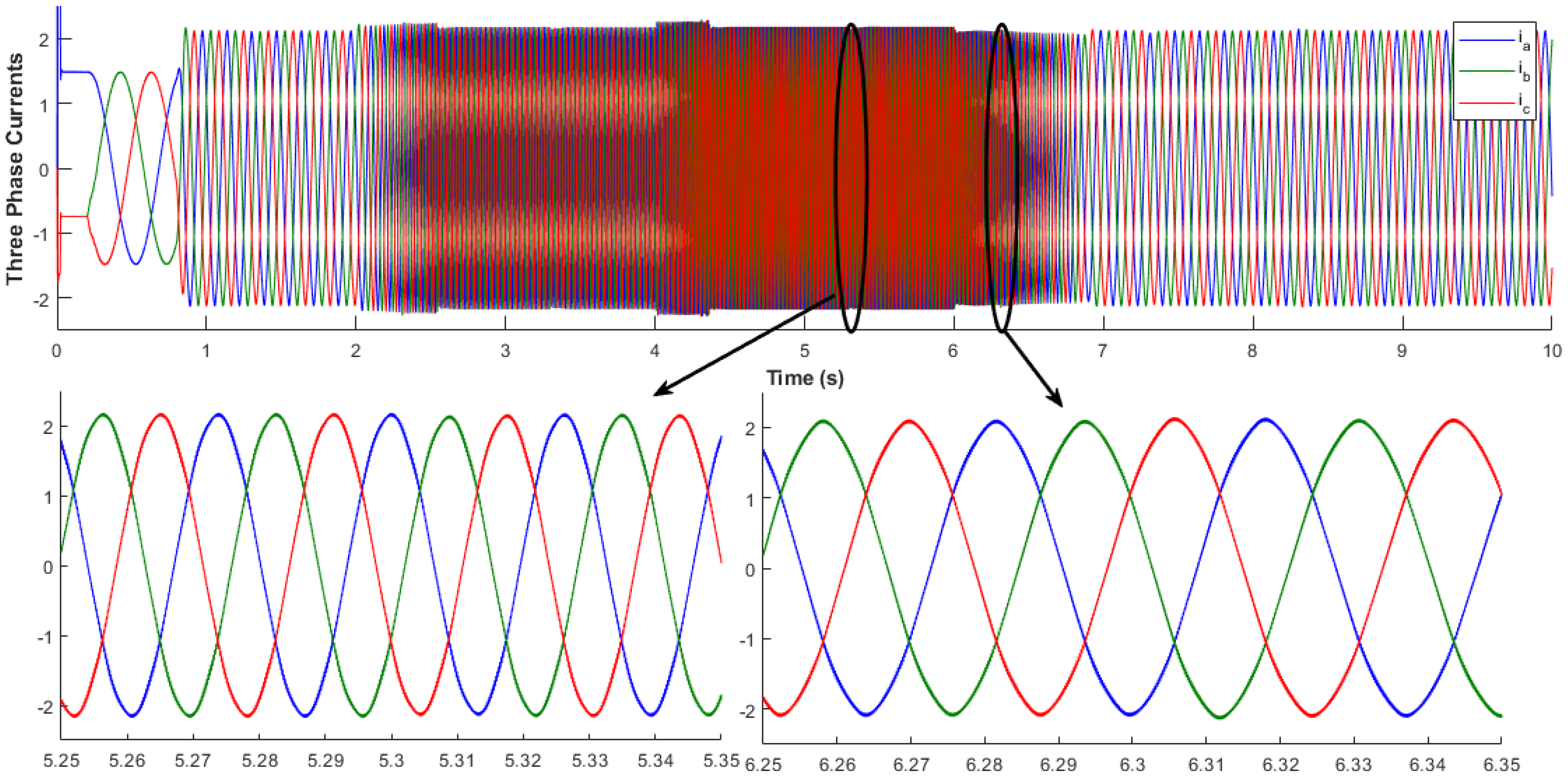
4.4. Simulation and Validation

The performance of the neural voting algorithm is compared with the fuzzy voter algorithm. Both voting algorithms are implemented separately using the FTC structure in Figure 17, where the detailed diagram of the IBS-DISMC controller was given in Figure 1. The proposed FTC was validated using MATLAB SIMULINK. In this simulation, it is assumed that the velocity sensor of the IM machine is temporarily disconnected due to cable disconnection or power supply failure. To evaluate the performance of both voters, a scenario of successive failures in the form of intermittent sensor connection is created and applied every two seconds. In addition, a load torque is applied at t = 0.8 s, with parameter variations (the stator resistance increased by 15%).

Figure 18 shows the results of the FTC where the neural voter algorithm is used. Figure 18A shows the velocity voted output of the proposed neural voter after applying the fault signal given in Figure 18B which changes between 1 (no fault) and 0 (fault). Indeed, in faulty operation modes, the neural voting algorithm isolates the fault and selects the appropriate observer according to the velocity operation range. Figure 18C shows the response velocity, where SMO is selected at low velocities and EKF at medium and high velocities.

Similarly, Figure 19 shows the simulation results of the FTC where the fuzzy voter algorithm is used. Figure 19A shows that FV identifies failures, but it mixes between the estimated speeds of both observers at medium- and high-velocity ranges. This is mainly due to the evaluation of the mathematical relation given in (37), where the voter output is generated after the defuzzification of all the inputs.

Therefore, the neural voter has significantly improved the performance, compared to the fuzzy voter. Indeed, NV does not merge the estimated velocities, and its feasibility has been proven in case of a sensor failure. In addition, NV does not require the setting of a threshold, while the fuzzy voter requires adjusting numerous numbers of thresholds (membership functions). Figure 20 represents the three phase stator currents where neither oscillations nor spikes are observed during the switching modes of the neural voter algorithm.

5. Conclusions

The proposed fault-tolerant control strategy has the potential to improve the performance of the induction machine and increase the reliability and safety of both healthy and faulty operation modes. The suggested structure of FTC is based on the combination of a vector controller, two observers, and a voting algorithm, which selects the appropriate estimated velocity of the SMO and EKF observers in case of a mechanical sensor failure. The FTC was developed by incorporating a new controller and a new voting algorithm. Simulation results show that the proposed controller has greater performance relative to the BS controller. Additionally, these results ensure that the proposed voting algorithm offers better performance compared to the fuzzy voter. Indeed, the proposed voter based on artificial intelligence overcomes the difficulty of setting the voter threshold correctly. Moreover, it only selects a single input to generate the voter output. On the other hand, the fuzzy voter produces its output by averaging its inputs. This means that the faulty sensor still contributes to the voter output, and this may lead to an unstable system in a real-time scenario. In addition, it requires the adjustment of multiple thresholds, which is time-consuming. For future studies, this work will be followed by an experimental validation on an existing test bench of an induction machine. Additionally, the effects of unbalance currents and voltages on the accuracy of estimated velocities by the SMC and EKF will be investigated. Moreover, reducing the chattering of the SMO will be the core of our future works.

References

1. Akrad, A.; Hilairet, M.; Diallo, D. Design of a Fault-Tolerant Controller Based on Observers for a PMSM Drive. IEEE Trans. Ind. Electron. 2011, 58, 1416–1427. [Google Scholar] [CrossRef]
2. Tousizadeh, M.; Che, H.S.; Selvaraj, J.; Rahim, N.A.; Ooi, B.T. Performance Comparison of Fault-Tolerant Three-Phase Induction Motor Drives Considering Current and Voltage Limits. IEEE Trans. Ind. Electron. 2019, 66, 2639–2648. [Google Scholar] [CrossRef]
3. Fekih, A.; Mobayen, S.; Chen, C.C. Adaptive robust fault-tolerant control design for wind turbines subject to pitch actuator faults. Energies 2021, 16, 1791. [Google Scholar] [CrossRef]
4. Rotondo, D. Background on Fault Tolerant Control. In Advances in Gain-Scheduling and Fault Tolerant Control Techniques; Springer: Berlin/Heidelberg, Germany, 2018. [Google Scholar]
5. Amin, A.; Hasan, K. A review of fault tolerant control systems: Advancement and applications. Measurement 2019, 143, 58–68. [Google Scholar] [CrossRef]
6. Hasan, M.; Haris, M.; Qin, S. Fault-tolerant spacecraft attitude control: A critical assessment. Prog. Aerosp. Sci. 2022, 130, 100806. [Google Scholar] [CrossRef]
7. Raisemche, A.; Boukhnifer, M.; Larouci, C.; Diallo, D. Two active fault-tolerant control schemes of induction-motor drive in EV or HEV. IEEE Trans. Veh. Technol. 2014, 63, 19–29. [Google Scholar] [CrossRef]
8. Garramiola, F.; Olmo, J.D.; Poza, J.; Madina, P.; Almandoz, G. Integral Sensor Fault Detection and Isolation for Railway Traction Drive. Sensors 2018, 18, 1543. [Google Scholar] [CrossRef] [PubMed] [Green Version]
9. Berzoy, A.; Mohammed, O.A.; Restrepo, J. Analysis of the Impact of Stator Inter-Turn Short-Circuit Faults on Induction Machines driven by Direct Torque Control. IEEE Trans. Energy Convers. 2018, 33, 1463–1474. [Google Scholar] [CrossRef]
10. Hajary, S.A.; Kianinezhad, R.; Seifossadat, S.G.; Mortazavi, S.S.; Saffarian, A. Detection and Localization of Open-phase Fault in Three Phase Induction Motor Drives using Second Order Rotational Park Transformation. IEEE Trans. Power Electron. 2019, 34, 11241–11252. [Google Scholar] [CrossRef]
11. Najafabadi, T.A.; Salmasi, F.R.; Jabehdar-Maralani, P. Detection and isolation of speed-, DC-link voltage-, and current-sensor faults based on an adaptive observer in induction-motor drives. IEEE Trans. Ind. Electron. 2011, 58, 1662–1672. [Google Scholar] [CrossRef]
12. Morel, C.; Akrad, A.; Sehab, R.; Azib, T.; Larouci, C. Open-Circuit Fault-Tolerant Strategy for Interleaved Boost Converters via Filippov Method. Energies 2022, 15, 352. [Google Scholar] [CrossRef]
13. Alyoussef, F.; Akrad, A. Speed Sensor Fault-Tolerant Controller for Induction Motor Using New Minimum Probability Voter Based on Signal Strength. In Proceedings of the 2019 International Conference on Applied Automation and Industrial Diagnostics (ICAAID), Elazig, Turkey, 25–27 September 2019. [Google Scholar]
14. Yu, Y.; Wang, Z.; Xu, D.; Zhou, T.; Xu, R. Speed and Current Sensor Fault Detection and Isolation Based on Adaptive Observers for IM Drives. J. Power Electron. 2014, 14, 967–979. [Google Scholar] [CrossRef]
15. Tabbache, B.; Benbouzid, M.; Kheloui, A. On the Transition Improvement of EV or HEV Induction Motor Propulsion Sensor Fault-Tolerant Controller. In Proceedings of the IEEE Vehicle Power and Propulsion Conference, Lille, France, 1–3 September 2010. [Google Scholar]
16. Chakraborty, C.; Verma, V. Speed and current sensor fault detection and isolation technique for induction motor drive using axes transformation. IEEE Trans. Ind. Electron. 2015, 62, 1943–1954. [Google Scholar] [CrossRef]
17. Choi, C.; Lee, K.; Lee, W. Observer-based phase-shift fault detection using adaptive threshold for rotor position sensor of permanent-magnet synchronous machine drives in electromechanical brake. IEEE Trans. Ind. Electron. 2015, 62, 1964–1974. [Google Scholar] [CrossRef]
18. Lorczak, P.R.; Caglayan, A.K.; Eckhardt, D.E. A theoretical investigation of generalized voters for redundant systems. In Proceedings of the Nineteenth International Symposium on Fault-Tolerant Computing, Chicago, IL, USA, 21–23 June 1989. [Google Scholar]
19. Latif-Shabgahi, G.; Hirst, A.J. A fuzzy voting scheme for hardware and software fault tolerant systems. Fuzzy Sets Syst. 2005, 150, 579–598. [Google Scholar] [CrossRef]
20. Leung, Y.W. Maximum Likelihood Voting for Fault-Tolerant Software with Finite Output-Space. IEEE Trans. Reliab. 1995, 44, 419–427. [Google Scholar] [CrossRef]
21. Raisemche, A.; Boukhnifer, M.; Diallo, D. New fault-tolerant control architectures based on voting algorithms for electric vehicle induction motor drive. Trans. Inst. Meas. Control. 2016, 38, 1120–1135. [Google Scholar] [CrossRef]
22. Lin, F.J.; Wai, R.J.; Chou, W.D.; Hsu, S.P. Adaptive backstepping control using recurrent neural network for linear induction motor drive. IEEE Trans. Ind. Electron. 2002, 49, 134–146. [Google Scholar]
23. Soto, R.; Yeung, K.S. Sliding-mode control of an induction motor without flux measurement. IEEE Trans. Ind. Appl. 1995, 31, 744–751. [Google Scholar] [CrossRef]
24. Jia, Z.; Yu, J.; Mei, Y. Integral backstepping sliding mode control for quadrotor helicopter under external uncertain disturbances. Aerosp. Sci. Technol. 2017, 68, 299–307. [Google Scholar] [CrossRef]
25. Adhikary, N.; Mahanta, M. Integral backstepping sliding mode control for underactuated systems: Swing-up and stabilization of the Cart-Pendulum System. ISA Trans. 2013, 52, 870–880. [Google Scholar] [CrossRef] [PubMed]
26. Qureshi, M.A.; Ahmad, I.; Munir, M.F. Double integral sliding mode control of continuous gain four quadrant quasi-z-source converter. IEEE Access 2018, 6, 77785–77795. [Google Scholar] [CrossRef]
27. Pradhan, R.; Subuddhi, B. Double Integral Sliding Mode MPPT Control of a Photovoltaic System. IEEE Trans. Control. Syst. Technol. 2016, 24, 285–292. [Google Scholar] [CrossRef]
28. Vas, P. Sensorless Vector and Direct Torque Control; Oxford University Press: London, UK, 1998. [Google Scholar]
29. Hilairet, M.; Auger, F.; Berthelot, E. Speed and rotor flux estimation of induction machines using a two-stage extended Kalman filter. Automatica 2009, 45, 1819–1827. [Google Scholar] [CrossRef]
30. Lascu, C.; Boldea, I.; Blaabjerg, F. A class of speed-sensorless sliding-mode observers for high-performance induction motor drives. IEEE Trans. Ind. Electron. 2009, 56, 3394–3403. [Google Scholar] [CrossRef]
31. Yang, J.; Zhu, F.; Wang, X.; Bu, X. Robust sliding-mode observer-based sensor fault estimation, actuator fault detection and isolation for uncertain nonlinear systems. Int. J. Control Autom. Syst. 2015, 13, 1037–1046. [Google Scholar] [CrossRef]
Figure 1. Diagram of the suggested IBS-DISMC.
Energies 15 03084 g001
Figure 2. Velocity responses of the induction machine using BSC and IBS-DISMC.
Energies 15 03084 g002
Figure 3. Velocity responses of the induction machine using BSC and IBS-DISMC for a stator winding resistance change of +25%.
Energies 15 03084 g003
Figure 4. SMO structure.
Energies 15 03084 g004
Figure 5. Estimated speed of EKF and SMO at low-velocity operation range.
Energies 15 03084 g005
Figure 6. Estimated velocity response using of EKF at medium- and high-velocity operation ranges.
Energies 15 03084 g006
Figure 7. Estimated velocity response using of SMO at medium- and high-velocity operation ranges.
Energies 15 03084 g007
Figure 8. Structure of the Neural Voter Algorithm.
Energies 15 03084 g008
Figure 9. The flowchart of the NV.
Energies 15 03084 g009
Figure 10. Training samples: (A) in a faulty mode, (B) in a healthy mode.
Energies 15 03084 g010
Figure 11. The structure of the multilayer feed-forward back-propagation neural network.
Energies 15 03084 g011
Figure 12. The structure of the fuzzy voter.
Energies 15 03084 g012
Figure 13. Membership functions for the distance d 12 .
Energies 15 03084 g013
Figure 14. Membership functions for the distance d 13 .
Energies 15 03084 g014
Figure 15. Membership functions for the distance d 23 .
Energies 15 03084 g015
Figure 16. Membership functions for the outputs w 1 ,   w 2   and   w 3 .
Energies 15 03084 g016
Figure 17. FTC structure.
Energies 15 03084 g017
Figure 18. (A) The output of the proposed voting algorithm, (B) Applied fault signal, (C) Selected speed (1: sensor, 2: SMO, 3: EKF).
Energies 15 03084 g018
Figure 19. (A) The output of the fuzzy voting algorithm, (B) The applied fault signal, (C) The weights of the fuzzy voter.
Energies 15 03084 g019
Figure 20. Stator currents for the neural voter.
Energies 15 03084 g020