
An Operation Strategy of ESS for Enhancing the Frequency Stability of the Inverter-Based Jeju Grid


Abstract
:1. Introduction
2. Modeling and Methods
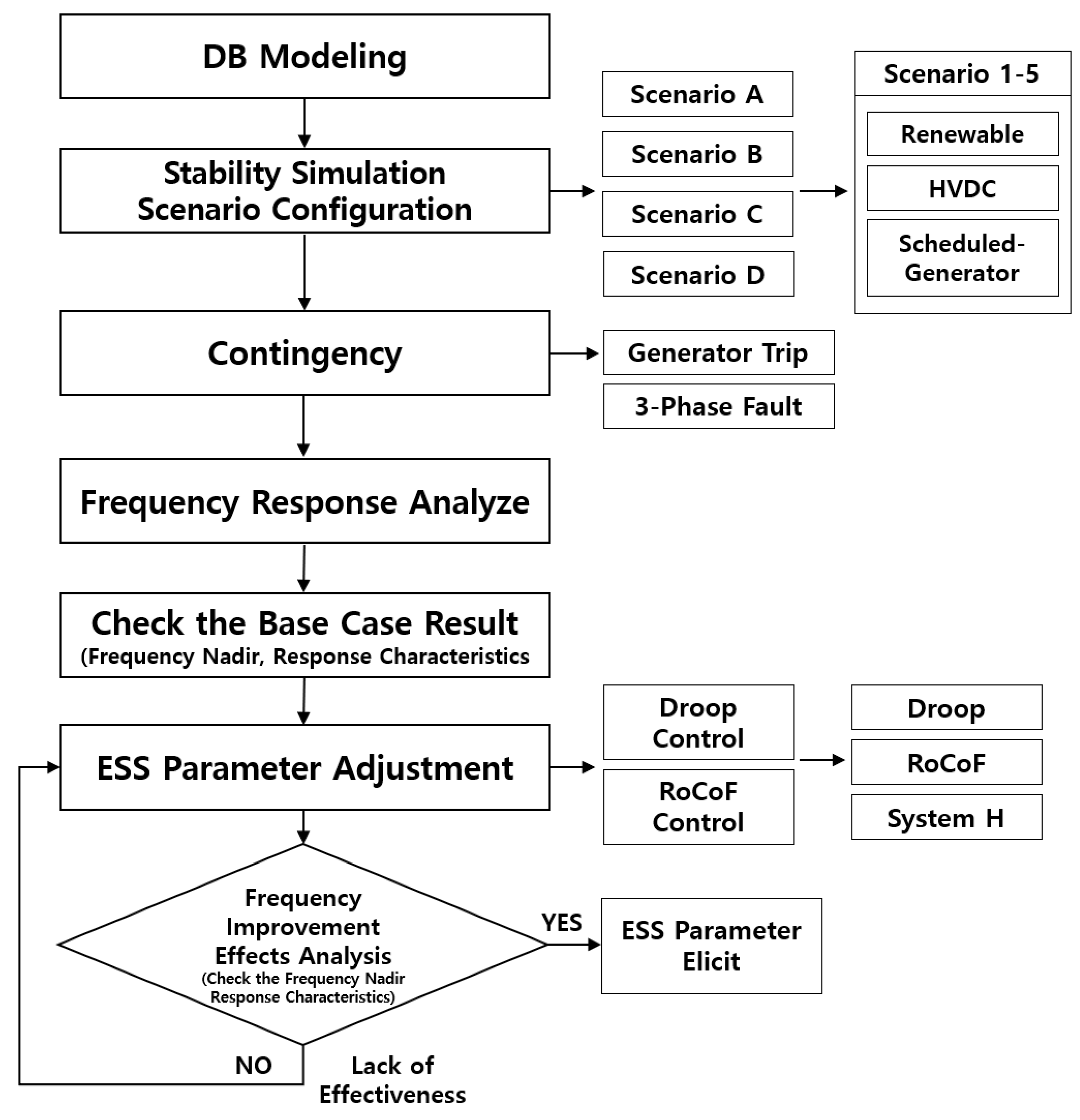
2.1. Frequency Stability Simulation Methods
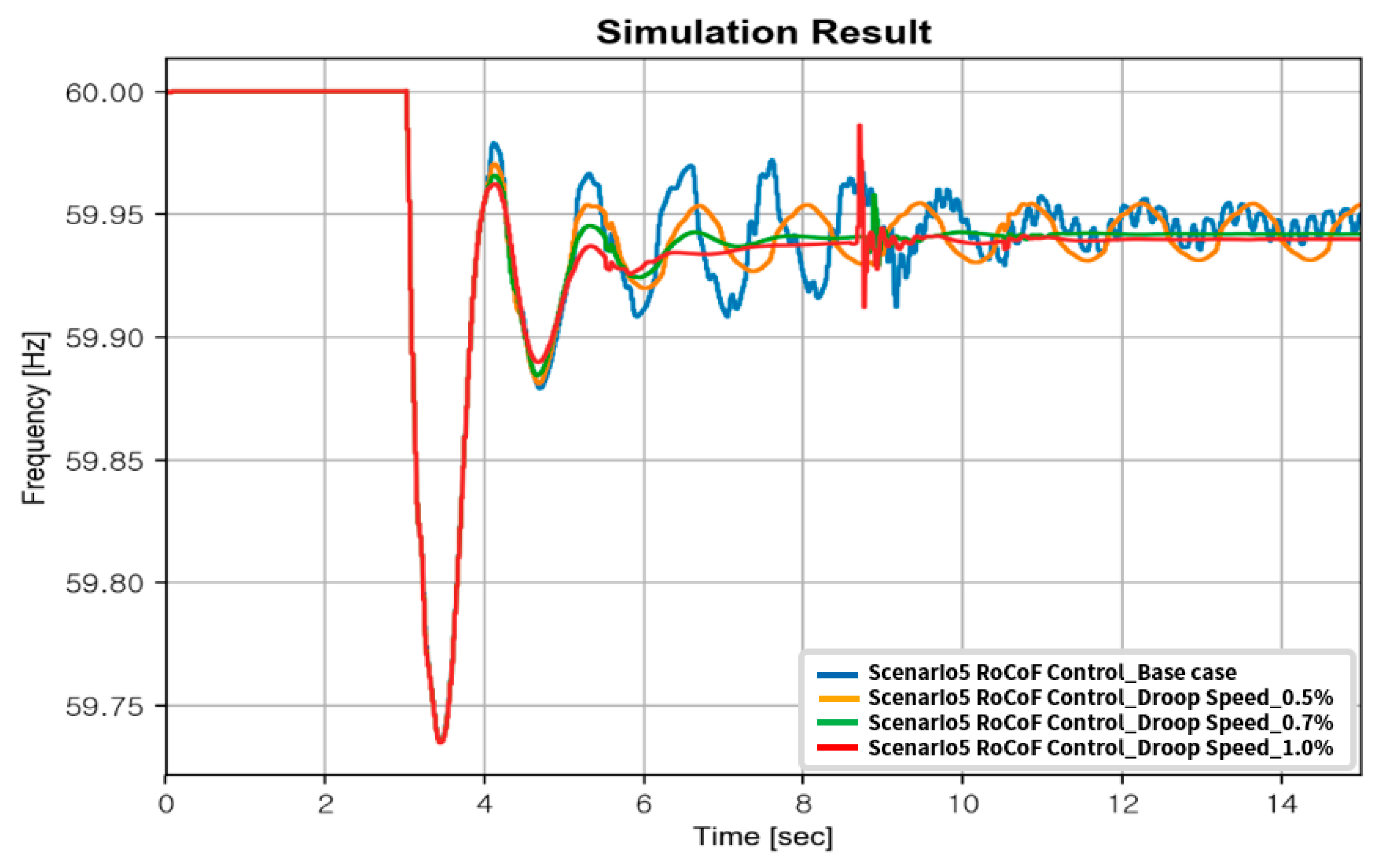
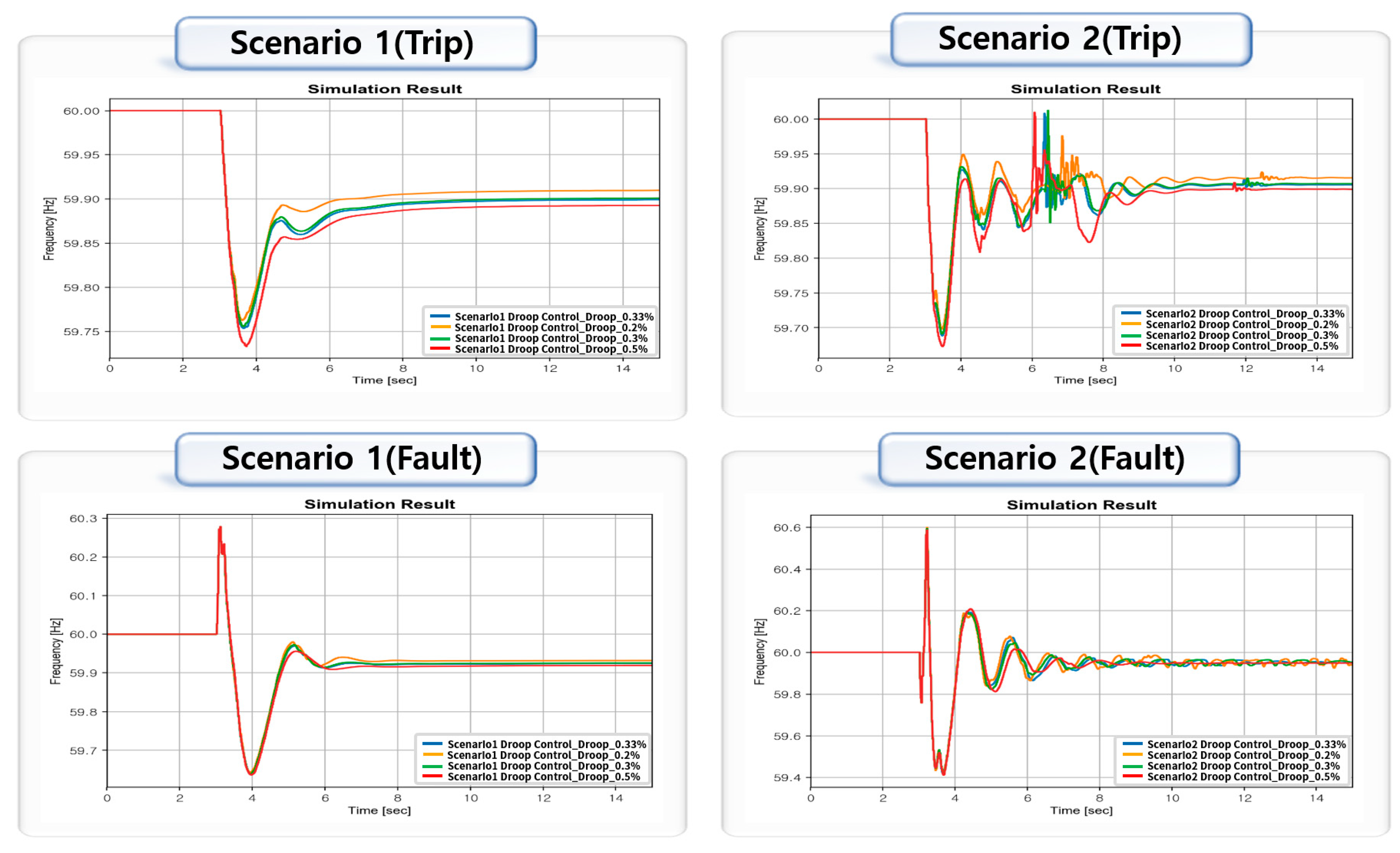
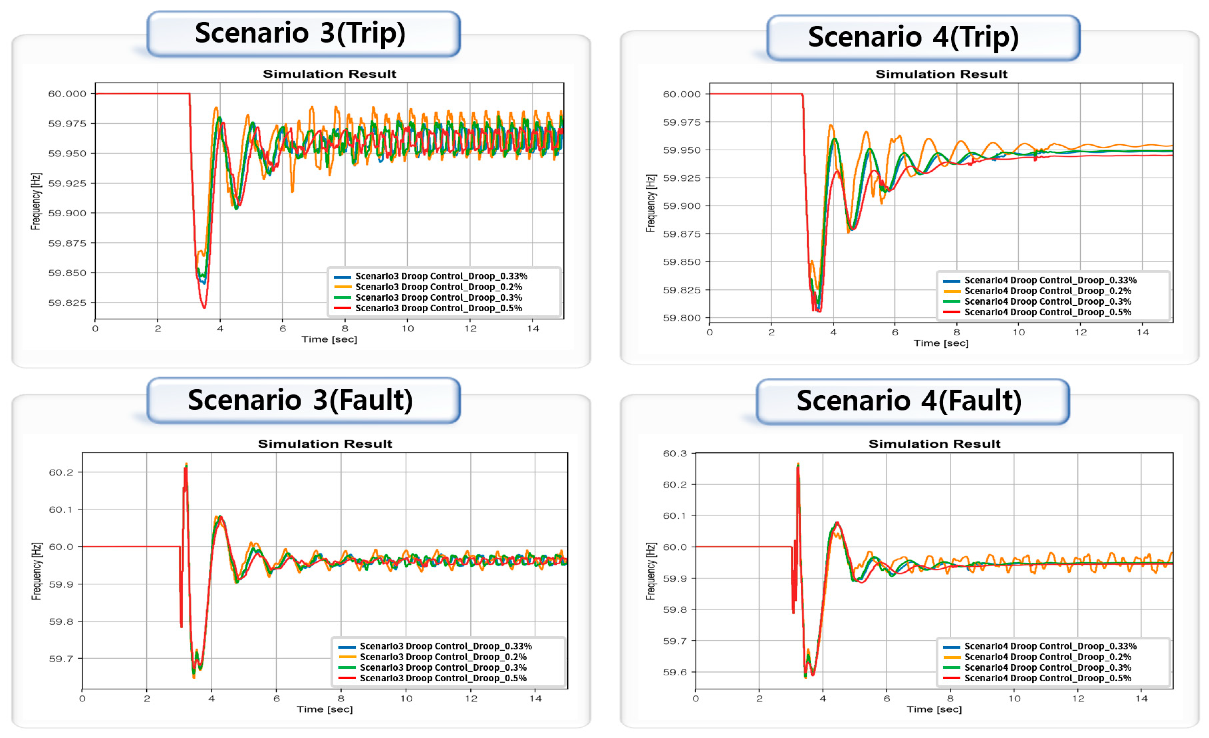
- ESS Droop control.
- ○
- Droop speed.
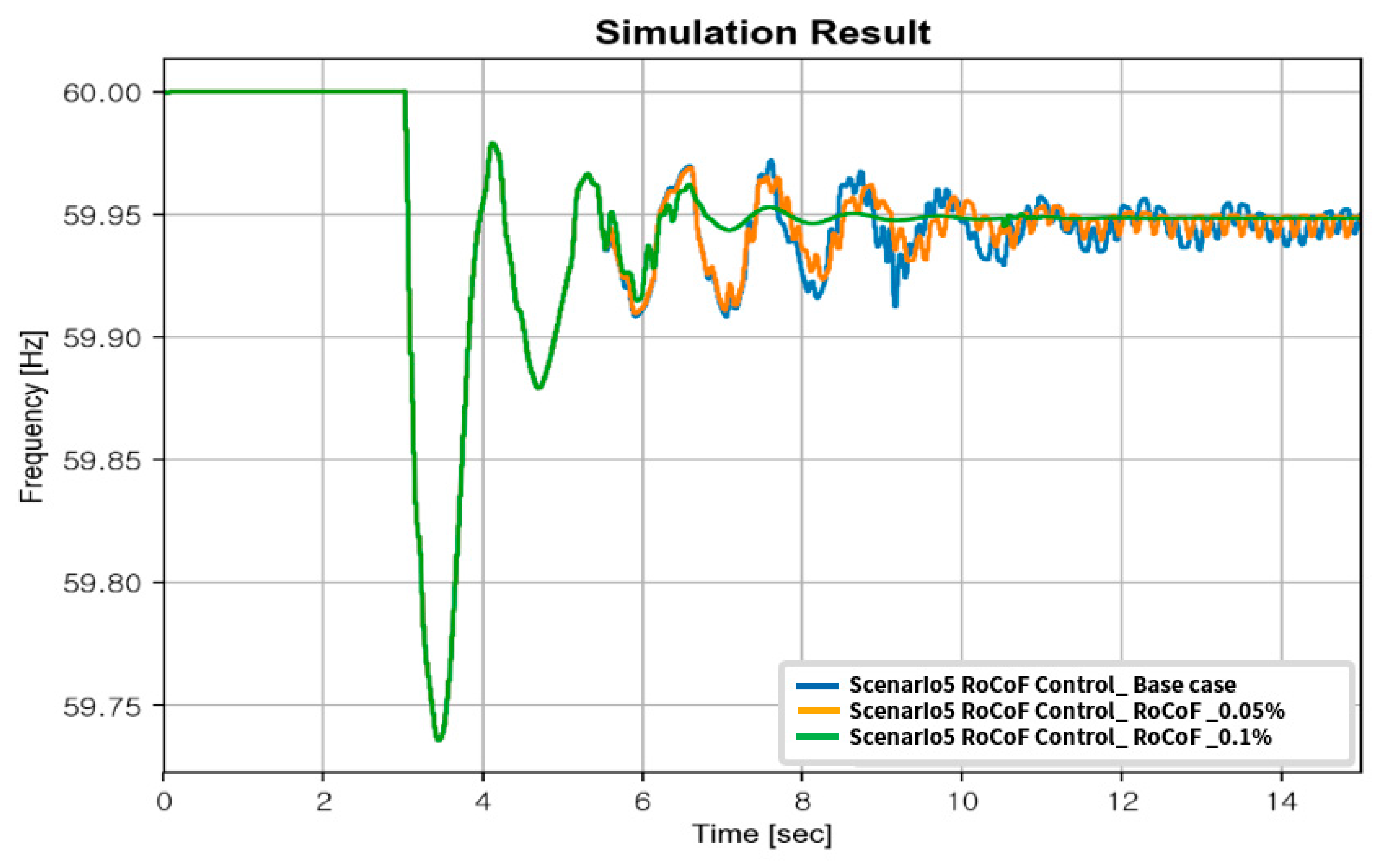
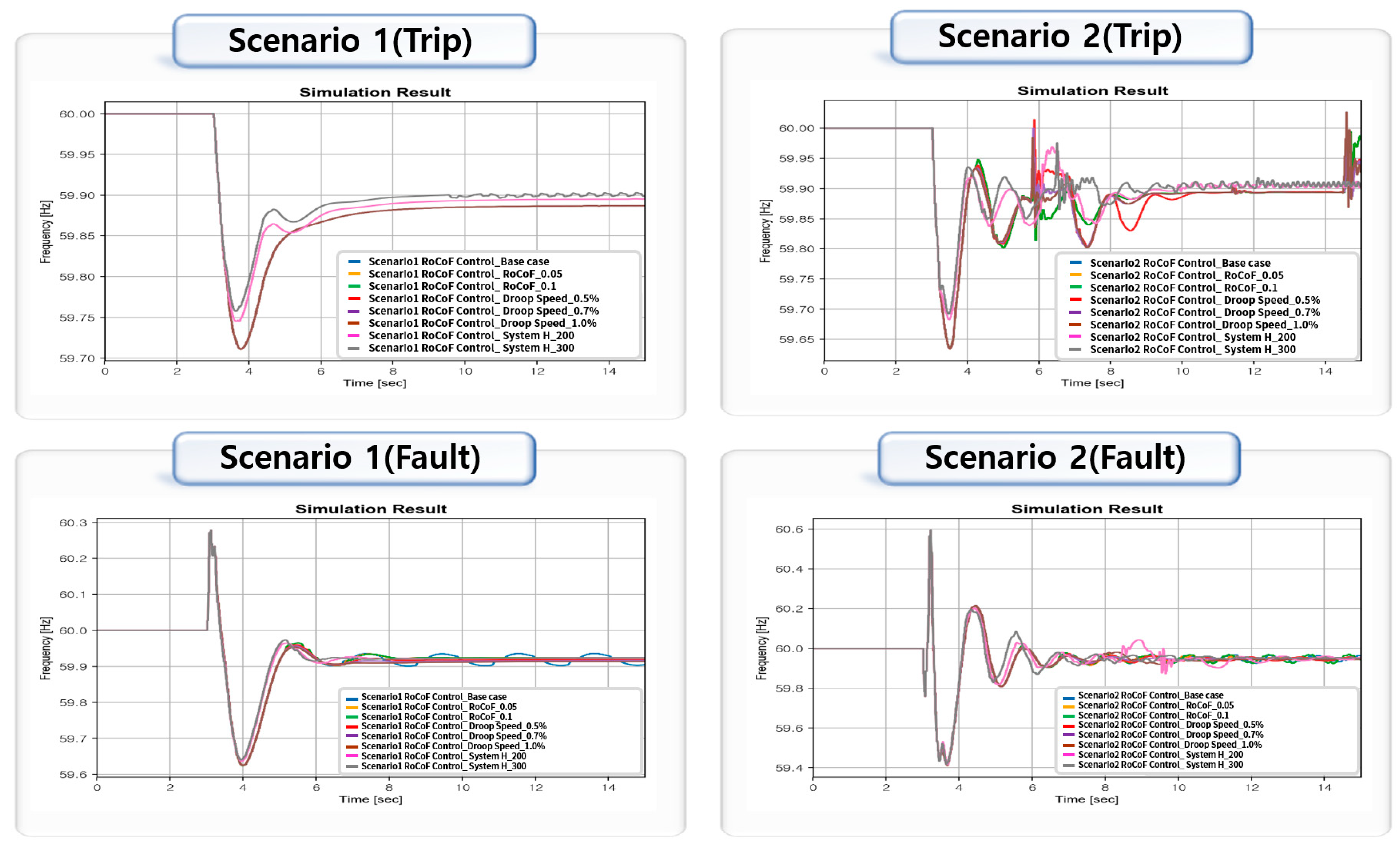
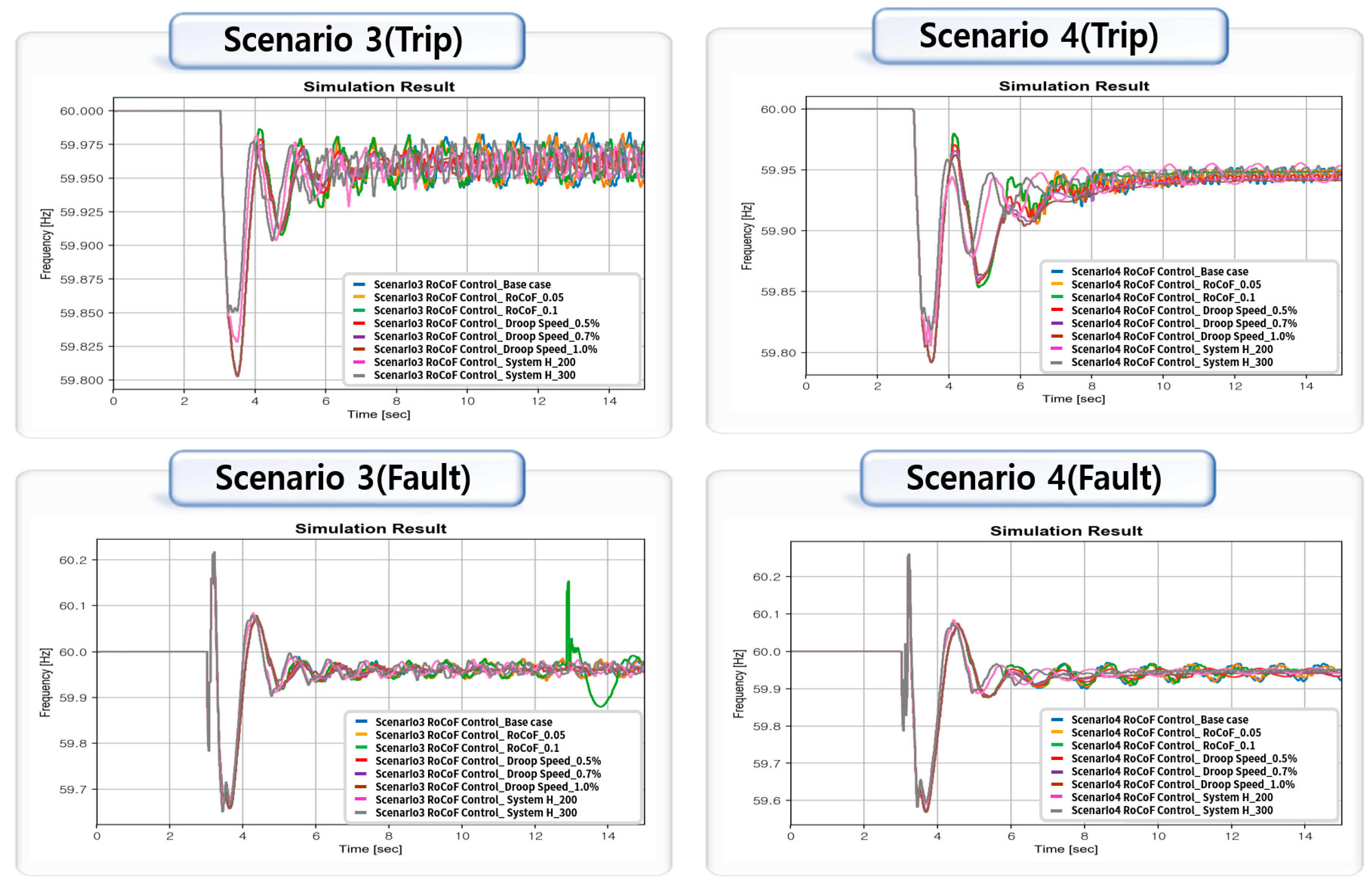
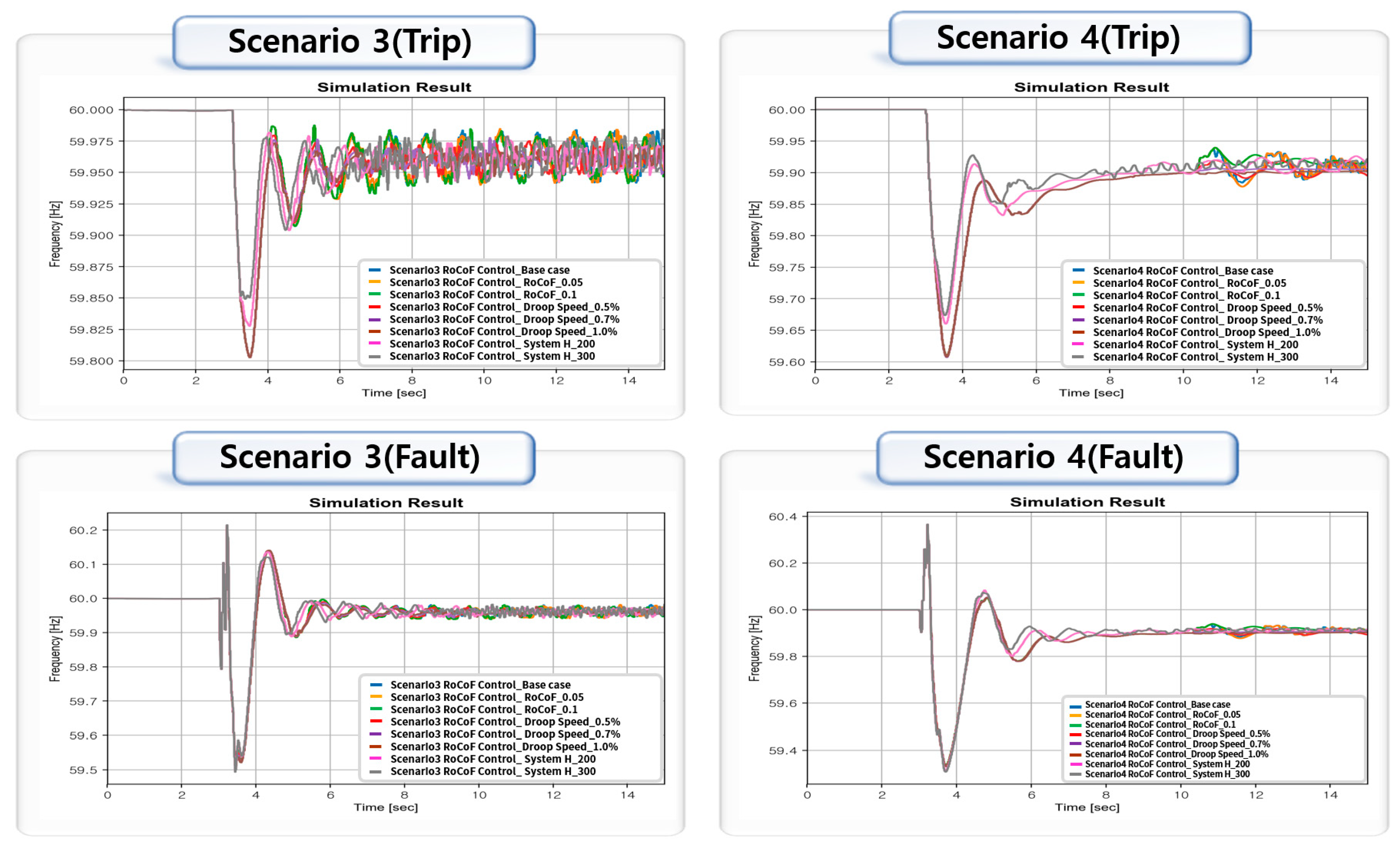
- ESS RoCoF control.
- ○
- Dead band.
- ○
- RoCoF for trans-state (trans-state judgement RoCoF).
- ○
- Droop for steady-state and trans-recovery.
- ○
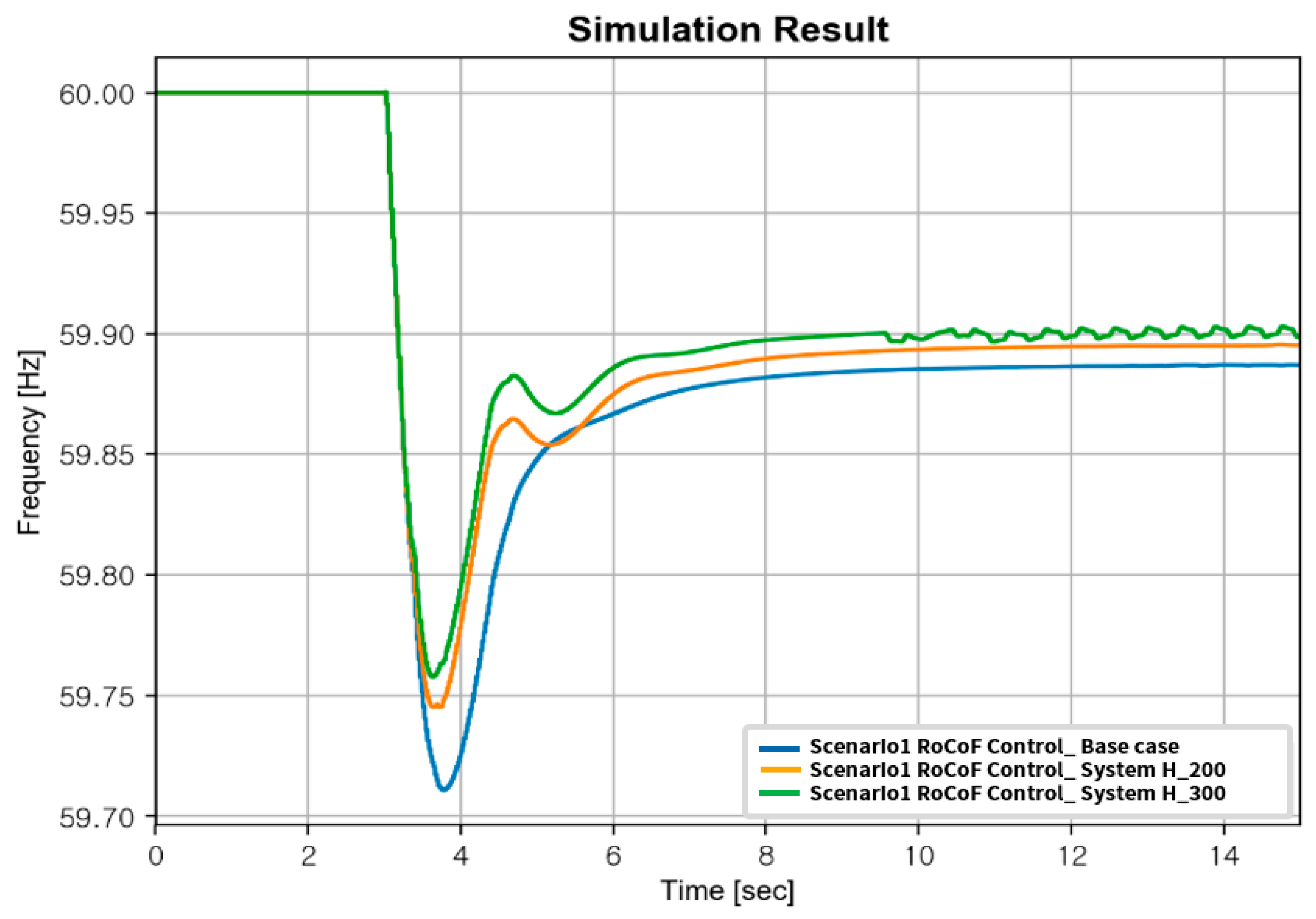
- System H for trans-state (ESS output).
2.2. Scenario Configuration
- Scenario A,B,C: classification according to HVDC No.3 operation characteristics and the model.
- Scenario 1–5: classification according to the renewable power generation and HVDC circulation operation.
- Five must-run generators.
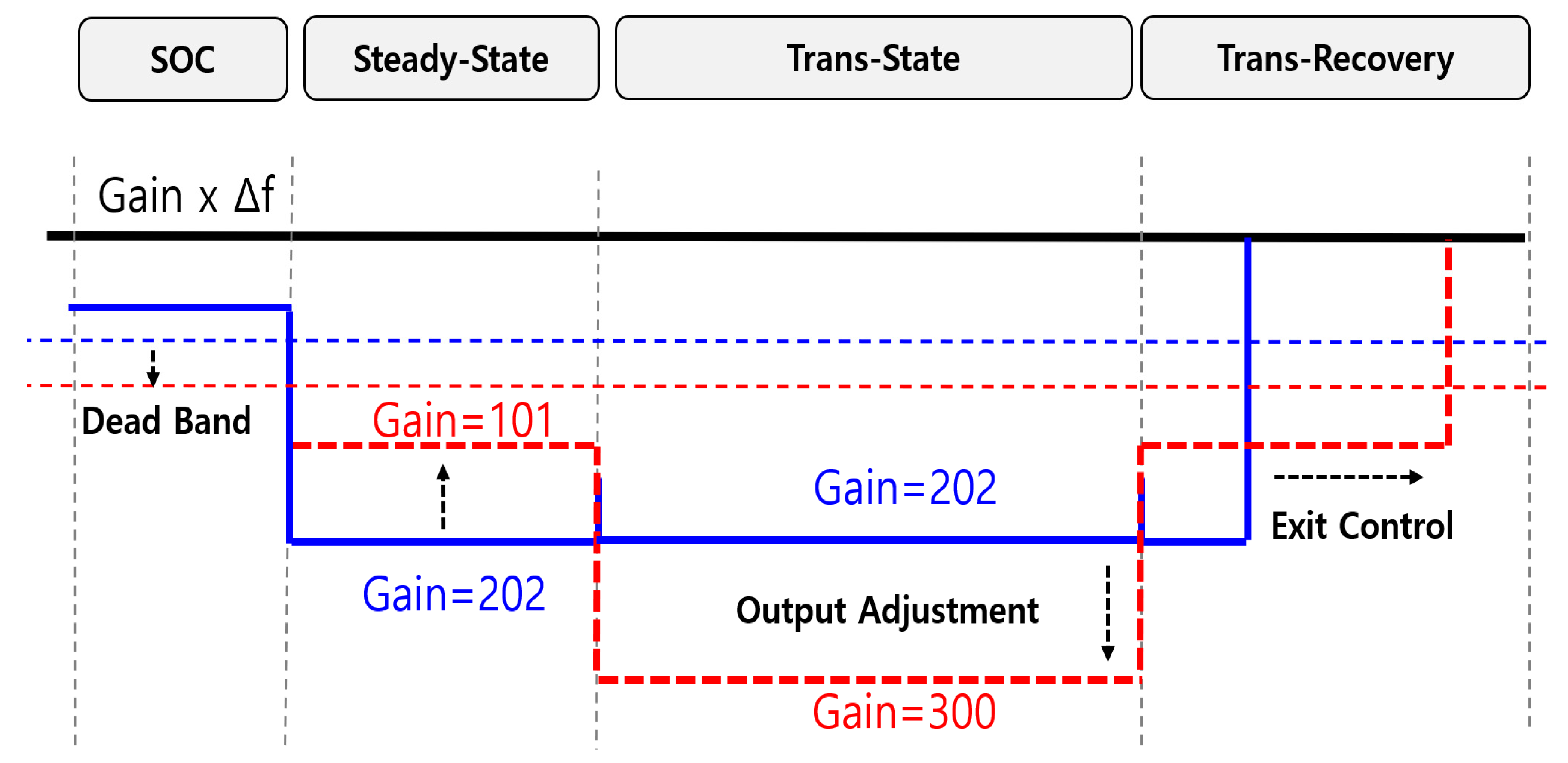
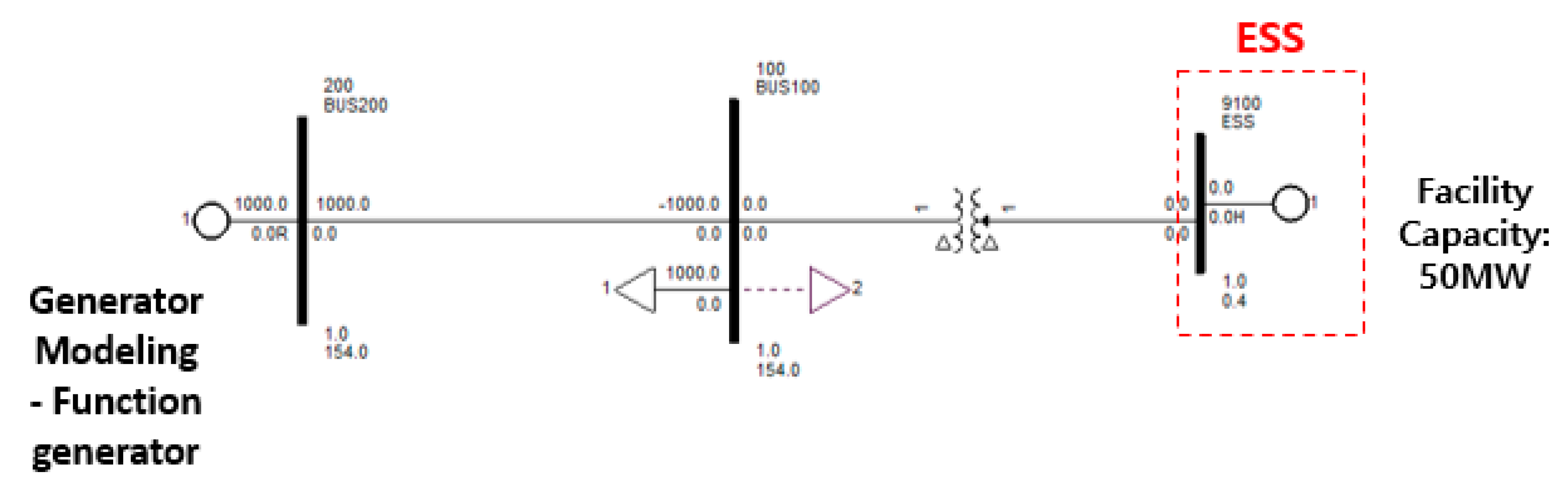
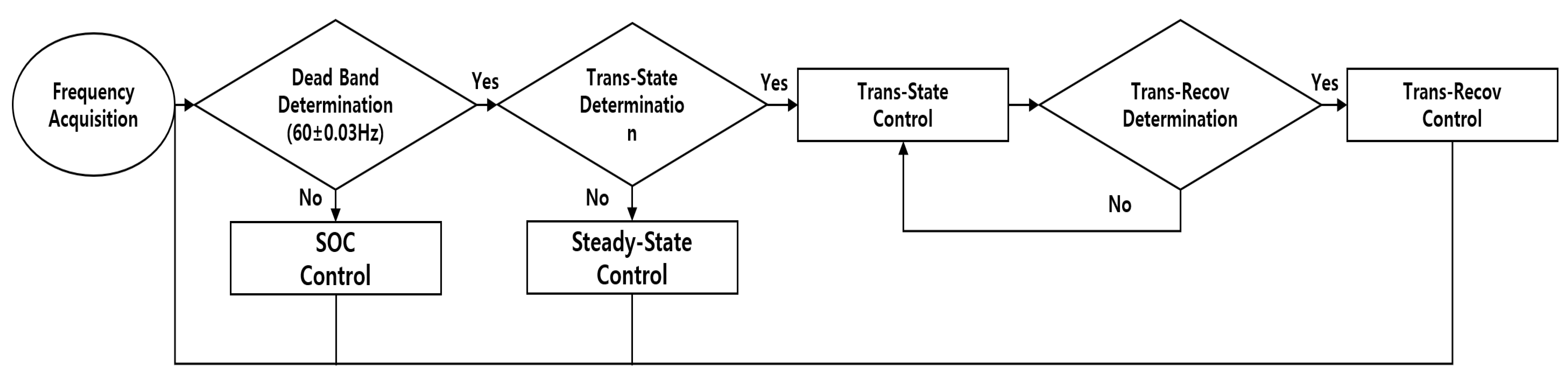
2.3. ESS Modeling
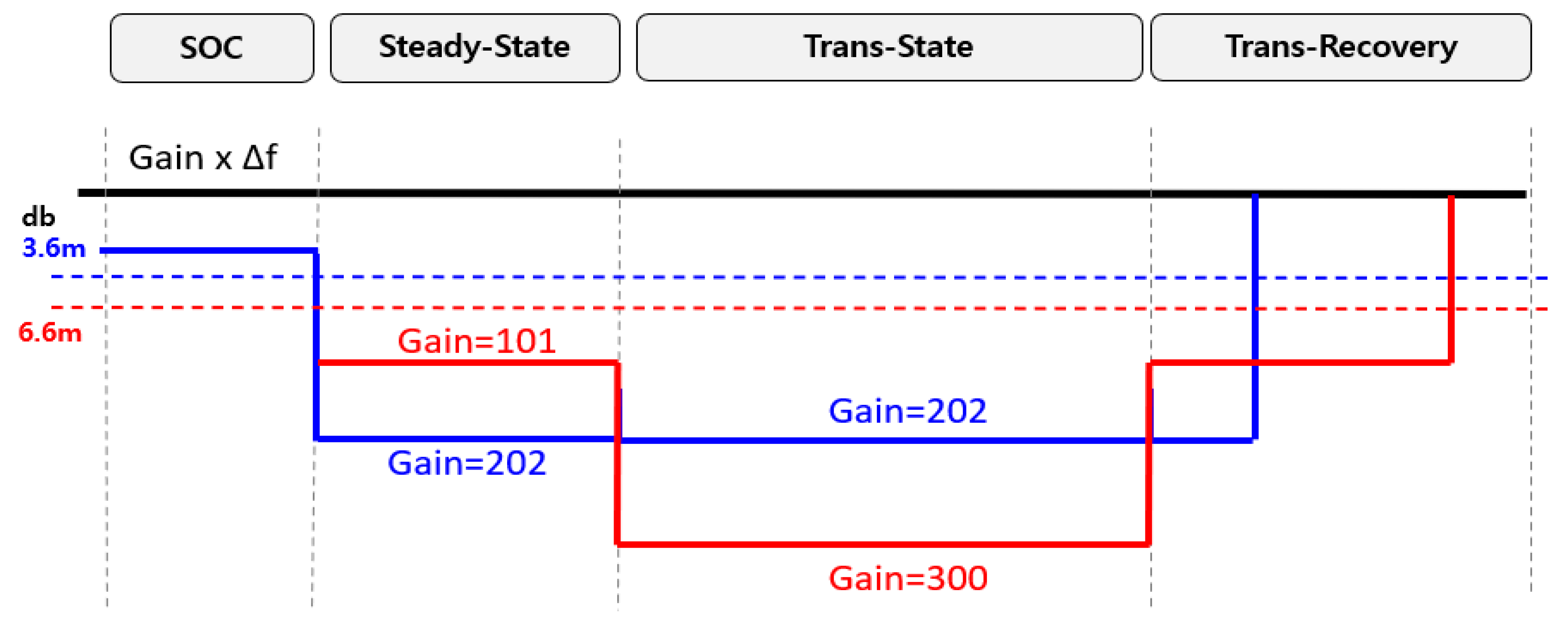
- SOC control: control within the dead band, output, or nonoutput, according to the droop speed.
- Steady-state control: when the dead band is reached, the frequency change rate is limited to the set value, and the output is determined by the droop speed.
- Trans-state control: control when the frequency change rate exceeds the set value after exceeding the dead band; maximum output with constant system applied.
- Trans-recovery control: in the transient state, the frequency increases, and when the increased time exceeds the set value, control, and output, according to the speed adjustment rate.
2.4. Renewable Energy Modeling
- Modeling elements: control mode (power factor, voltage), power factor, reactive power supply range.
- Control mode modeling: modellable through WOD settings in PSS/E generators.
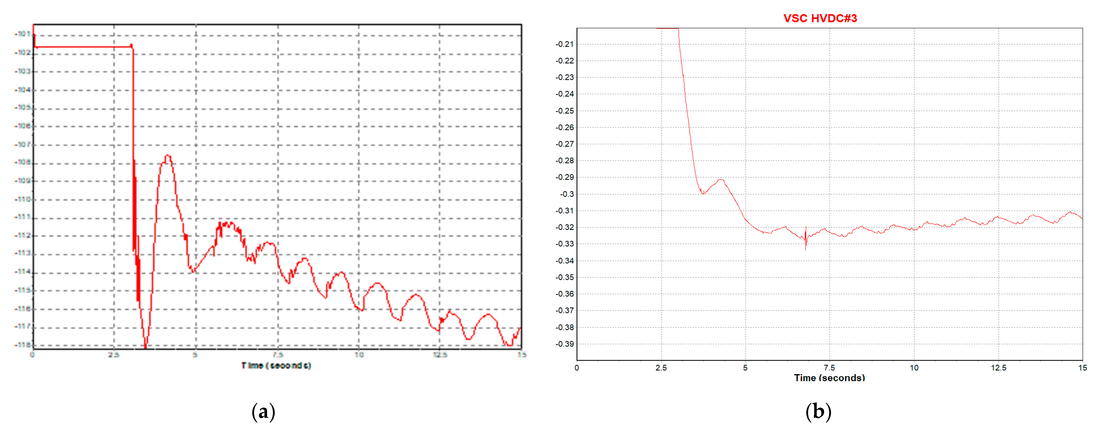
2.5. HVDC#3 Performance Analysis
3. Case Study
3.1. Scenario A
3.2. Scenario B
3.3. Scenario C
- Dead band: ±0.066 Hz;
- RoCoF for trans-state: 0.2 Hz/s;
- Droop speed (trans-recovery): 0.66%;
- System H for trans-state (ESS output).
- ESS#1: steady-state/exit control section quick response, fast exit control.
- ESS#2: fast response in case of transient response, accurate exit control.
- Maintenance, wide dead band.
4. Conclusions
Author Contributions
Funding
Informed Consent Statement
Acknowledgments
Conflicts of Interest
Abbreviations
| ESS | energy storage system |
| PV | photovoltaics |
| RE | renewable energy |
| Gridpl | power system |
| PSH | pumped storage hydroelectricity |
| HVDC | high voltage direct current |
| FFR | fast frequency response |
| PFR | primary frequency response |
| RoCoF | rate of change of frequency |
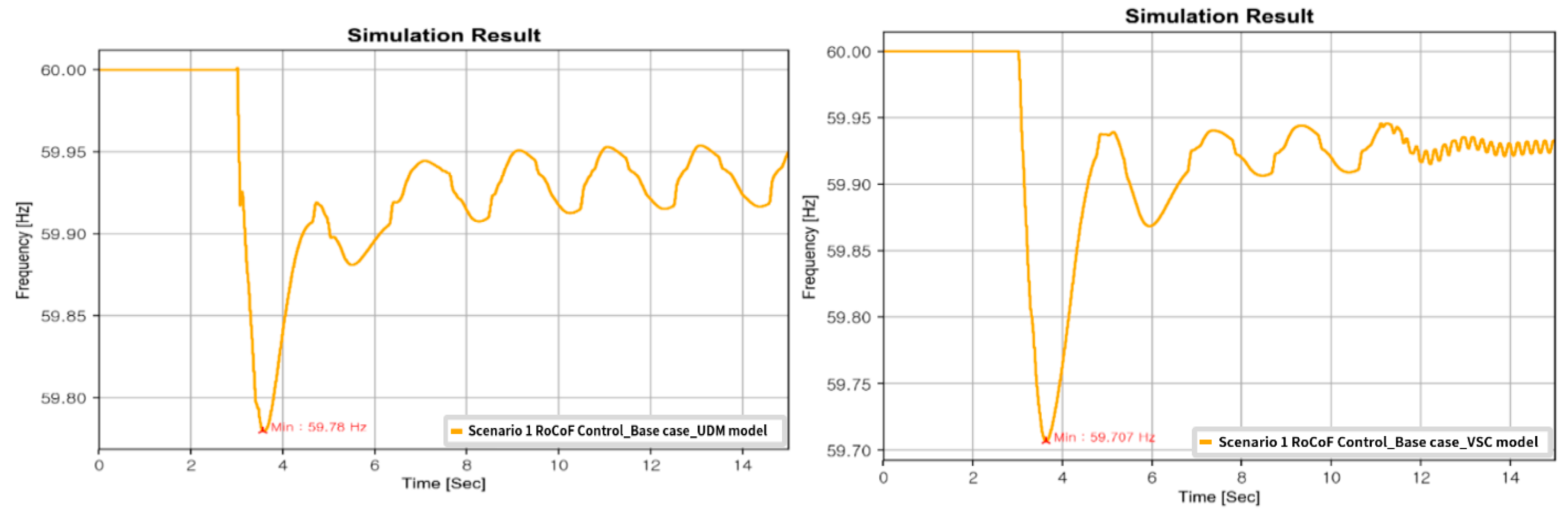
| UDM | user defined model |
| VSC | voltage source convertor |
| Trans-state | transient state |
| Steady-state | stationary state/steady state |
| Trans-recovery | transient recovery state |
| SOC | state of charge |
| WECC | western electricity coordinating council |
| Trip | generator trip |
| Fault | three-phase short circuit |
Appendix A
Appendix B
- (1)
- Renewable energy.

- (2)
- HVDC.

- (3)
- Energy storage system(s) (ESS).

References
- Ministry of Trade, Industry and Energy. The 9th Basic Plan for Long-Term Electricity Supply and Demand; Ministry of Trade, Industry and Energy: Sejong City, Korea, 2020.
- ERCOT. Inertia: Basic Concepts and Impacts on the ERCOT Grid; ERCOT: Austin, TX, USA, 2018. [Google Scholar]
- EIRGRID. DS3 Programme Transition Plan; EIRGRID and SONI: Ireland, Dublin, 2018. [Google Scholar]
- ENTSO-E. Nordic Report: Future System Inertia; ENTSO-E: Brussels, Belgium, 2018. [Google Scholar]
- Arévalo, P.; Tostado-Véliz, M.; Jurado, F. A novel methodology for comprehensive planning of battery storage systems. J. Energy Storage 2021, 37, 102456. [Google Scholar] [CrossRef]
- MISO. Renewable Integration Impact Assessment; MISO: Carmel, IN, USA, 2018. [Google Scholar]
- NERC. Fast Frequency Response Concepts and Bulk Power System Reliability Needs; NERC: Atlanta, GA, USA, 2020. [Google Scholar]
- Yoo, G.M. The World of Electricity; The Korean Institute of Electrical Engineers: Seoul, Korea, 2018. [Google Scholar]
- Yoon, M.H.; Lee, J.H.; Song, S.Y.; Yoo, Y.T.; Jand, G.S.; Jung, S.M.; Hwand, S.C. Utilization of Energy Storage System for Frequency Regulation in Large-Scale Transmission System. Energies 2019, 12, 3898. [Google Scholar] [CrossRef] [Green Version]
- Alves, E.F.; Mota, D.S.; Tedeschi, E. Sizing of Hybrid Energy Storage Systems for Inertial and Primary Frequency Control; Frontiers in Energy Research: Lausanne, Switzerland, 2021. [Google Scholar]
- Kpoto, K.; Sharma, A.M.; Sharma, A. Effect of Energy Storage System in Low Inertia Power System with High Renewable Energy Sources; IEEE: New York, NY, USA, 2019. [Google Scholar]
- MISO. MISO MOD-032 Model Data Requirements & Reporting Procedures; MISO: Carmel, IN, USA, 2015. [Google Scholar]
- Zhao, B.; Wang, X.; Haessing, P. A Novel SoC Feedback Control of ESS for Frequency Regulation of Fractional Frequency Transmission System with Offshore Wind Power; IEEE: New York, NY, USA, 2017. [Google Scholar]
- Denholm, P.L.; Sun, Y.; Mai, T.T. An Introduction to Grid Services: Concepts, Technical Requirements, and Provision from Wind; NREL: Golden, CO, USA, 2019.
- SIEMENS. PSS/E Model Library; SIEMENS: Munich, Germany, 2018. [Google Scholar]
- NERC. Modeling Notification: Recommended Practices for Modeling Momentary Cessation; NERC: Atlanta, GA, USA, 2018. [Google Scholar]


| Year | Division | Coal | LNG | RE | PSH | ETC | HVDC | Total |
|---|---|---|---|---|---|---|---|---|
| 2022 | Capacity (MW) | - | 480 | 1996 | - | 106 | 600 | 3182 |
| Ratio (%) | - | 15.1 | 62.7 | - | 3.3 | 18.9 | 100 | |
| 2030 | Capacity (MW) | - | 480 | 4230 | - | 136 | 600 | 5446 |
| Ratio (%) | - | 8.8 | 77.7 | - | 2.5 | 11.0 | 100 | |
| 2034 | Capacity (MW) | - | 480 | 4456 | - | 136 | 600 | 5672 |
| Ratio (%) | - | 8.5 | 78.6 | - | 2.3 | 10.6 | 100 |
| Configuration | |
|---|---|
| Wind | Company Registration Model |
| PV | 2nd Generic Models |
| HVDC No.1,2 | Company Registration Model |
| HVDC No.3 | VSC and frequency controller Model |
| On-Shore | 2022 year Database |
| Scenario | Load (MW) | Renewable | HVDC No.1,2 | Scheduled Generator | ||
|---|---|---|---|---|---|---|
| Wind (MW) | PV (MW) | Supply (MW) | Transmission (MW) | |||
| 1 | 1059 | 0 | 0 | 400 | 0 | 665 |
| 2 | 874 | 83 | 305 | 230 | 0 | 259 |
| 3 | 596 | 128 | 226 | 50 | 50 | 243 |
| 4 | 596 | 148 | 296 | 60 | 160 | 256 |
| 5 | 596 | 129 | 226 | 40 | 70 | 273 |
| Scenario | Load (MW) | Renewable | HVDC No.1,2,3 | Scheduled Generator | ||
|---|---|---|---|---|---|---|
| Wind (MW) | PV (MW) | Supply (MW) | Transmission (MW) | |||
| 1 | 1059 | 0 | 0 | 500 | 0 | 566 |
| 2 | 874 | 84 | 281 | 260 | 0 | 250 |
| 3 | 596 | 129 | 141 | 150 | 50 | 225 |
| 4 | 596 | 129 | 245 | 160 | 160 | 224 |
| 5 | 596 | 129 | 171 | 140 | 70 | 225 |
| Scenario | Load (MW) | Renewable | HVDC No.1,2,3 | Scheduled Generator | ||
|---|---|---|---|---|---|---|
| Wind (MW) | PV (MW) | Supply (MW) | Transmission (MW) | |||
| 1 | 1059 | 0 | 0 | 350 | 100 | 768 |
| 2 | 874 | 200 | 340 | 160 | 100 | 277.6 |
| 3 | 595.7 | 218.6 | 231 | 50 | 150 | 250 |
| 4 | 595.7 | 128.5 | 241.4 | 30 | 170 | 368 |
| 5 | 595.7 | 218.6 | 261.4 | 40 | 170 | 252.4 |
| Scenario 1 | Scenario 2 | Scenario 3 | Scenario 4 | Scenario 5 | |
|---|---|---|---|---|---|
| Characteristic | Non Renewable HVDC No.1,2 Supply | Much Renewable HVDC No.1,2 Supply | Middle Renewable HVDC No.1,2 Circulation | Few Renewable HVDC No.1,2 Circulation | Few Renewable HVDC No.1,2 Circulation |
| Scenario | Base Case (0.33%) | Droop Speed | ||
|---|---|---|---|---|
| 0.2% | 0.3% | 0.5% | ||
| 1 | 59.75 (59.64) | 59.76 (59.64) | 59.76 (59.64) | 59.73 (59.64) |
| 2 | 59.69 (59.42) | 59.70 (59.43) | 59.69 (59.42) | 59.67 (59.41) |
| 3 | 59.81 (59.56) | 59.82 (59.57) | 59.81 (59.57) | 59.81 (59.57) |
| 4 | 59.87 (58.99) | 59.89 (59.19) | 59.87 (59.74) | 59.85 (59.61) |
| 5 | 59.79 (59.50) | 59.80 (59.50) | 59.79 (59.50) | 59.76 (59.50) |
| Scenario | Base Case | RoCoF | Droop Speed | System H | |||
|---|---|---|---|---|---|---|---|
| 0.05 | 0.1 | 0.5 | 1.0 | 200 | 300 | ||
| 1 | 59.71 (59.62) | 59.71 (59.62) | 59.71 (59.62) | 59.71 (59.62) | 59.71 (59.63) | 59.75 (59.64) | 59.76 (59.64) |
| 2 | 59.64 (59.42) | 59.64 (59.42) | 59.64 (59.42) | 59.63 (59.42) | 59.63 (59.41) | 59.68 (59.42) | 59.70 (59.42) |
| 3 | 59.79 (59.57) | 59.79 (59.57) | 59.79 (59.57) | 59.79 (59.56) | 59.79 (59.56) | 59.82 (59.57) | 59.82 (59.57) |
| 4 | 59.84 (59.64) | 59.84 (59.64) | 59.84 (59.64) | 59.84 (59.60) | 59.85 (59.59) | 59.87 (59.64) | 59.88 (59.65) |
| 5 | 59.74 (59.49) | 59.74 (59.49) | 59.74 (59.49) | 59.74 (59.49) | 59.73 (59.49) | 59.77 (59.50) | 59.78 (59.50) |
| Scenario 1 | Scenario 2 | Scenario 3 | Scenario 4 | Scenario 5 | |
|---|---|---|---|---|---|
| Characteristic | Non Renewable HVDC No.1,2 Supply | Much Renewable HVDC No.1,2 Supply | Middle Renewable HVDC No.1,2 Circulation | Few Renewable HVDC No.1,2 Circulation | Middle Renewable HVDC No.1,2 Supply |
| HVDC#3 VSC Model including Frequency Controller (Supply) | |||||
| Scenario | Base Case (0.33%) | Droop Speed | ||
|---|---|---|---|---|
| 0.2% | 0.3% | 0.5% | ||
| 1 | 59.74 (59.58) | 59.75 (59.58) | 59.74 (59.58) | 59.73 (59.58) |
| 2 | 59.71 (59.62) | 59.72 (59.61) | 59.71 (59.62) | 59.69 (59.63) |
| 3 | 59.84 (59.66) | 59.85 (59.65) | 59.85 (59.66) | 59.82 (59.67) |
| 4 | 59.81 (59.59) | 59.83 (59.58) | 59.81 (59.58) | 59.81 (59.59) |
| 5 | 59.69 (59.78) | 59.70 (59.78) | 59.69 (59.78) | 59.67 (59.78) |
| Scenario | Base Case | RoCoF | Droop Speed | System H | |||
|---|---|---|---|---|---|---|---|
| 0.05 | 0.1 | 0.5 | 1.0 | 200 | 300 | ||
| 1 | 59.71 (59.57) | 59.71 (59.57) | 59.71 (59.57) | 59.71 (59.57) | 59.71 (59.57) | 59.73 (59.58) | 59.75 (59.58) |
| 2 | 59.66 (59.65) | 59.66 (59.65) | 59.66 (59.65) | 59.66 (59.65) | 59.66 (59.65) | 59.70 (59.62) | 59.71 (59.61) |
| 3 | 59.80 (59.66) | 59.80 (59.66) | 59.80 (59.66) | 59.80 (59.66) | 59.80 (59.66) | 59.83 (59.67) | 59.85 (59.65) |
| 4 | 59.79 (59.57) | 59.79 (59.57) | 59.79 (59.57) | 59.79 (59.57) | 59.79 (59.57) | 59.81 (59.59) | 59.82 (59.58) |
| 5 | 59.63 (59.78) | 59.63 (59.78) | 59.63 (59.78) | 59.63 (59.78) | 59.63 (59.78) | 59.68 (59.78) | 59.69 (59.78) |
| Scenario 1 | Scenario 2 | Scenario 3 | Scenario 4 | Scenario 5 | |
|---|---|---|---|---|---|
| Characteristic | Non Renewable HVDC No.1,2 Supply | Much Renewable HVDC No.1,2 Supply | Middle Renewable HVDC No.1,2 Circulation | Few Renewable HVDC No.1,2 Circulation | Few Renewable HVDC No.1,2 Circulation |
| HVDC No.3 VSC Model including Frequency Controller (Transmission) | |||||
| Scenario | Base Case (0.33%) | Droop Speed | ||
|---|---|---|---|---|
| 0.2% | 0.3% | 0.5% | ||
| 1 | 59.77 (59.64) | 59.78 (59.64) | 59.77 (59.64) | 59.76 (59.64) |
| 2 | 59.70 (59.45) | 59.71 (59.45) | 59.70 (59.45) | 59.69 (59.45) |
| 3 | 59.84 (59.50) | 59.85 (59.49) | 59.85 (59.49) | 59.82 (59.51) |
| 4 | 59.67 (59.31) | 59.68 (59.31) | 59.67 (59.31) | 59.65 (59.32) |
| 5 | 59.68 (59.36) | 59.70 (59.36) | 59.69 (59.36) | 59.67 (59.36) |
| Scenario | Base Case | RoCoF | Droop Speed | System H | |||
|---|---|---|---|---|---|---|---|
| 0.05 | 0.1 | 0.5 | 1.0 | 200 | 300 | ||
| 1 | 59.74 (59.62) | 59.74 (59.62) | 59.74 (59.62) | 59.74 (59.62) | 59.74 (59.62) | 59.76 (59.64) | 59.78 (59.64) |
| 2 | 59.65 (59.47) | 59.65 (59.47) | 59.65 (59.47) | 59.65 (59.47) | 59.65 (59.46) | 59.70 (59.45) | 59.70 (59.44) |
| 3 | 59.80 (59.51) | 59.80 (59.51) | 59.80 (59.51) | 59.80 (59.52) | 59.80 (59.52) | 59.83 (59.50) | 59.85 (59.49) |
| 4 | 59.61 (59.34) | 59.61 (59.34) | 59.61 (59.34) | 59.61 (59.33) | 59.61 (59.33) | 59.66 (59.31) | 59.67 (59.31) |
| 5 | 59.63 (59.36) | 59.63 (59.36) | 59.63 (59.36) | 59.62 (59.36) | 59.62 (59.36) | 59.68 (59.36) | 59.69 (59.36) |
| Scenario 1 | Scenario 2 | Scenario 3 | Scenario 4 | Scenario 5 | |
|---|---|---|---|---|---|
| Scenario B | 59.74 (59.71) | 59.71 (59.66) | 59.84 (59.80) | 59.82 (59.79) | 59.69 (59.63) |
| Scenario C | 59.77 (59.74) | 59.70 (59.65) | 59.82 (59.80) | 59.67 (59.61) | 59.68 (59.63) |
| Scenario 1 | Scenario 2 | Scenario 3 | Scenario 4 | Scenario 5 | |
|---|---|---|---|---|---|
| Scenario B | 59.58 (59.57) | 59.66 (59.65) | 59.66 (59.66) | 59.57 (59.57) | 59.78 (59.78) |
| Scenario C | 59.64 (59.62) | 59.48 (59.47) | 59.52 (59.51) | 59.34 (59.34) | 59.36 (59.36) |
Publisher’s Note: MDPI stays neutral with regard to jurisdictional claims in published maps and institutional affiliations. |
© 2022 by the authors. Licensee MDPI, Basel, Switzerland. This article is an open access article distributed under the terms and conditions of the Creative Commons Attribution (CC BY) license (https://creativecommons.org/licenses/by/4.0/).
Share and Cite
Jung, J.-Y.; Cho, Y.-S.; Min, J.-H.; Song, H. An Operation Strategy of ESS for Enhancing the Frequency Stability of the Inverter-Based Jeju Grid. Energies 2022, 15, 3086. https://doi.org/10.3390/en15093086
Jung J-Y, Cho Y-S, Min J-H, Song H. An Operation Strategy of ESS for Enhancing the Frequency Stability of the Inverter-Based Jeju Grid. Energies. 2022; 15(9):3086. https://doi.org/10.3390/en15093086
Chicago/Turabian StyleJung, Jin-Yong, Yoon-Sung Cho, Jae-Hyun Min, and Hwachang Song. 2022. "An Operation Strategy of ESS for Enhancing the Frequency Stability of the Inverter-Based Jeju Grid" Energies 15, no. 9: 3086. https://doi.org/10.3390/en15093086
APA StyleJung, J.-Y., Cho, Y.-S., Min, J.-H., & Song, H. (2022). An Operation Strategy of ESS for Enhancing the Frequency Stability of the Inverter-Based Jeju Grid. Energies, 15(9), 3086. https://doi.org/10.3390/en15093086