
Performance Optimization of a Ten Check MPPT Algorithm for an Off-Grid Solar Photovoltaic System

 ,
,  ,
,  and
and 
Abstract
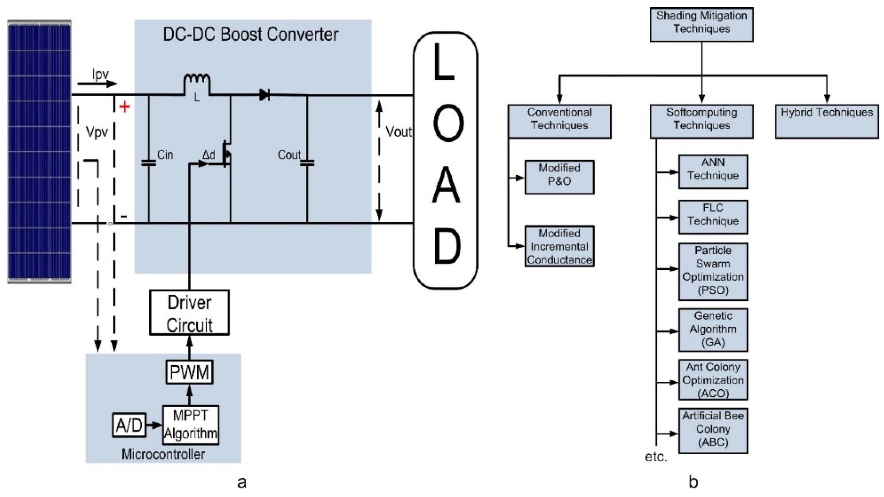
:1. Introduction
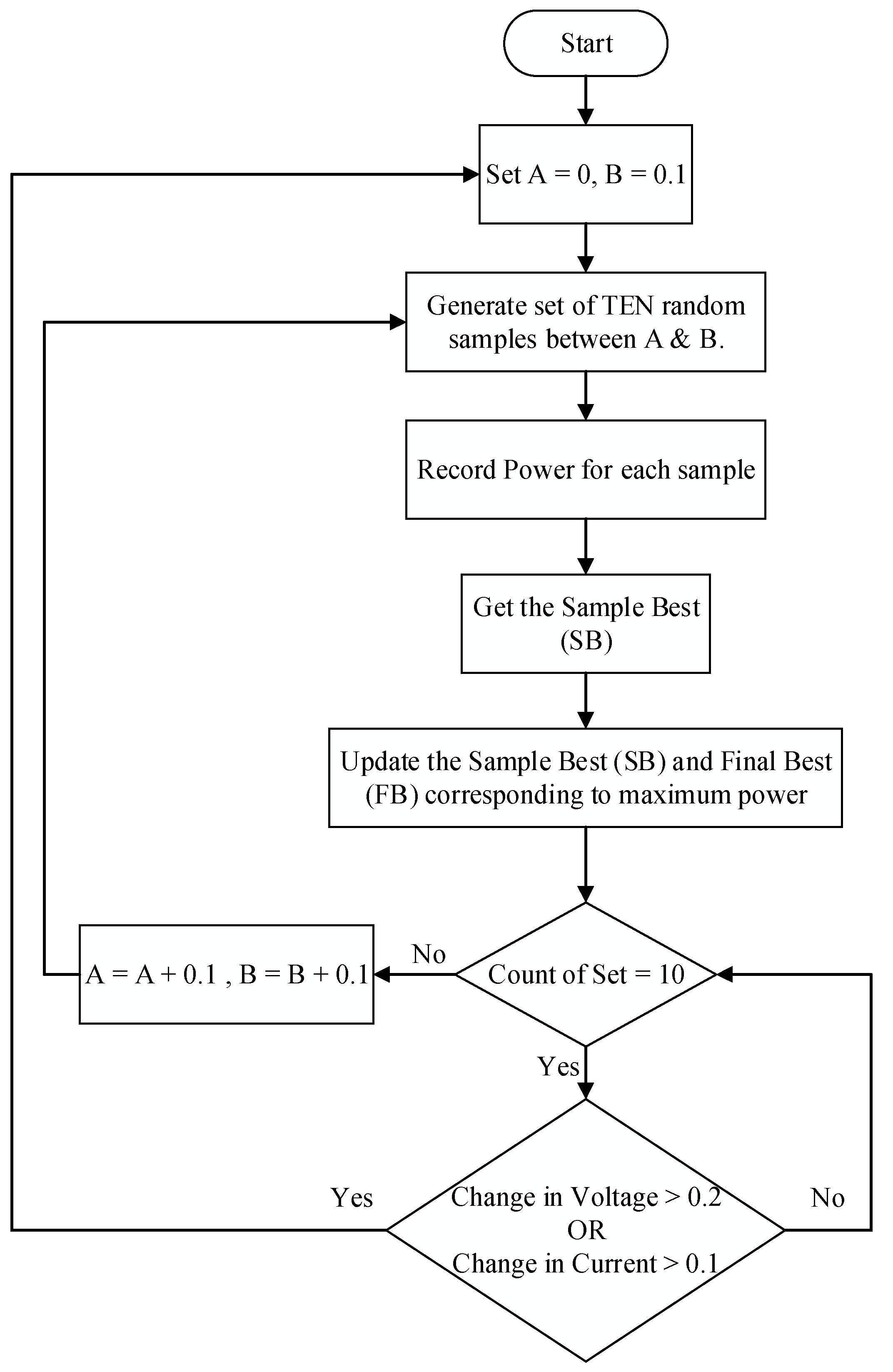
2. Ten Check Algorithm
2.1. SWOT Analysis for the TCA Algorithm
2.2. Problem Statement
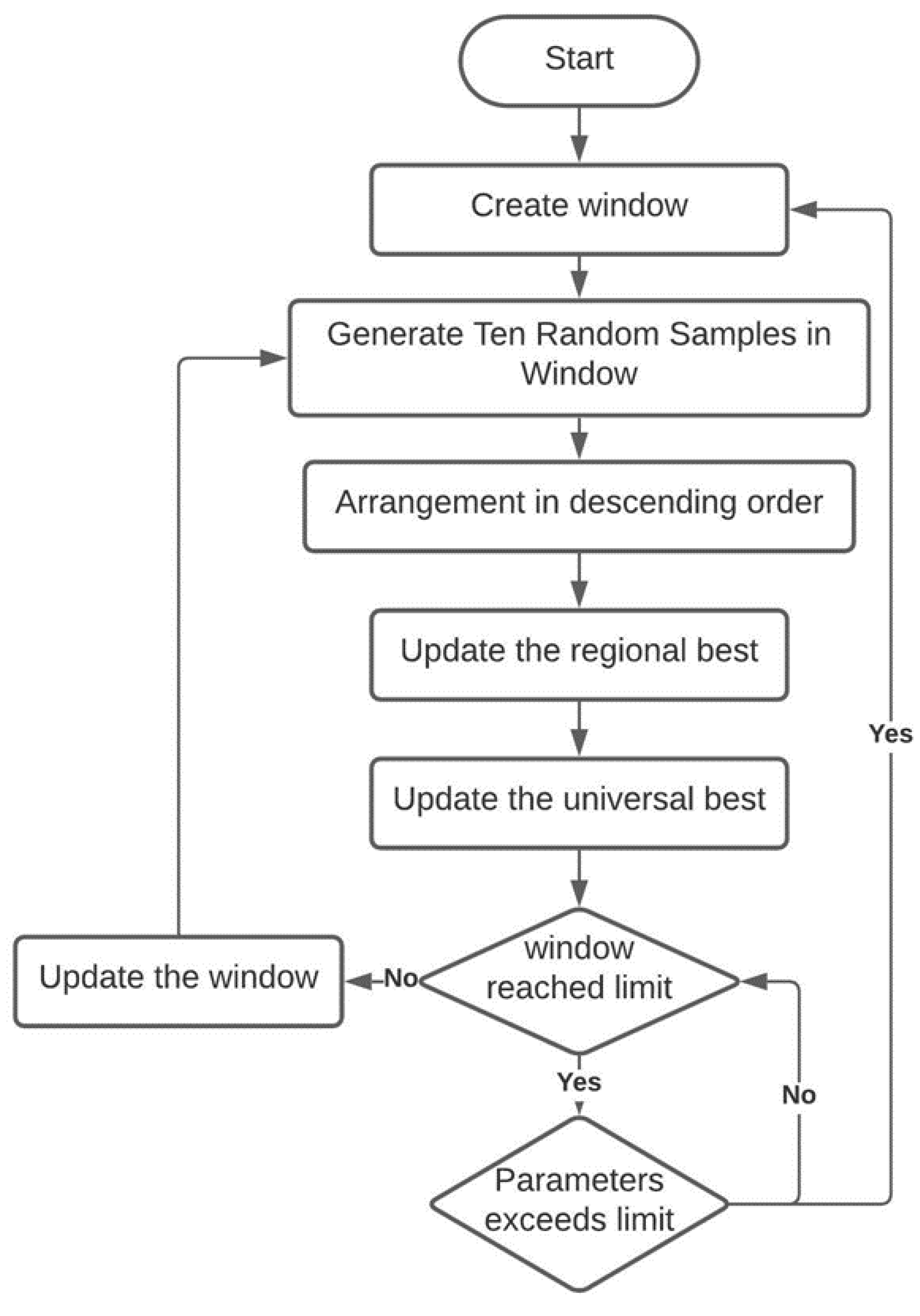
3. Optimized TCA
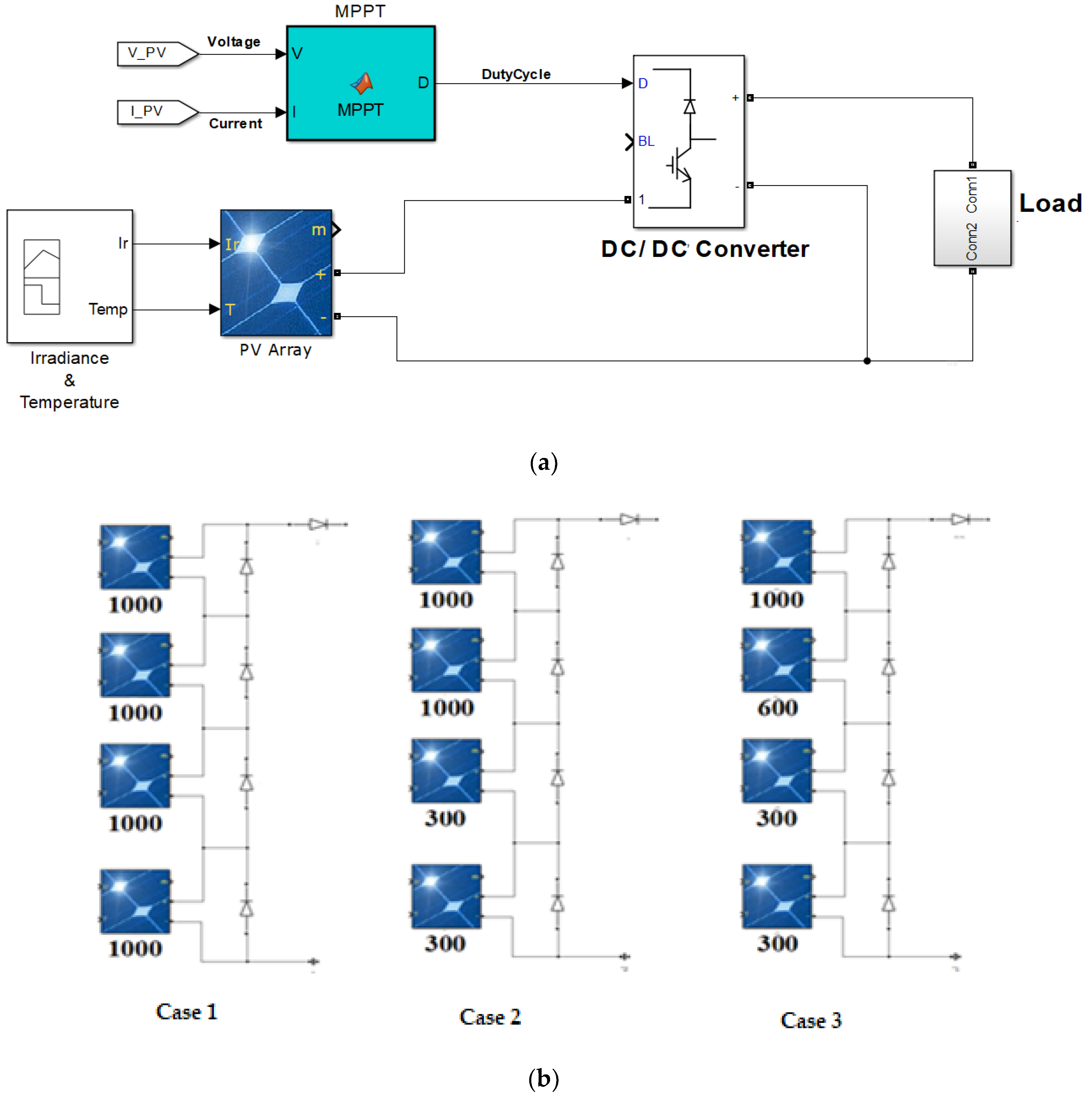
4. Results and Discussion
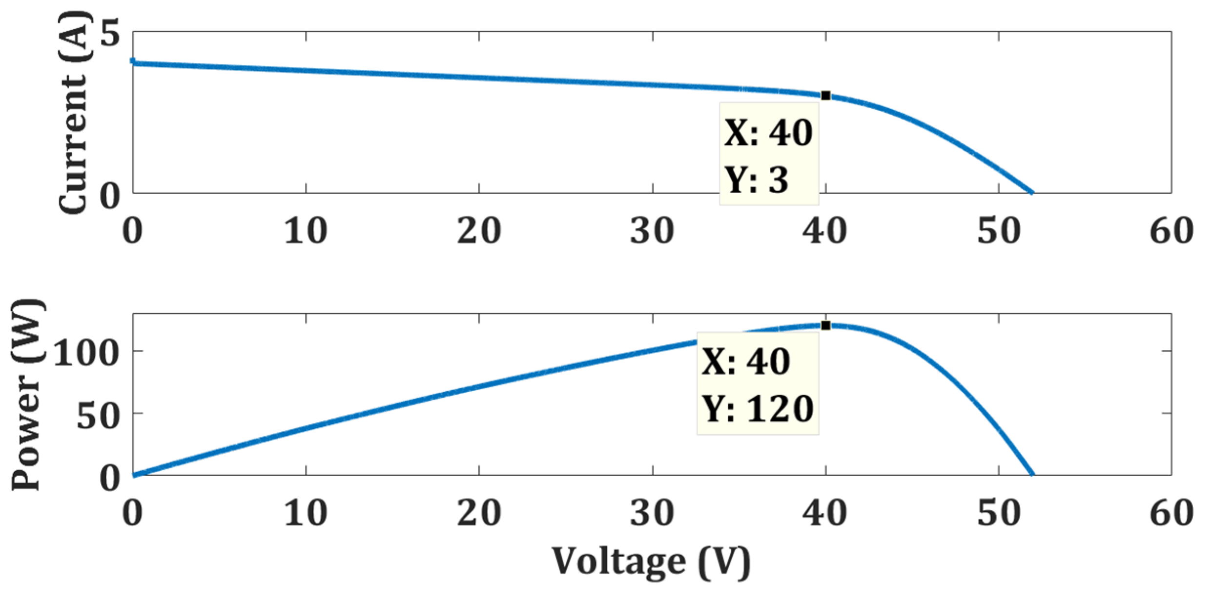
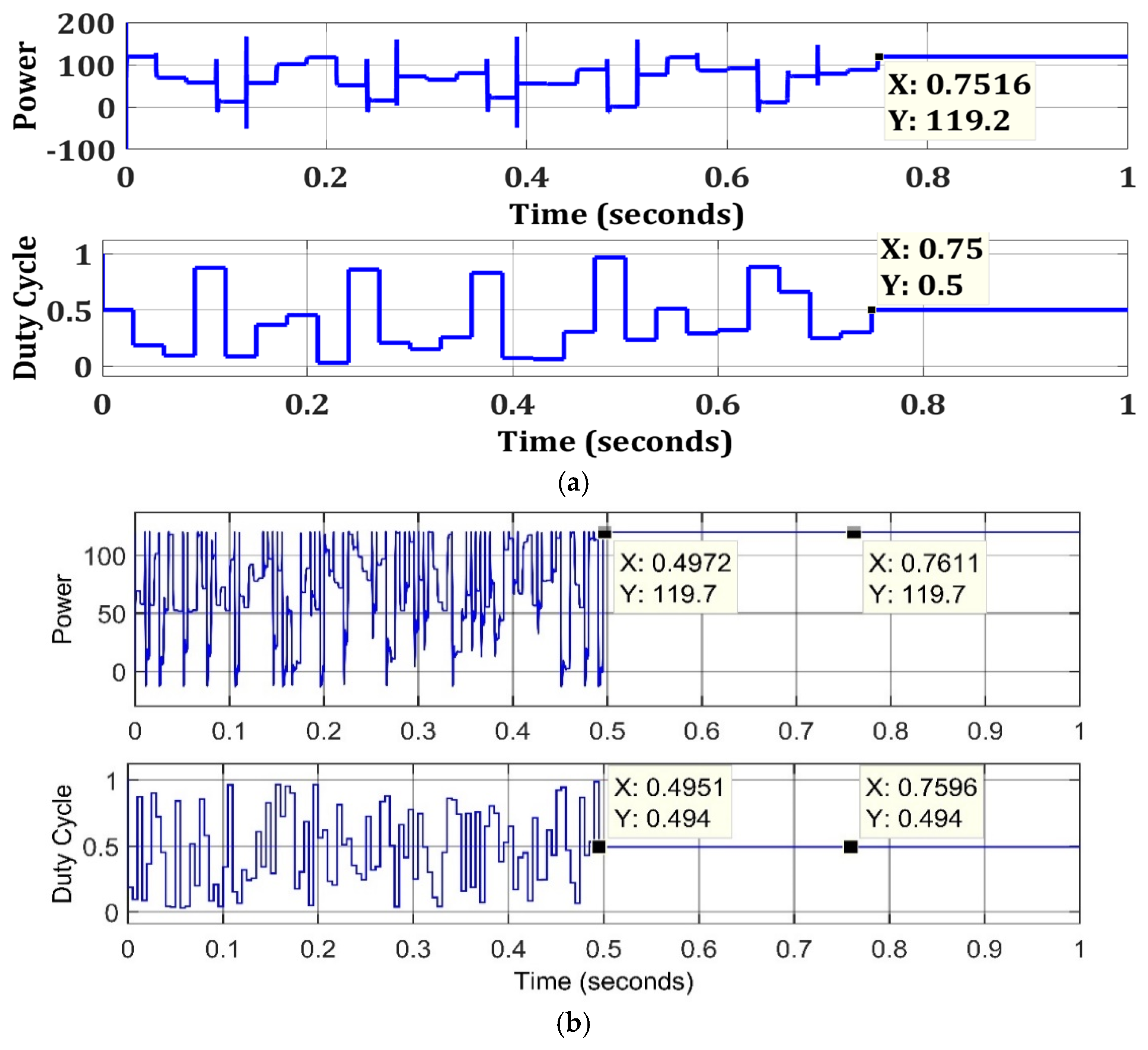
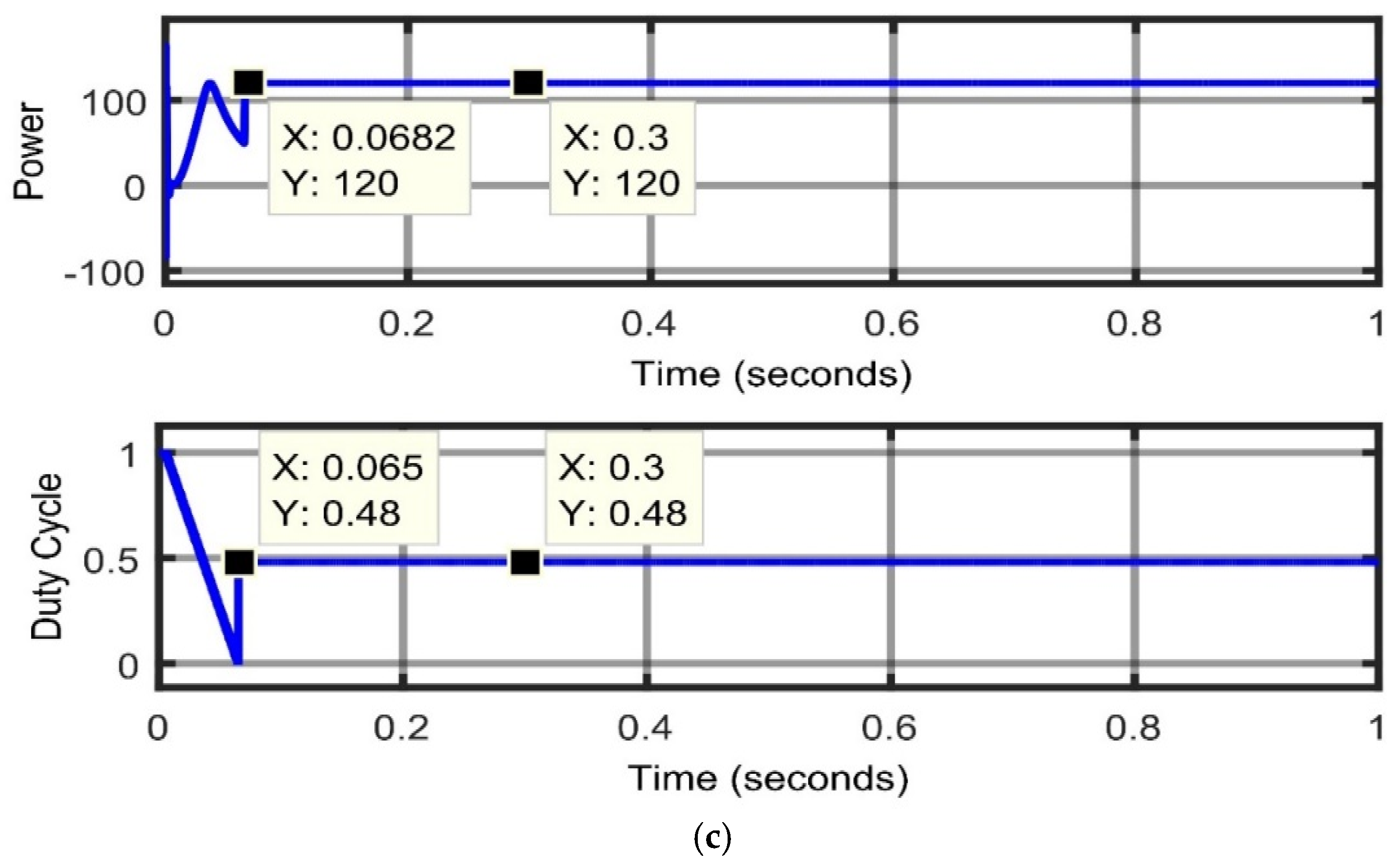
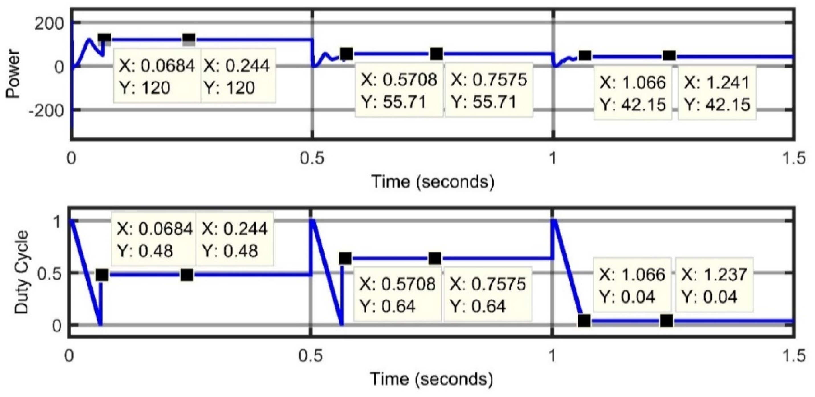
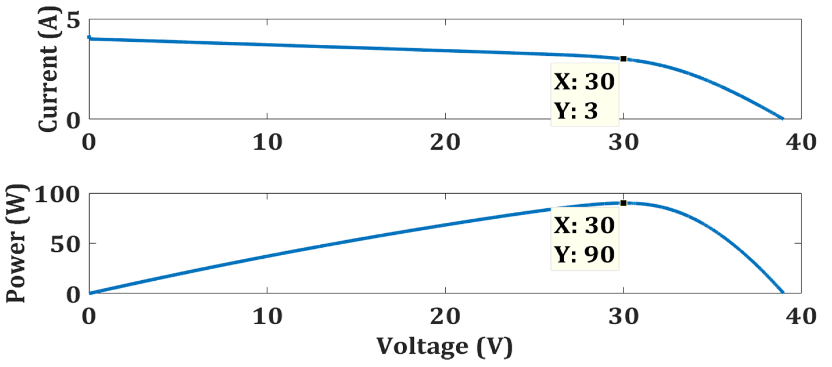
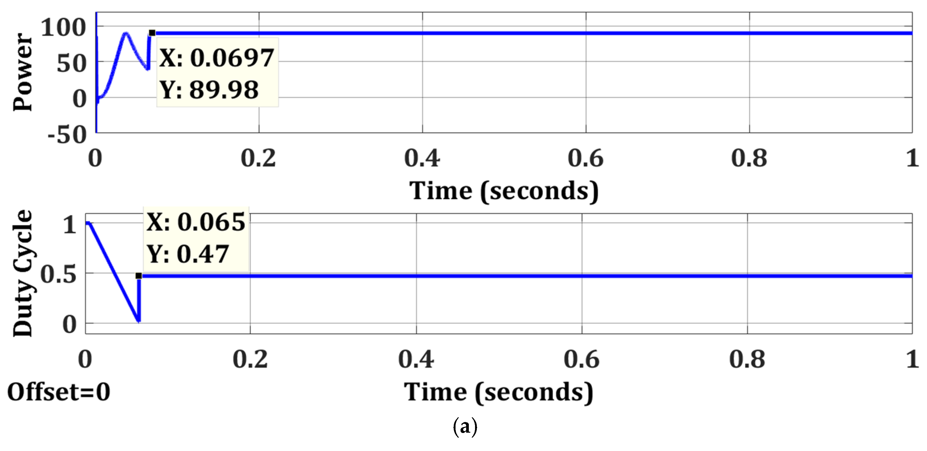
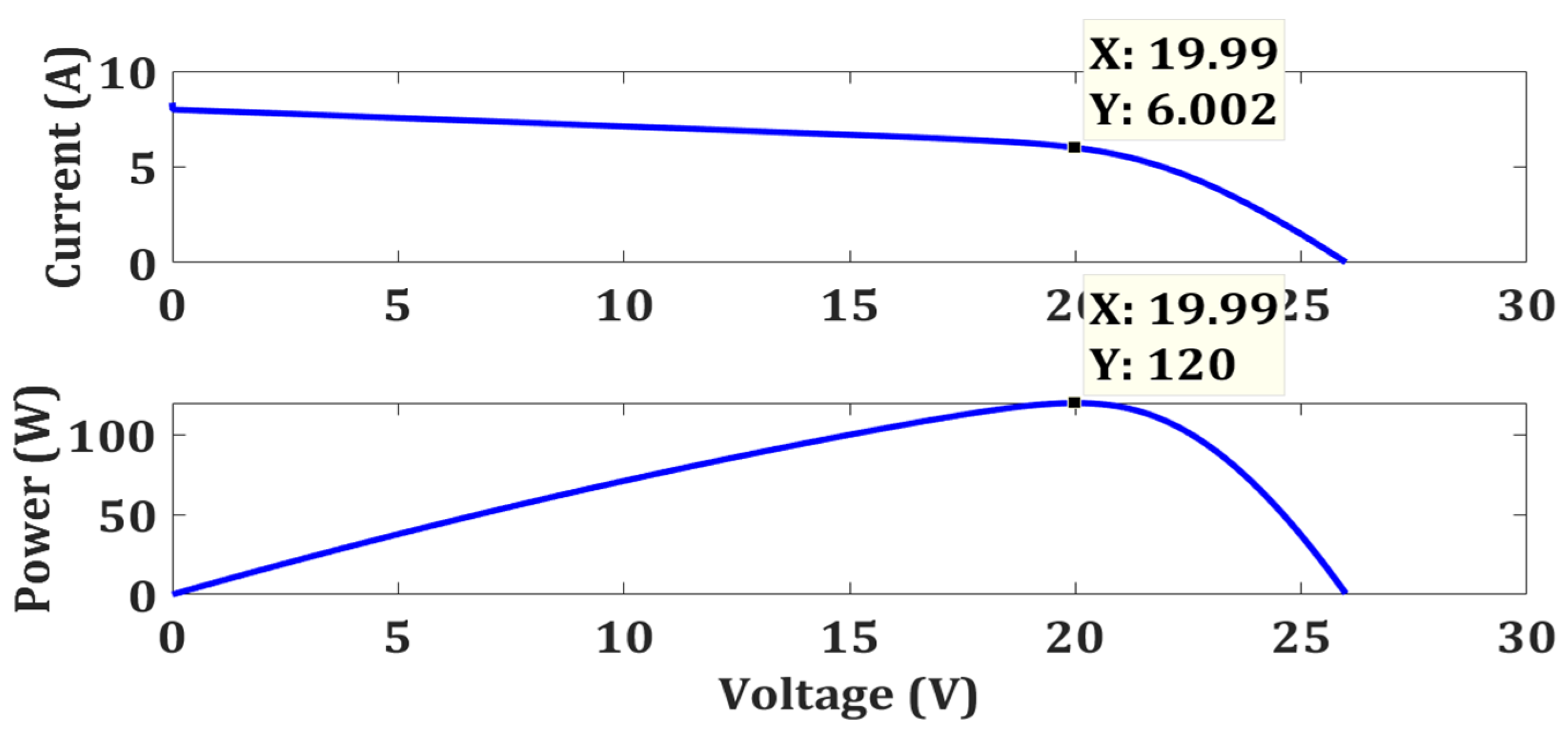
4.1. Uniform Weather Condition
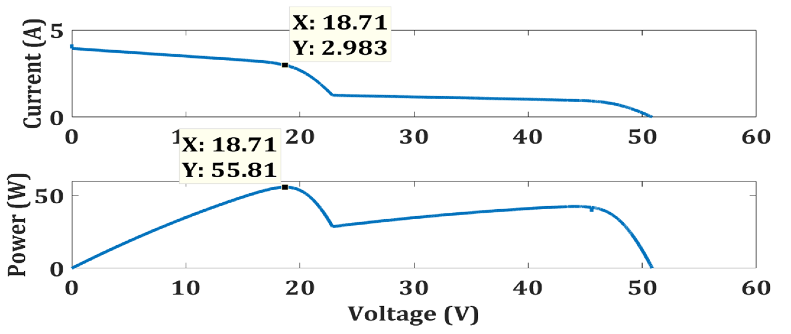
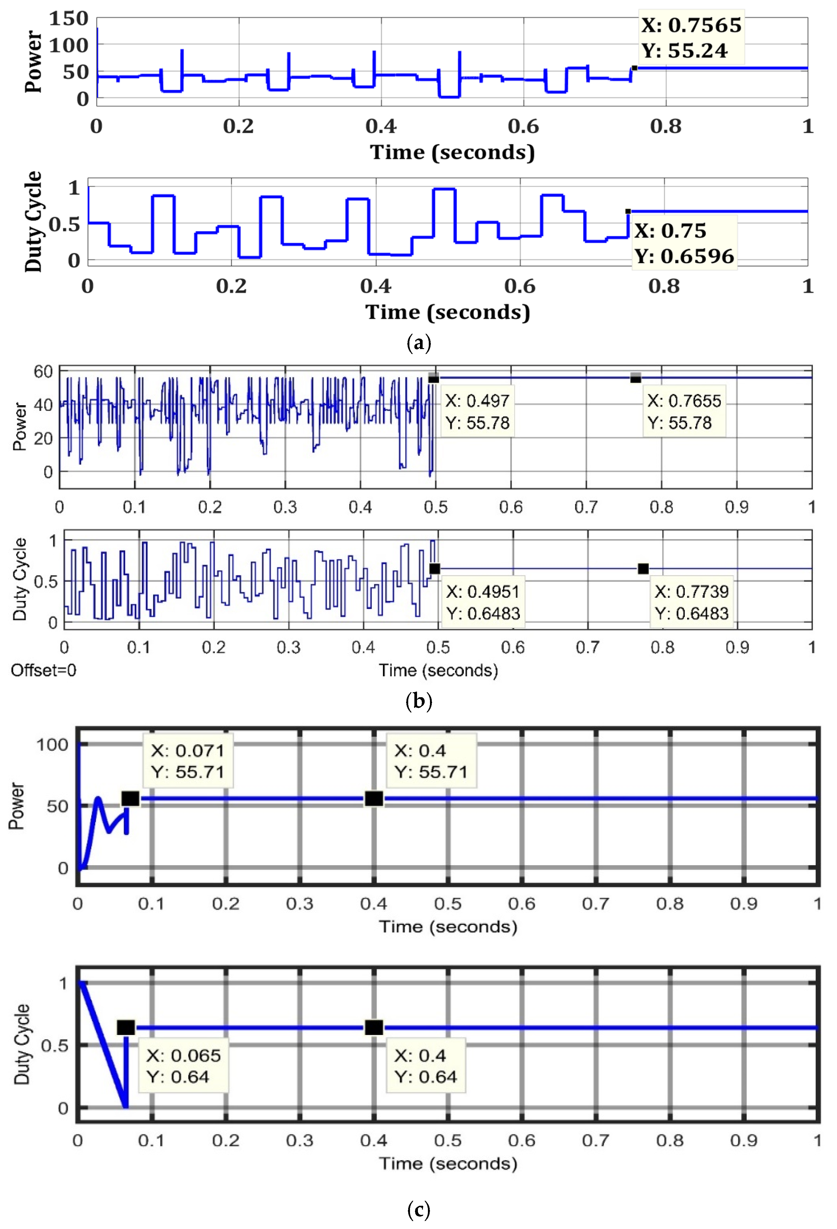
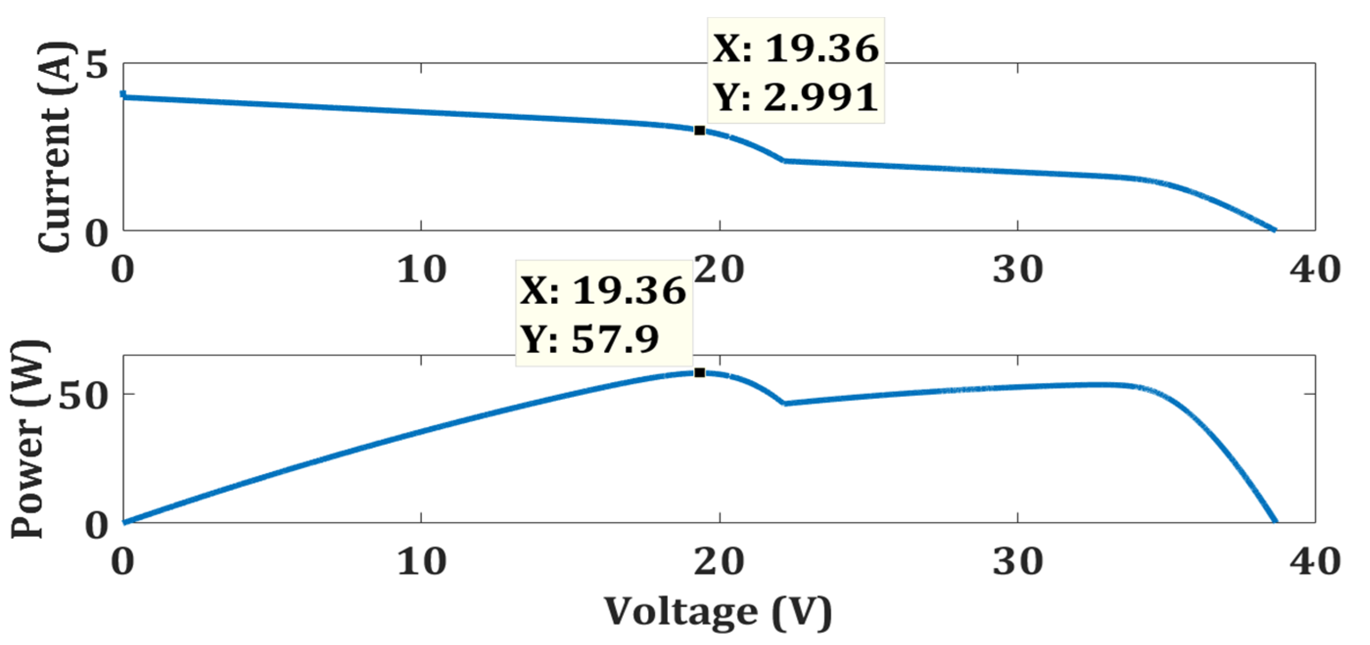
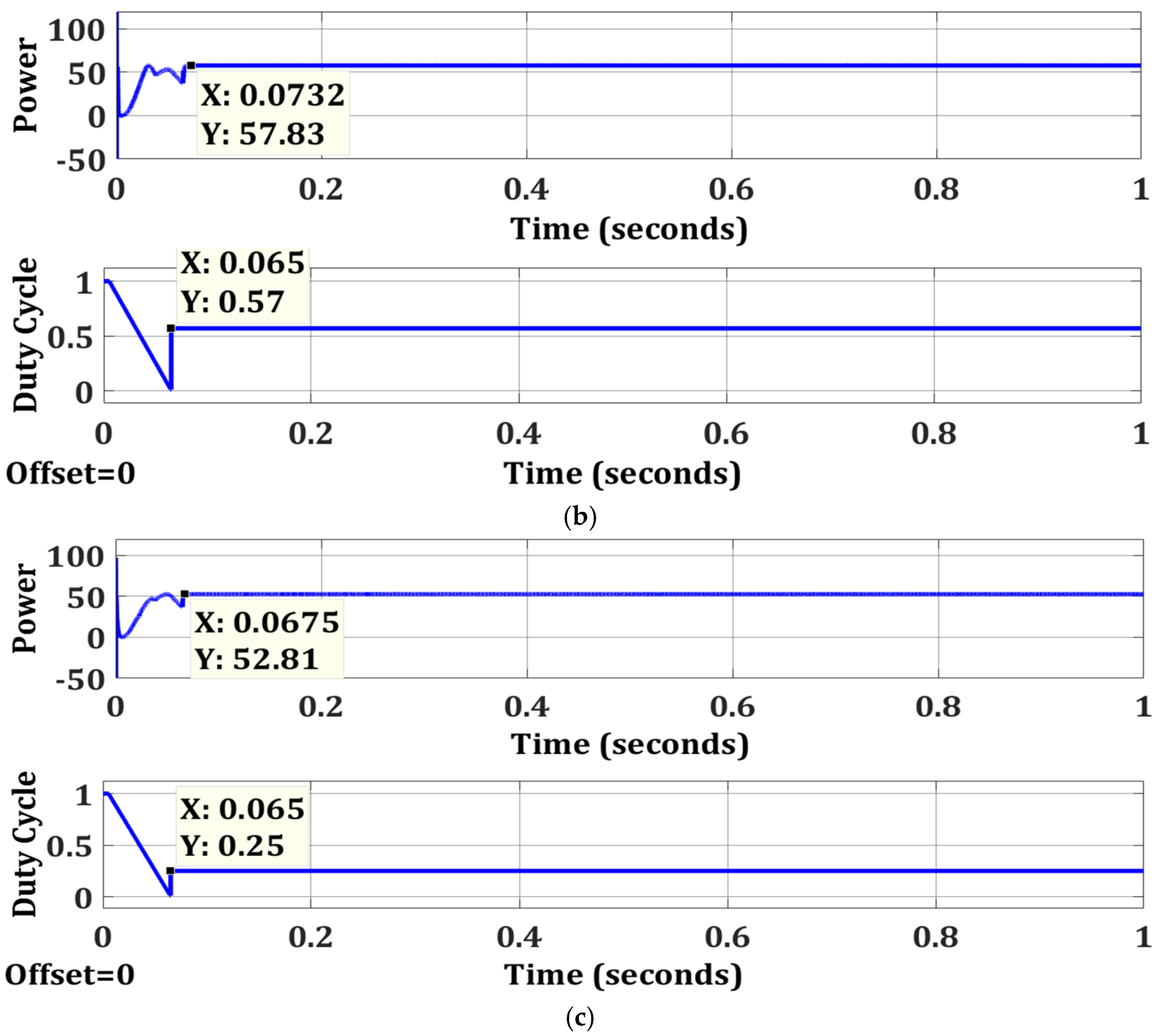
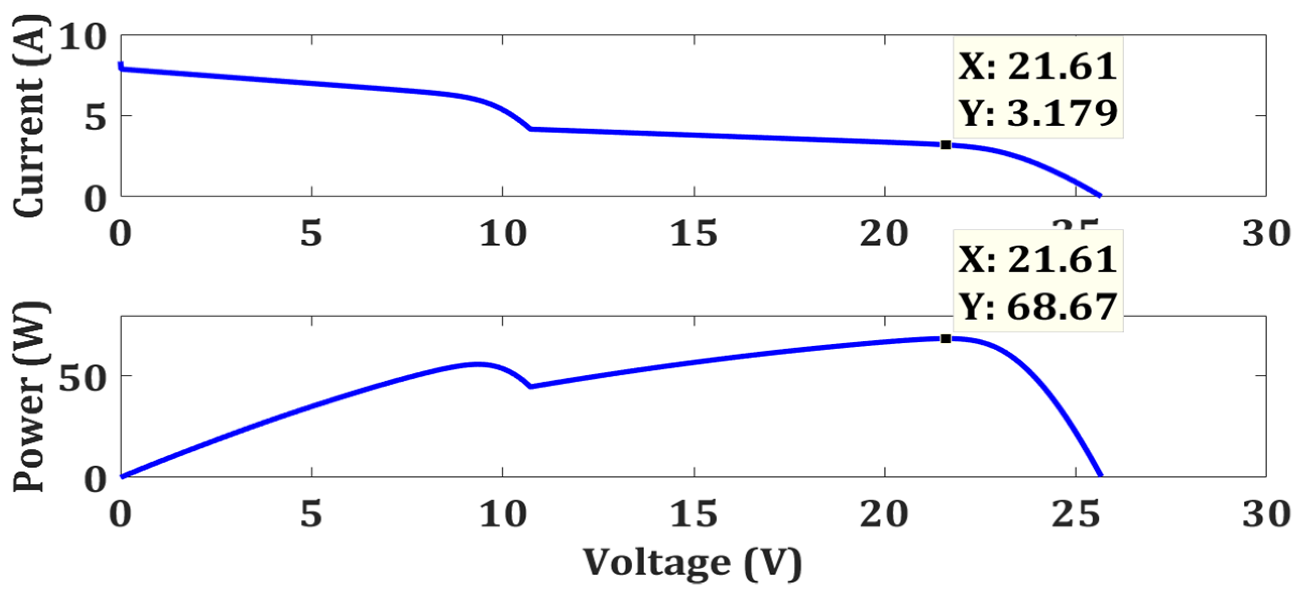
4.2. Weak Partial Shading
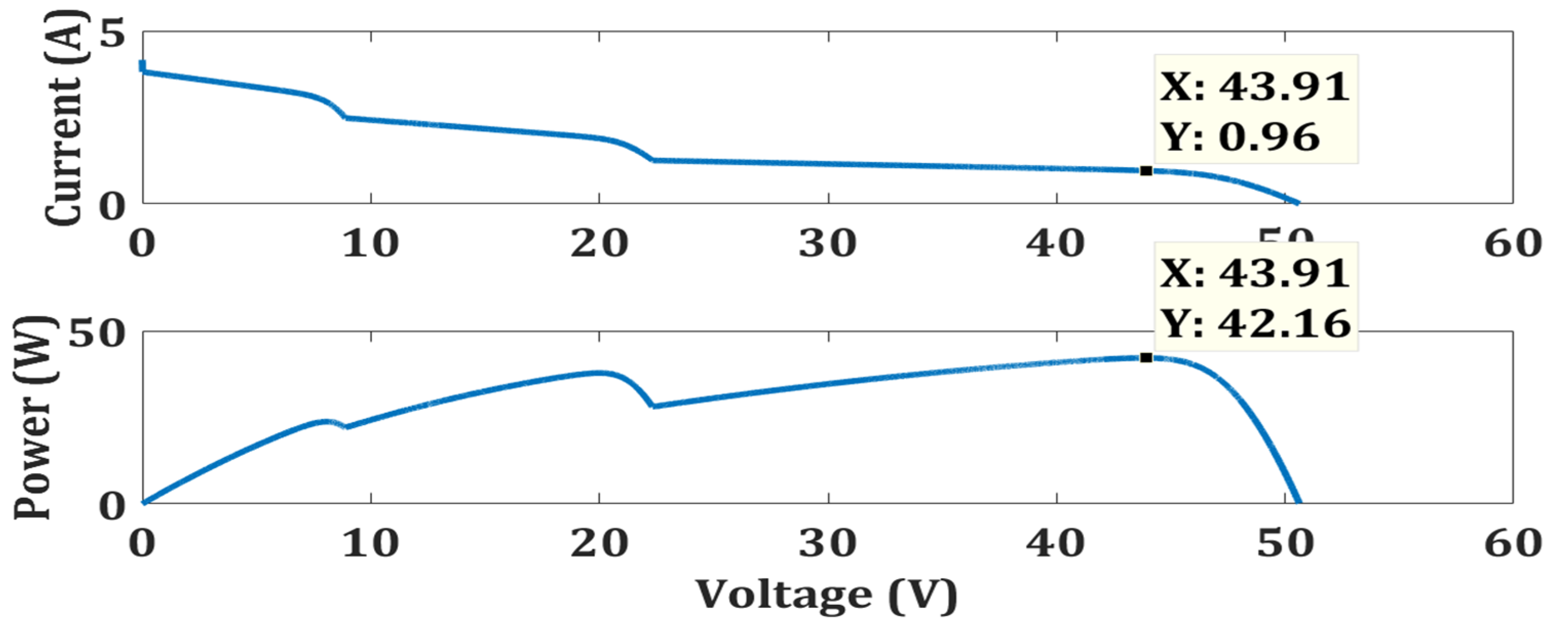
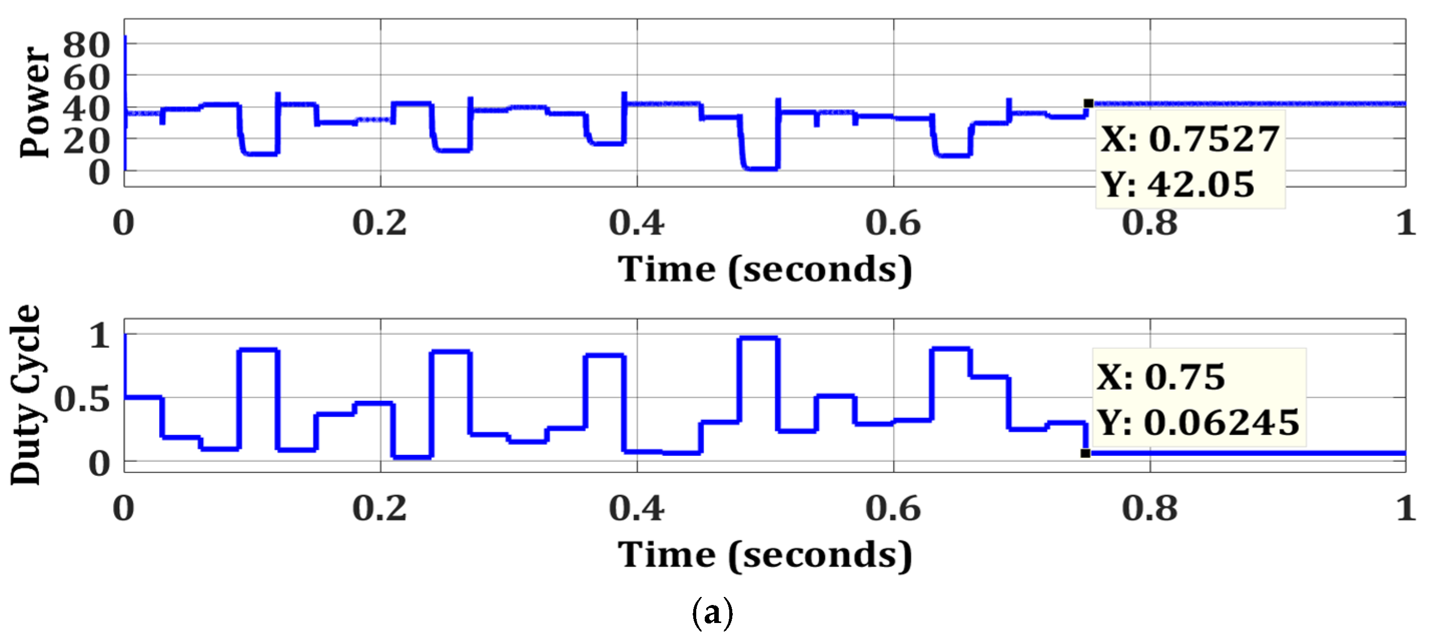
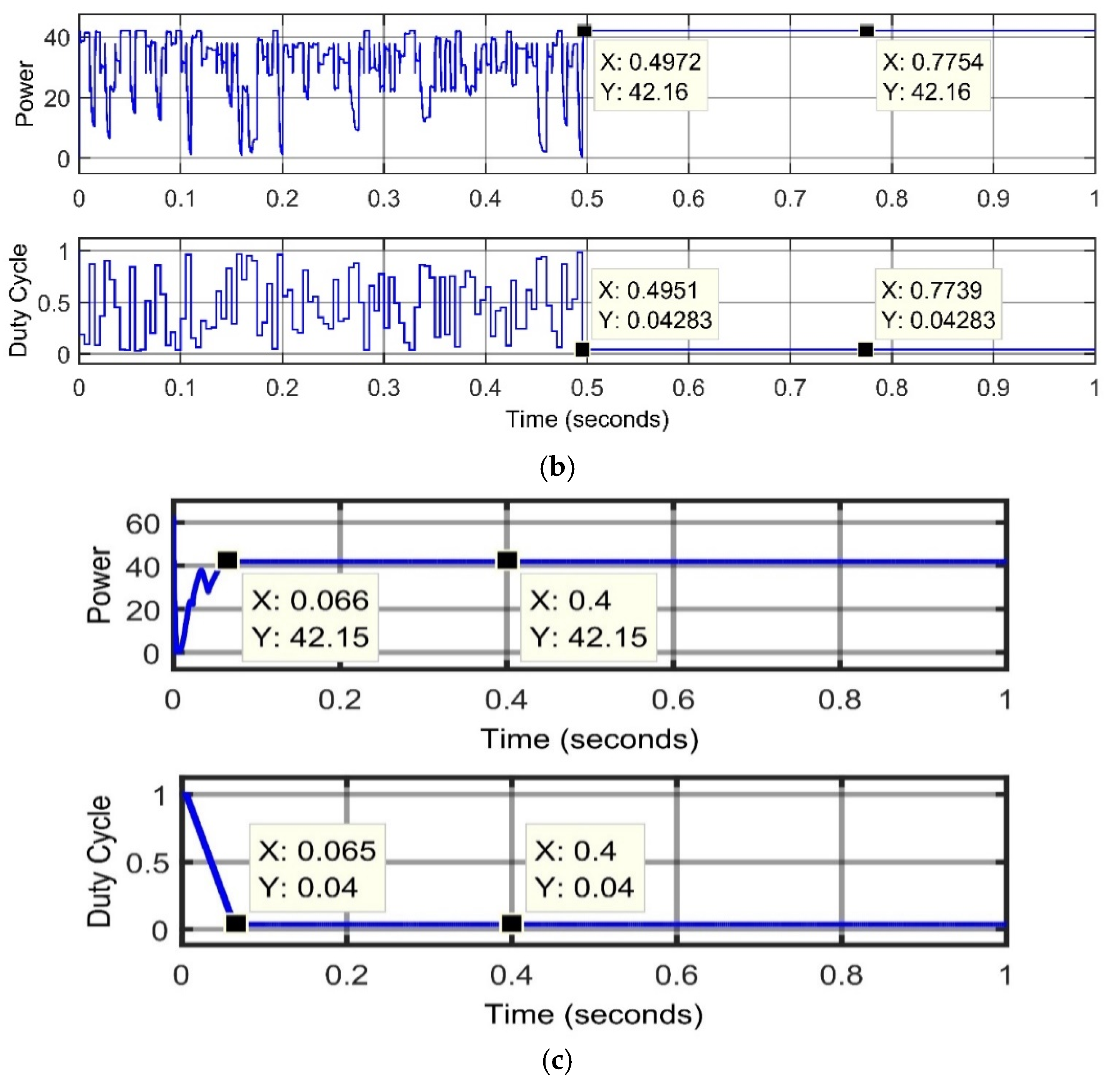
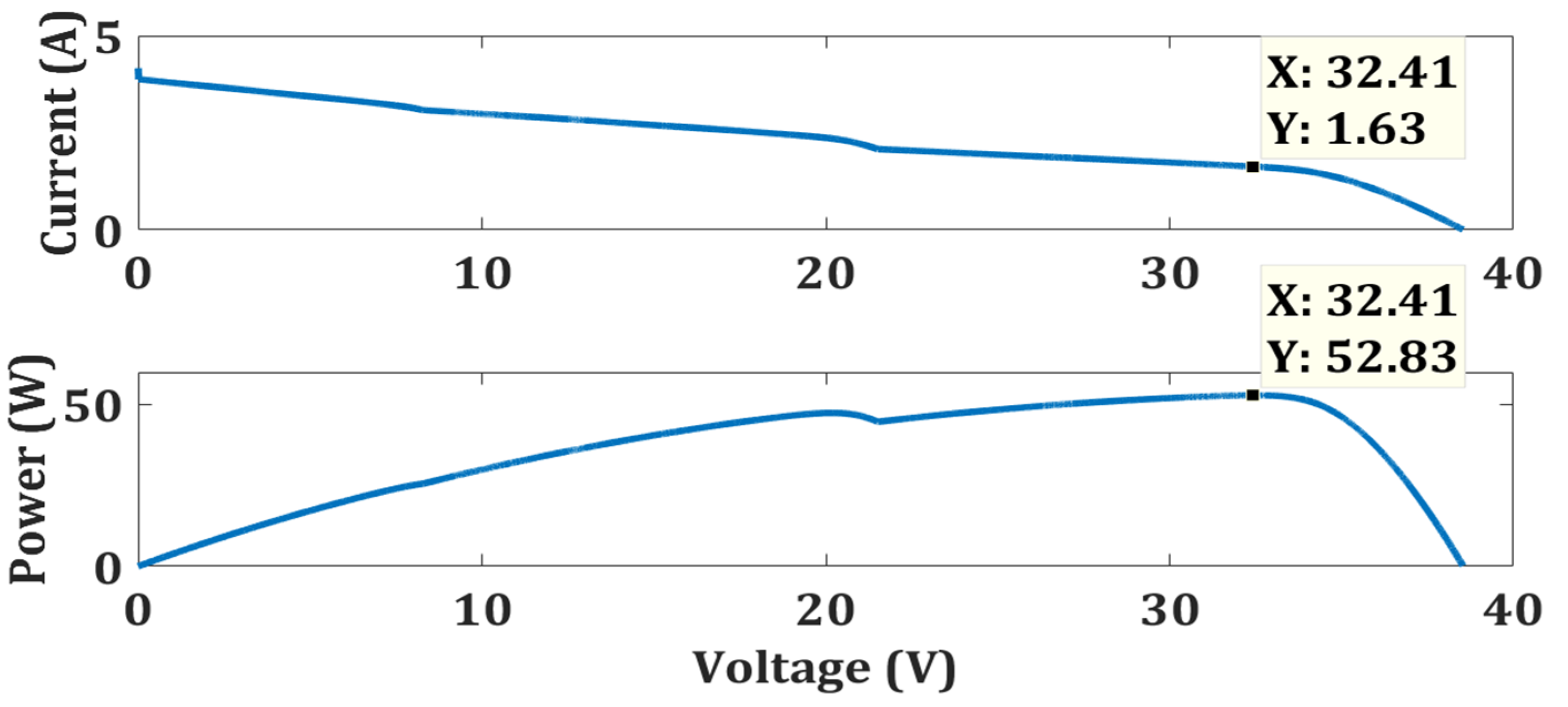
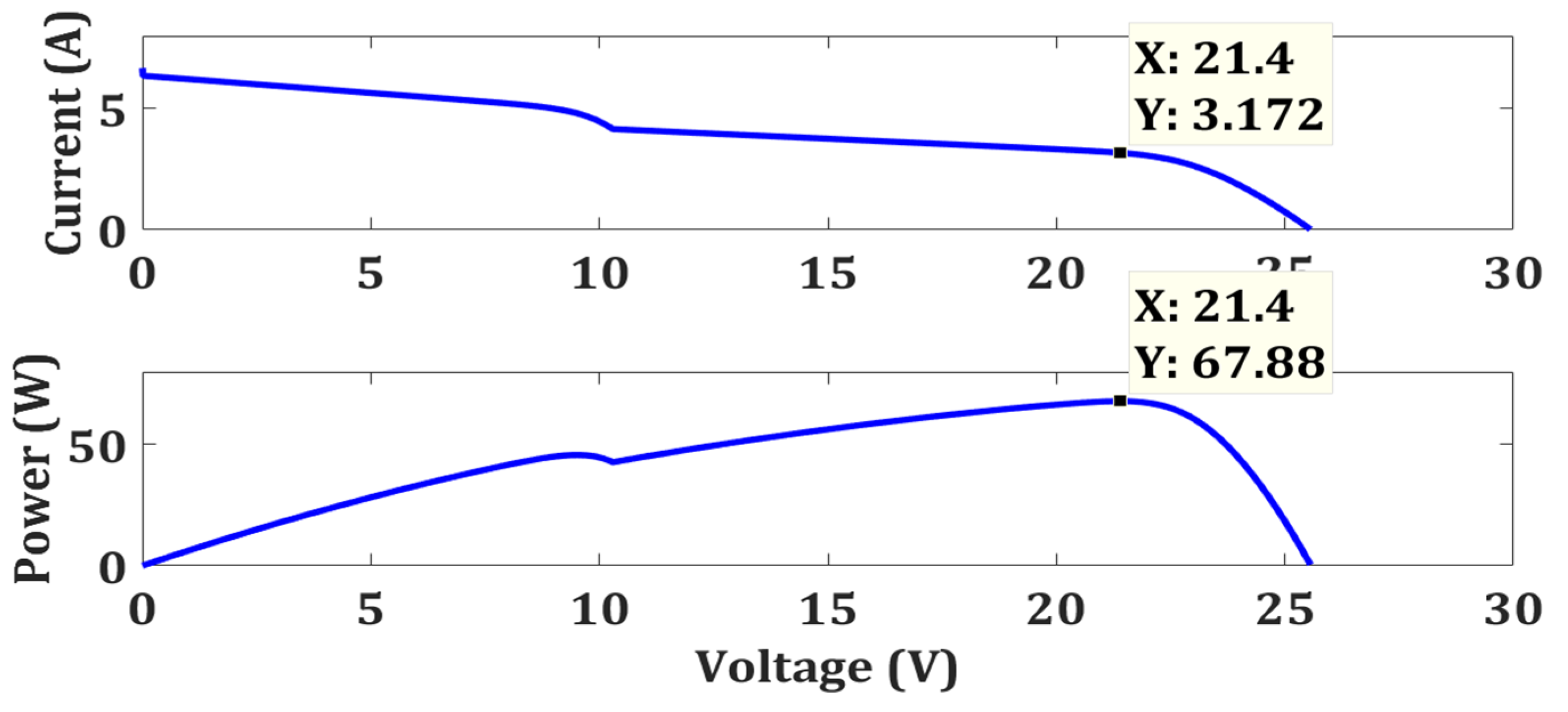
4.3. Strong Partial Shading
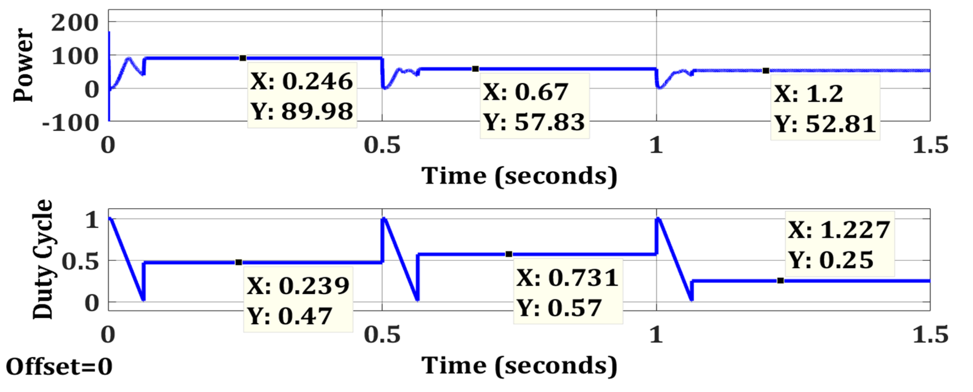
4.4. Changing Weather Condition
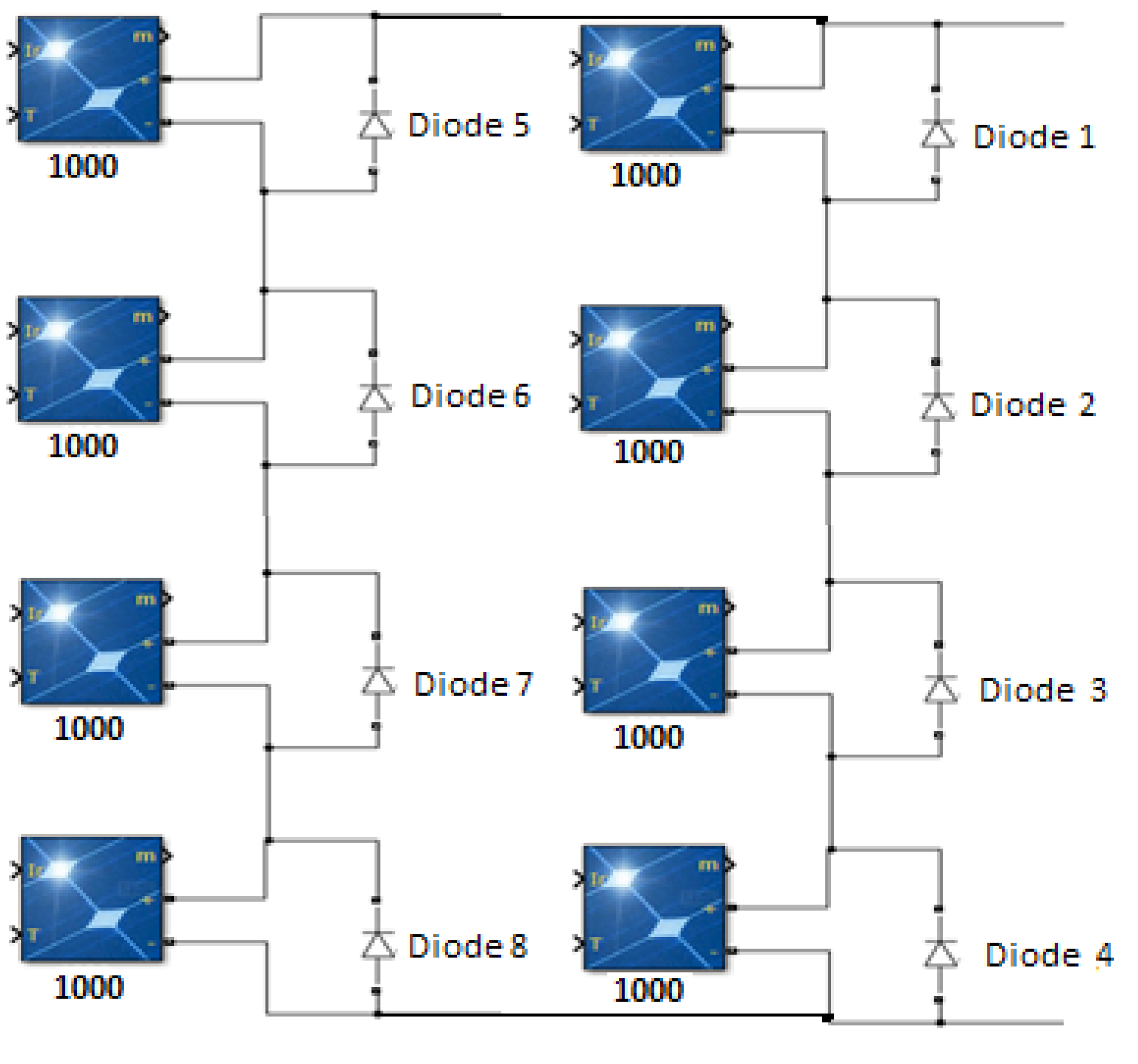
5. Two PV Strings Connected in Parallel (4S-2P)
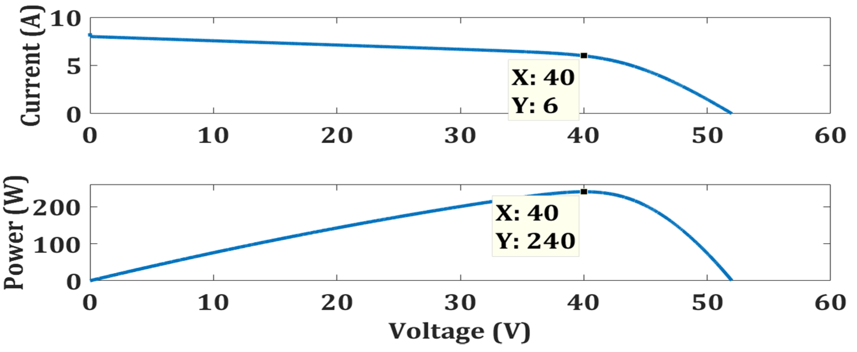
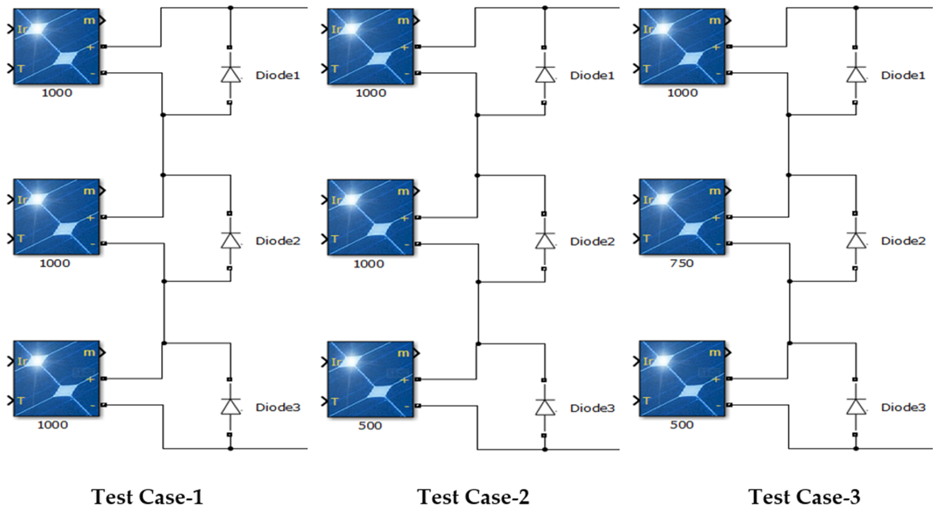
5.1. Zero Partial Shading at 4S2P PV System (Test Case 1)
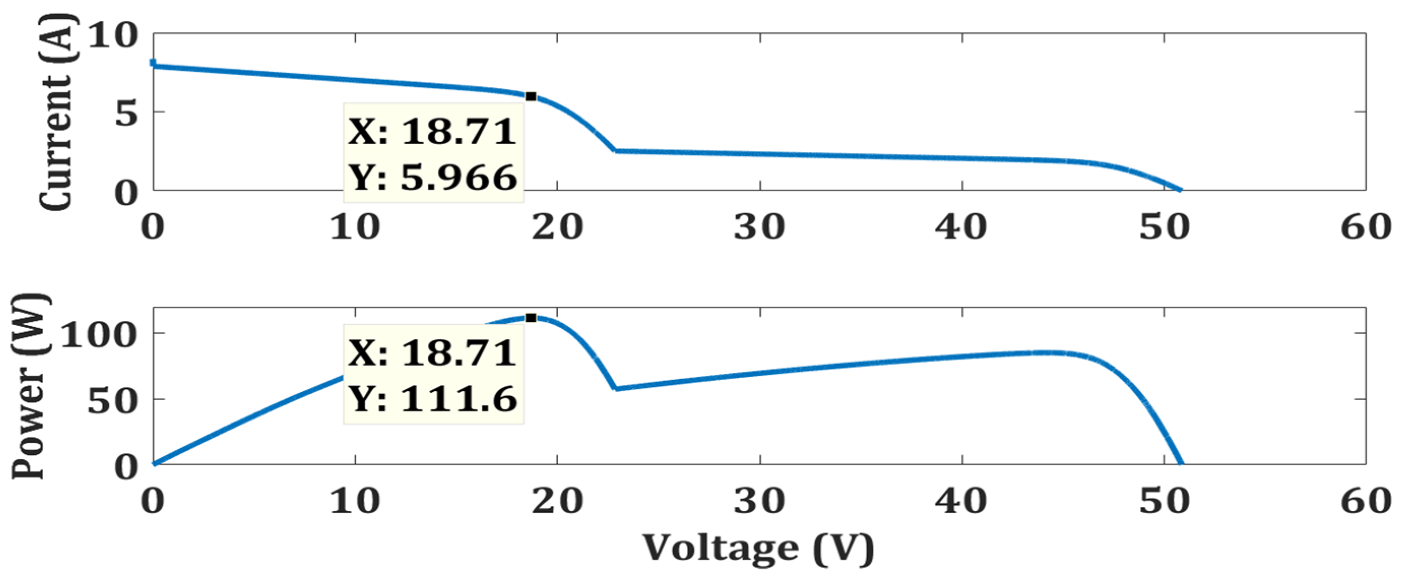
5.2. Weak Partial Shading at 4S2P PV System (Test Case 2)
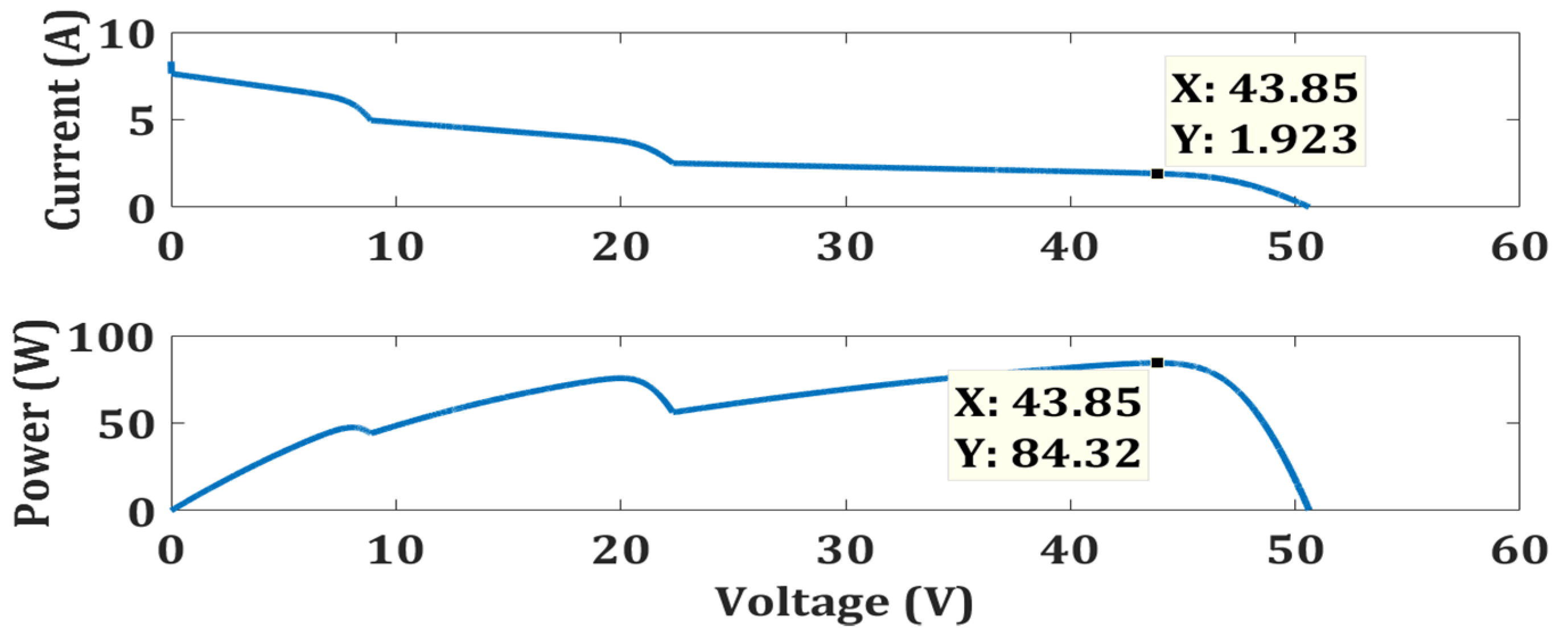
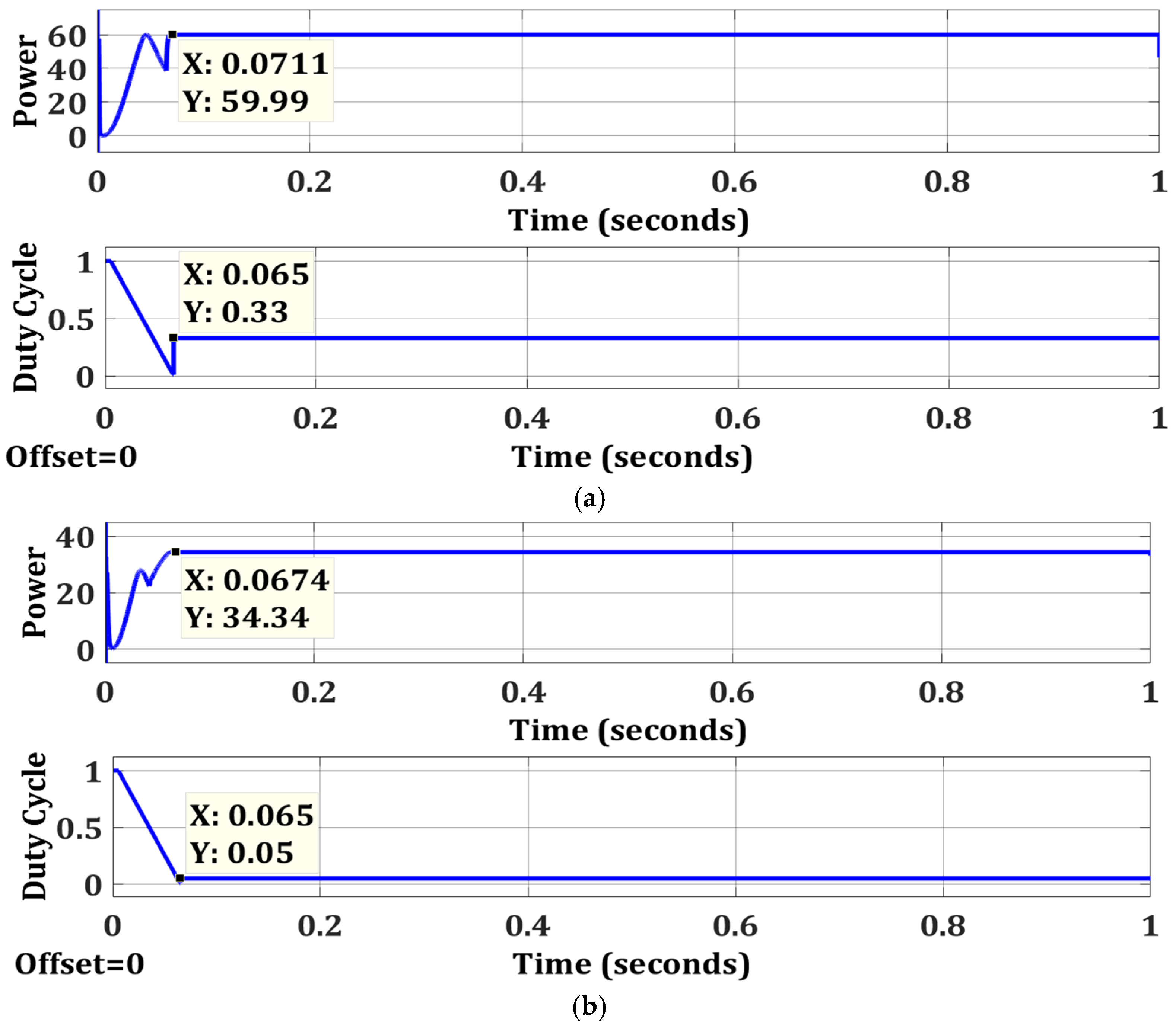
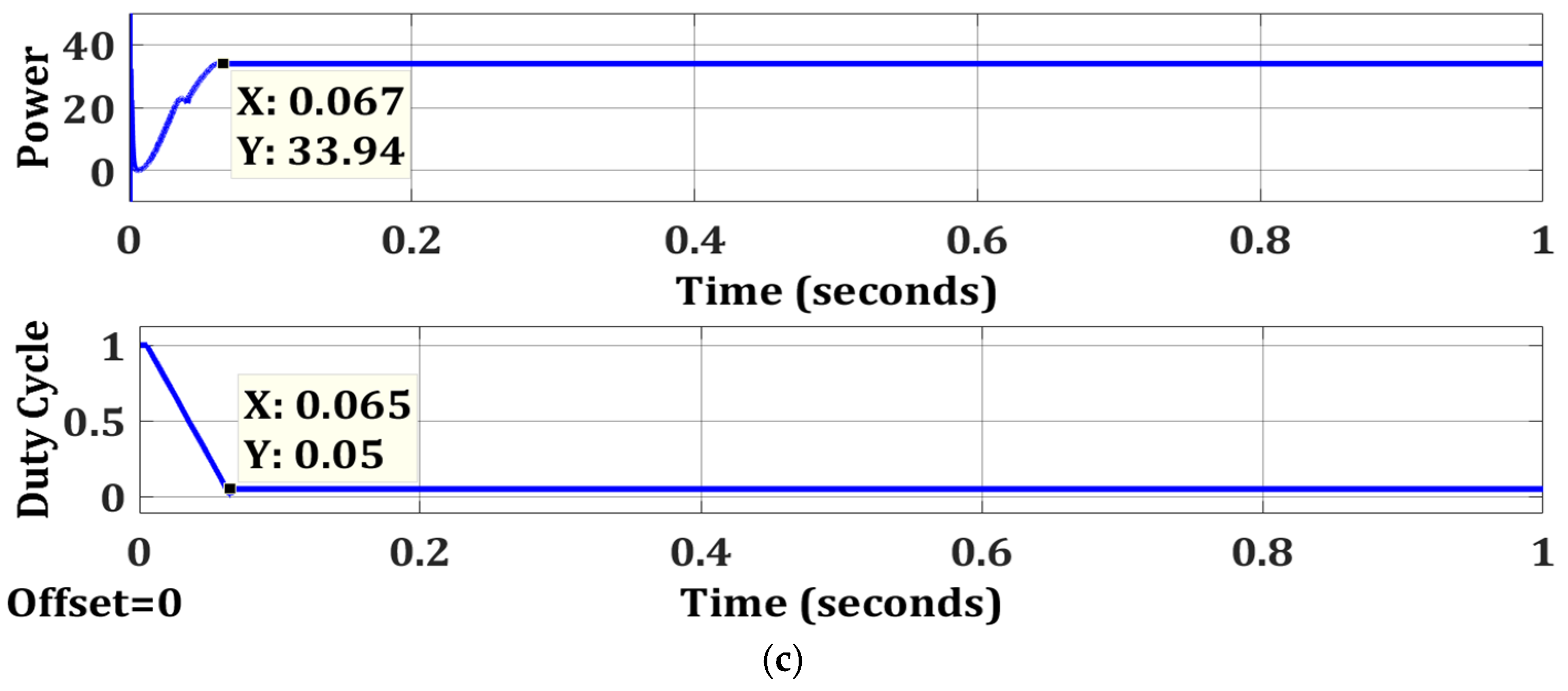
5.3. Strong Partial Shading Condition at 4S2P PV System
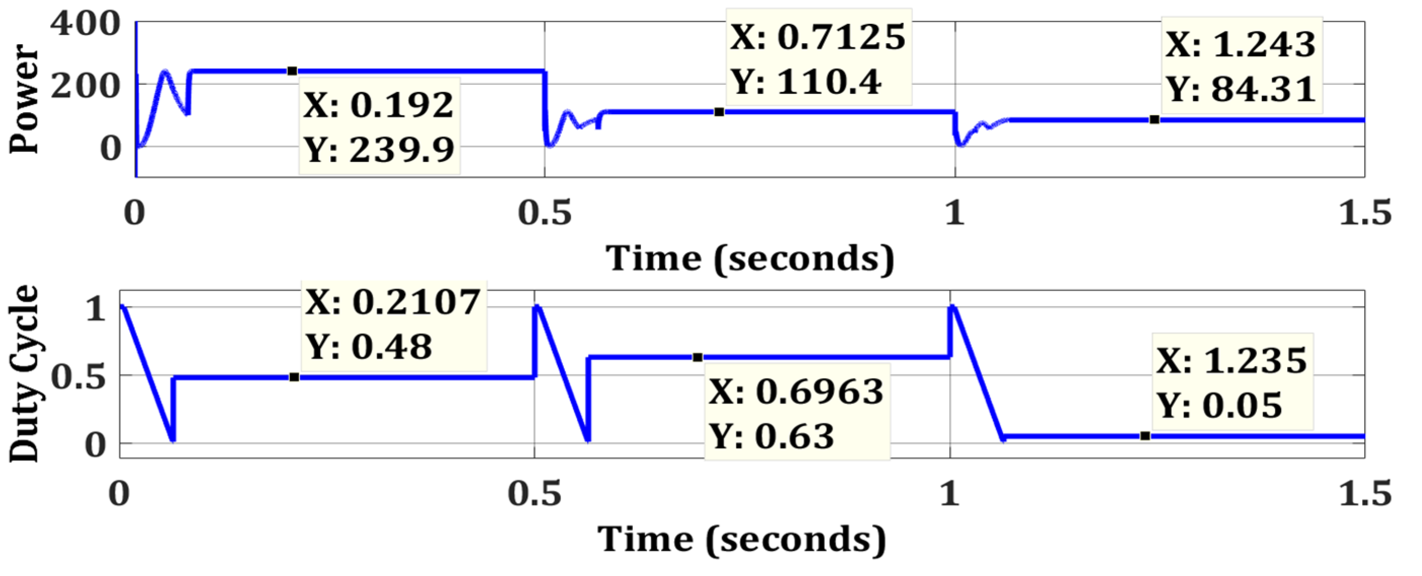
5.4. Changing Weather Conditions for 4S2P PV System
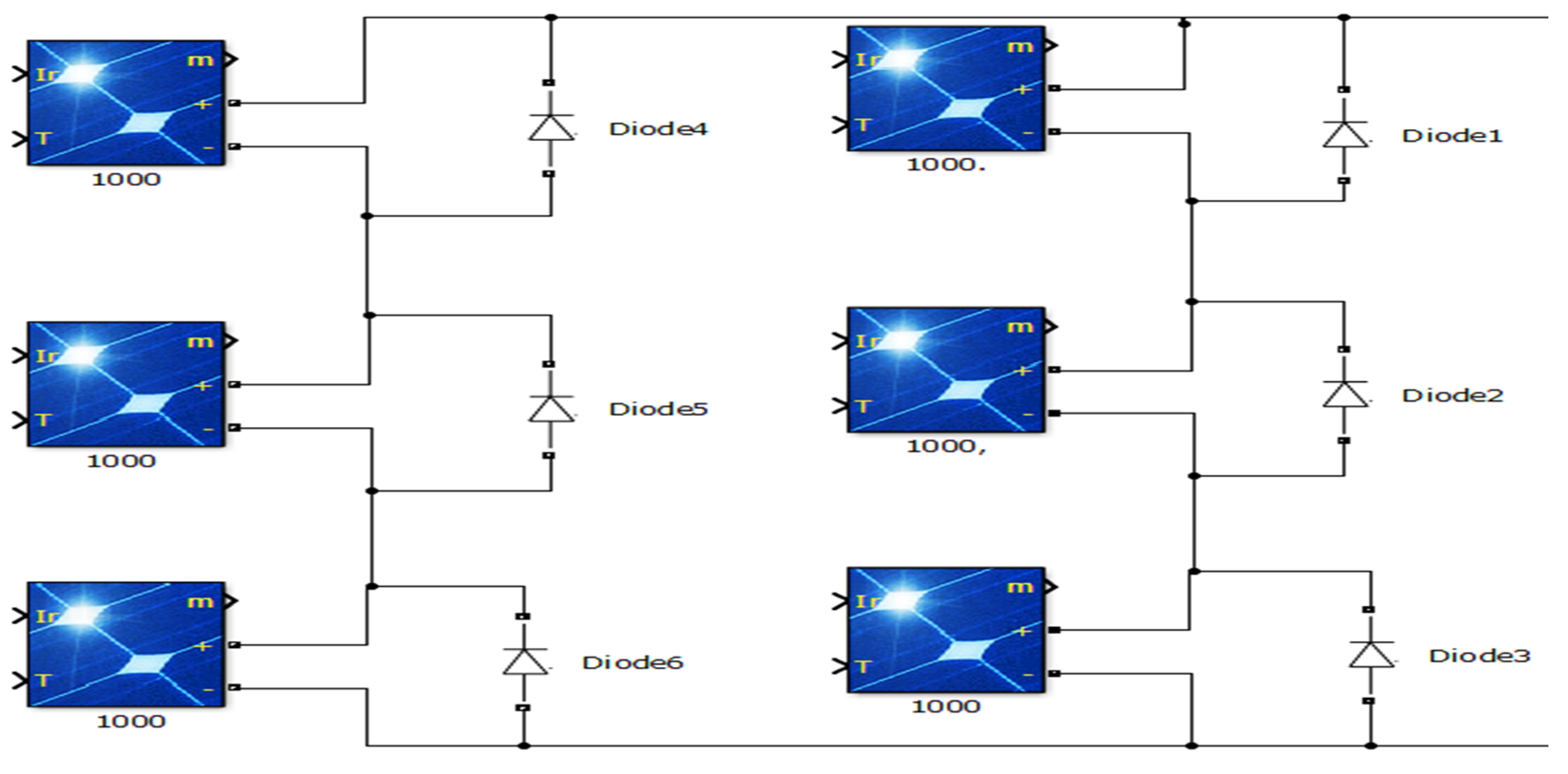
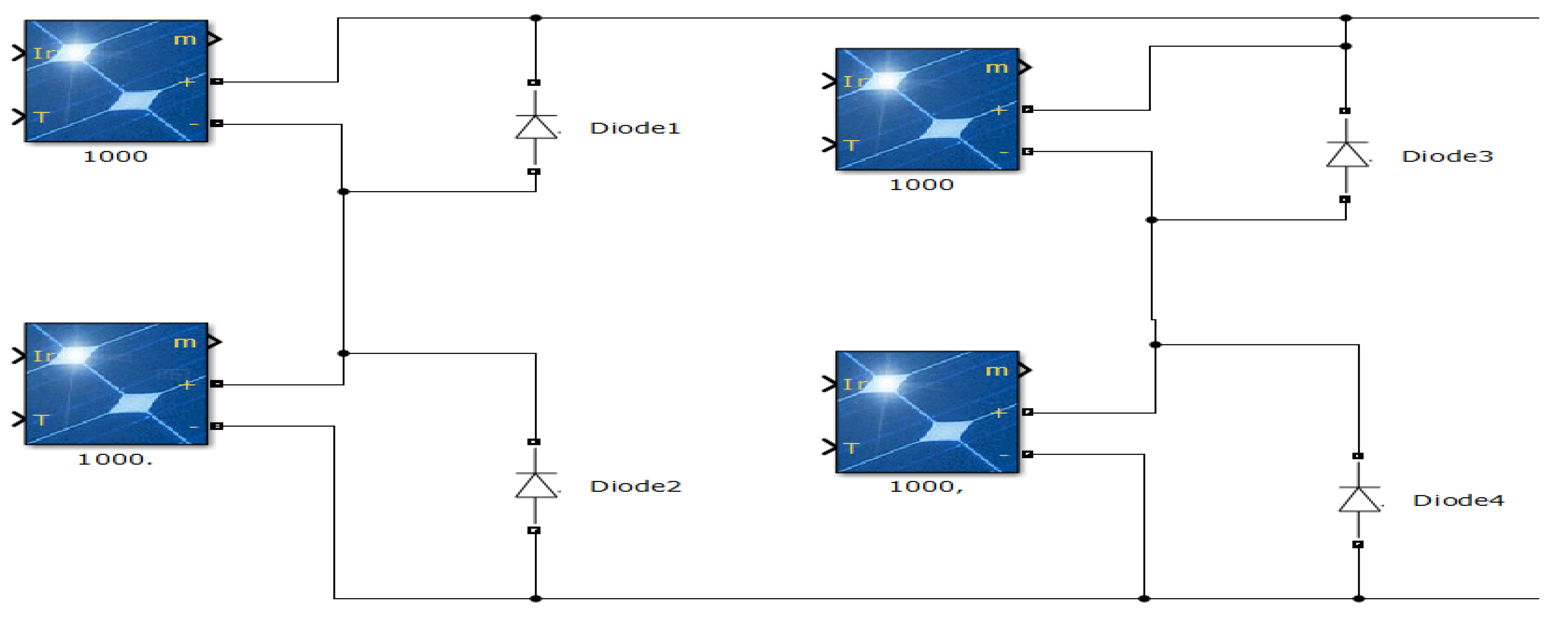
6. Three PV Modules Connected in Series (3S)
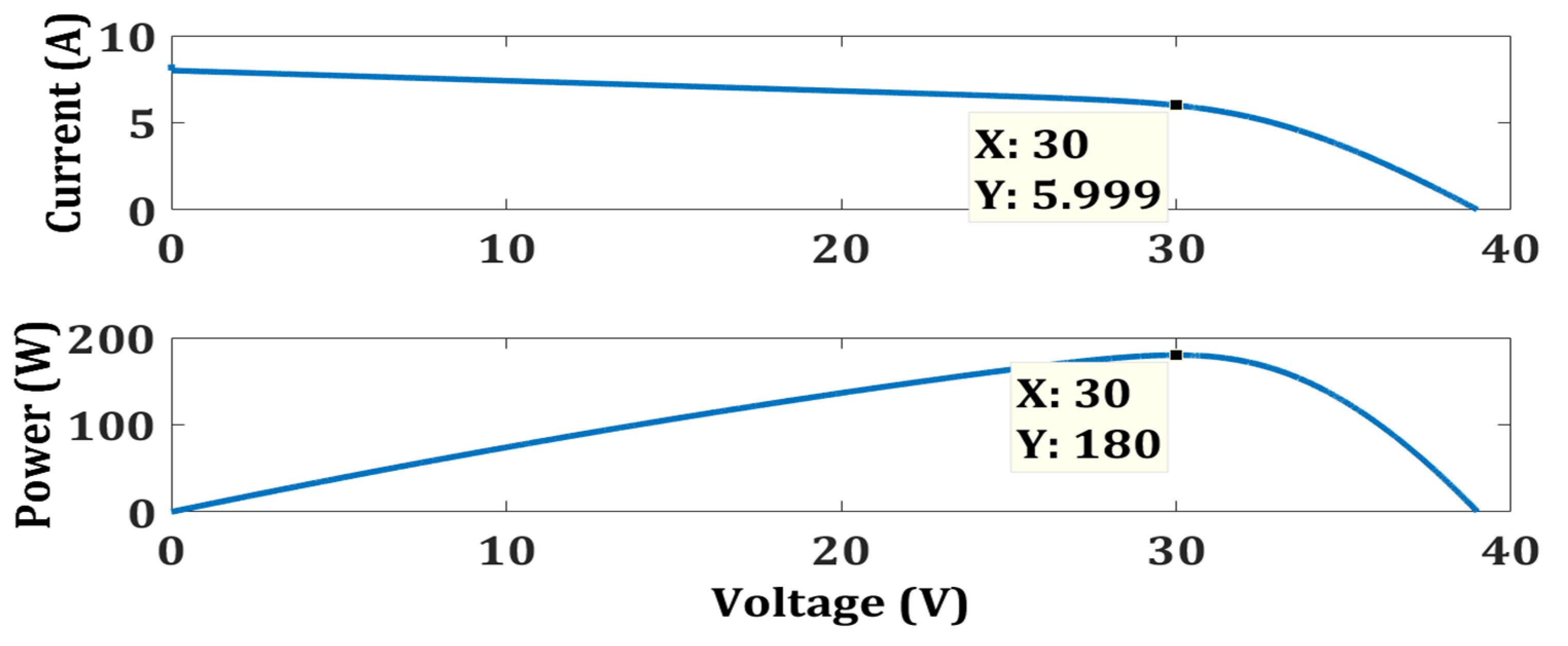
6.1. Zero Shading at 3S PV system (Test Case 1)
6.2. Weak Partial Shading at 3S PV System (Test Case 2)
6.3. Strong Partial Shading Condition at 3S PV System
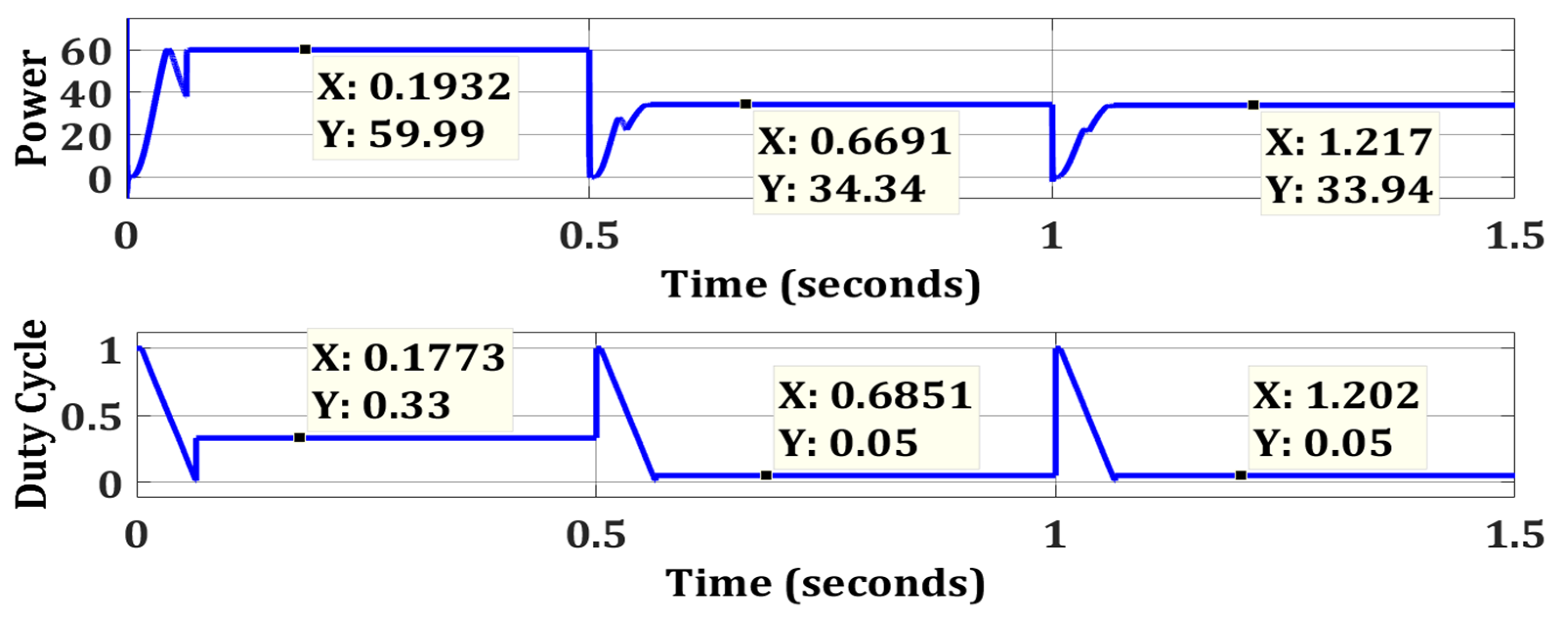
6.4. Changing Weather Conditions for 3S PV System
7. Two PV Strings Connected in Parallel (3S-2P)
7.1. No Shading at the PV System (Test Case 1)
7.2. Weak Partial Shading at 3S2P PV System (Test Case 2)
7.3. Strong Partial Shading Condition (Test Case 3)
7.4. Changing Weather Conditions for 3S2P PV System
8. Two PV Modules Connected in Series (2S)
8.1. Zero Shading at 2S PV System (Test Case 1)
8.2. Weak Partial Shading at 2S PV System (Test Case 2)
8.3. Strong Partial Shading Condition at 2S PV System
8.4. Changing Weather Conditions for 2S PV System
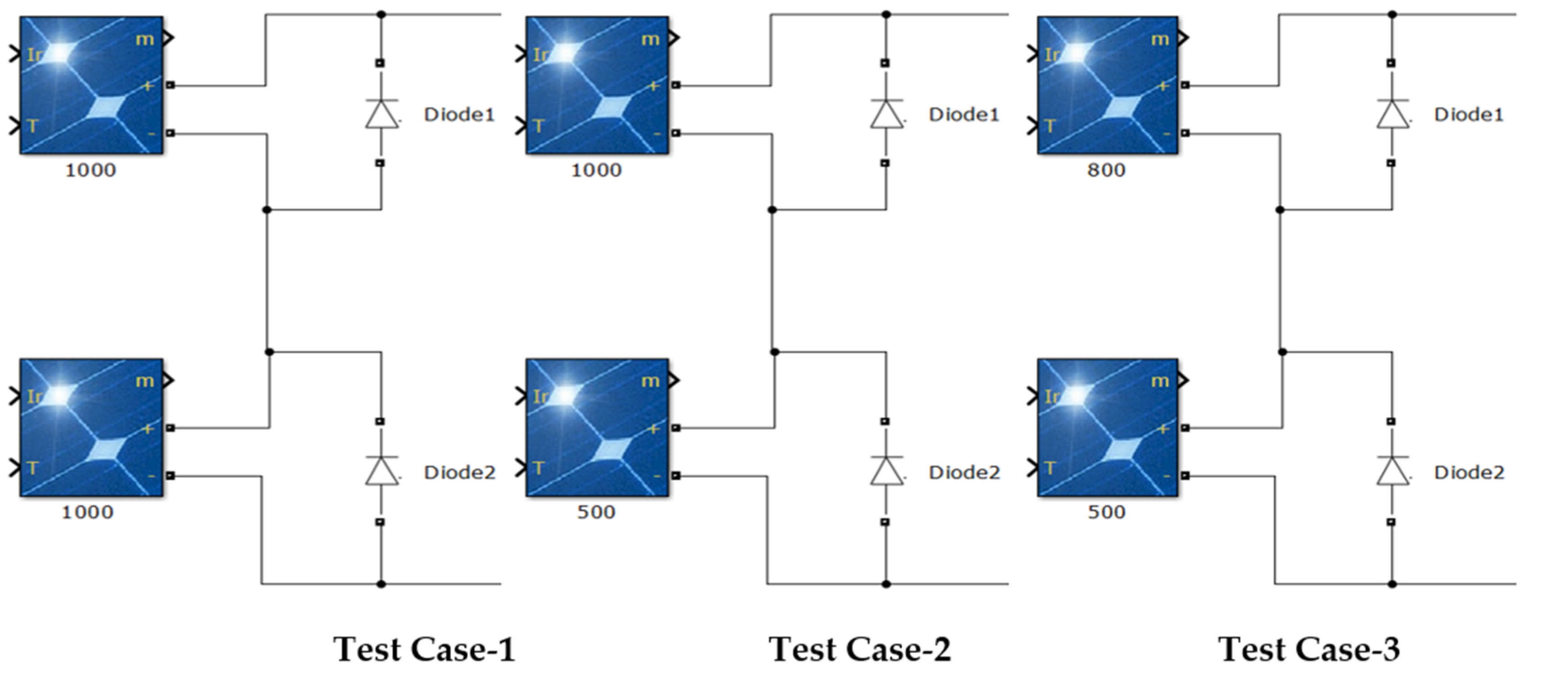
9. Two PV Strings Connected in Parallel (2S-2P)
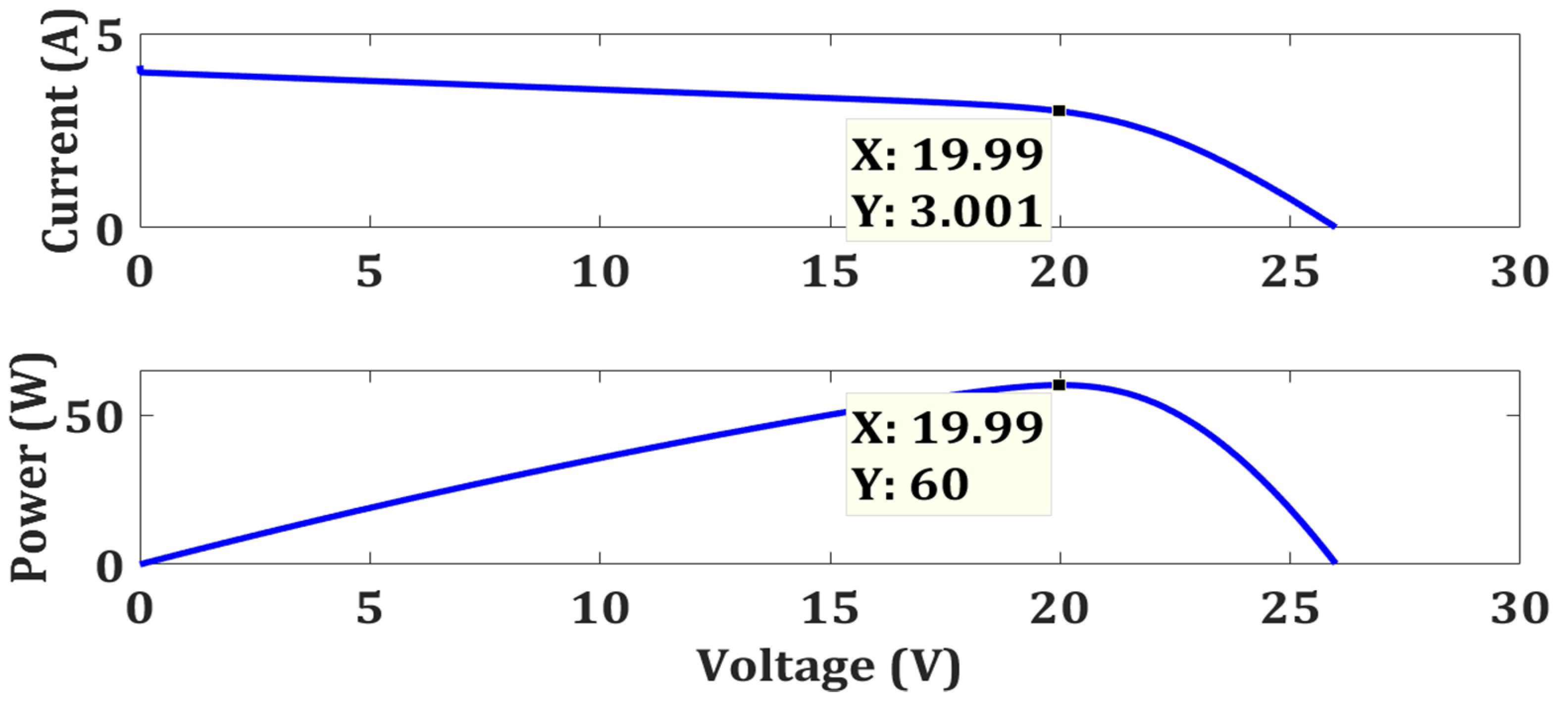
9.1. No Shading at the PV System (Test Case 1)
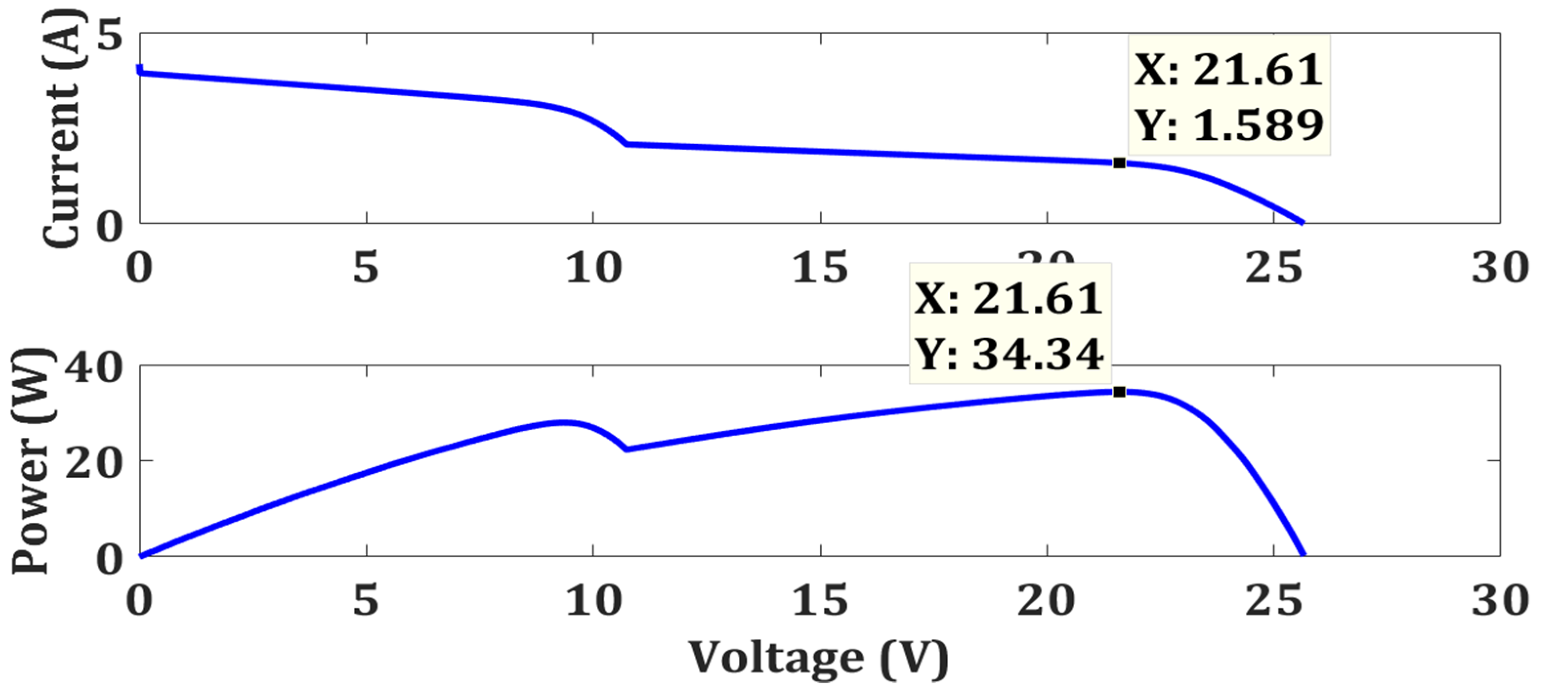
9.2. Weak Partial Shading at 2S2P PV System (Test Case 2)
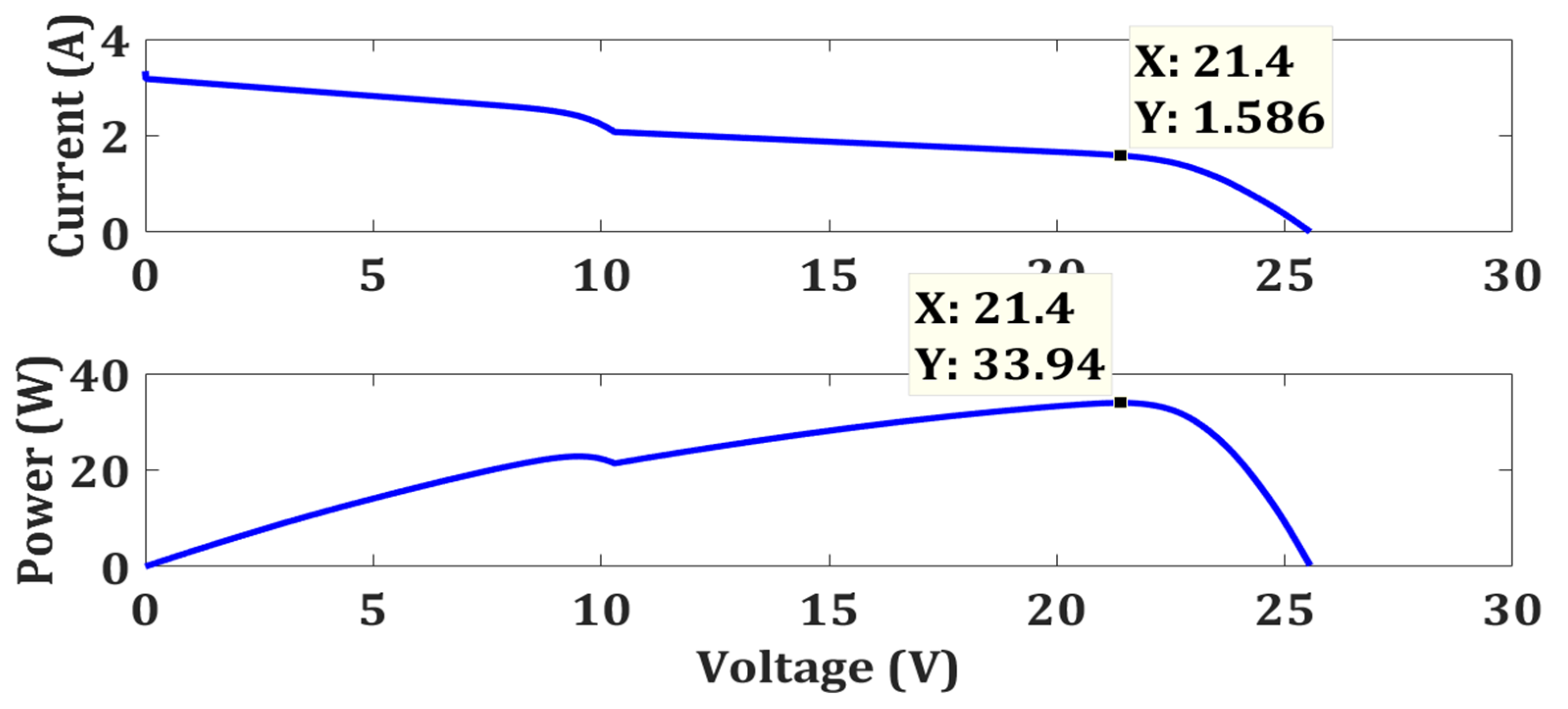
9.3. Strong Partial Shading Condition (Test Case 3)
9.4. Changing Weather Conditions for 2S2P PV System
10. Conclusions
Author Contributions
Funding
Institutional Review Board Statement
Informed Consent Statement
Data Availability Statement
Conflicts of Interest
References
- Ahmadi, M.H.; Ghazvini, M.; Sadeghzadeh, M.; Nazari, M.A.; Kumar, R.; Naeimi, A.; Ming, T. Solar power technology for electricity generation: A critical review. Energy Sci. Eng. 2018, 6, 340–361. [Google Scholar] [CrossRef] [Green Version]
- Rajput, P.; Malvoni, M.; Manoj Kumar, N.; Sastry, O.S.; Jayakumar, A. Operational performance and degradation influenced life cycle environmental–economic metrics of mc-Si, a-Si and HIT photovoltaic arrays in hot semi-arid climates. Sustainability 2020, 12, 1075. [Google Scholar] [CrossRef] [Green Version]
- Khatibi, A.; Astaraei, F.R.; Ahmadi, M.H. Generation and combination of the solar cells: A current model review. Energy Sci. Eng. 2019, 7, 305–322. [Google Scholar] [CrossRef] [Green Version]
- Awan, M.M.A.; Mahmood, T. Optimization of maximum power point tracking flower pollination algorithm for a standalone solar photovoltaic system. Mehran Univ. Res. J. Eng. Technol. 2020, 39, 267. [Google Scholar] [CrossRef]
- Başoğlu, M.E. A Fast GMPPT Algorithm Based on PV Characteristic for Partial Shading Conditions. Electronics 2019, 8, 1142. [Google Scholar] [CrossRef] [Green Version]
- Awan, M.M.A.; Awan, F.G. Improvement of maximum power point tracking perturb and observe algorithm for a standalone solar photovoltaic system. Mehran Univ. Res. J. Eng. Technol. 2017, 36, 501–510. [Google Scholar] [CrossRef] [Green Version]
- Feroz Mirza, A.; Mansoor, M.; Ling, Q.; Khan, M.I.; Aldossary, O.M. Advanced variable step size incremental conductance MPPT for a standalone PV system utilizing a GA-tuned PID controller. Energies 2020, 13, 4153. [Google Scholar] [CrossRef]
- Basha, C.H.; Rani, C. Different conventional and soft computing MPPT techniques for solar PV systems with high step-up boost converters: A comprehensive analysis. Energies 2020, 13, 371. [Google Scholar] [CrossRef] [Green Version]
- Debnath, A.; Olowu, T.O.; Parvez, I.; Dastgir, M.G.; Sarwat, A. A novel module independent straight line-based fast maximum power point tracking algorithm for photovoltaic systems. Energies 2020, 13, 3233. [Google Scholar] [CrossRef]
- Salam, Z.; Ahmed, J.; Merugu, B.S. The application of soft computing methods for MPPT of PV system: A technological and status review. Appl. Energy 2013, 107, 135–148. [Google Scholar] [CrossRef]
- Abdelsalam, A.K.; Massoud, A.M.; Ahmed, S.; Enjeti, P.N. High-Performance Adaptive Perturb and Observe MPPT Technique for Photovoltaic-Based Microgrids. IEEE Trans. Power Electron. 2011, 26, 1010–1021. [Google Scholar] [CrossRef]
- Ahmed, J.; Salam, Z. An improved perturb and observe (P&O) maximum power point tracking (MPPT) algorithm for higher efficiency. Appl. Energy 2015, 150, 97–108. [Google Scholar]
- Ishaque, K.; Salam, Z. A review of maximum power point tracking techniques of PV system for uniform insolation and partial shading condition. Renew. Sustain. Energy Rev. 2013, 19, 475–488. [Google Scholar] [CrossRef]
- Bastidas-Rodriguez, J.D.; Spagnuolo, G.; Franco, E.; Ramos-Paja, C.A.; Petrone, G. Maximum power point tracking architectures for photovoltaic systems in mismatching conditions: A review. IET Power Electron. 2014, 7, 1396–1413. [Google Scholar] [CrossRef]
- Xiao, W.; Dunford, W.G. A modified adaptive hill climbing MPPT method for photovoltaic power systems. In Proceedings of the 2004 IEEE 35th Annual Power Electronics Specialists Conference (IEEE Cat. No.04CH37551), Aachen, Germany, 20–25 June 2004; Volume 3, pp. 1957–1963. [Google Scholar]
- Zhou, Y.; Liu, F.; Yin, J.; Duan, S. Study on realizing MPPT by improved incremental conductance method with variable step-size. In Proceedings of the 2008 3rd IEEE Conference on Industrial Electronics and Applications, Singapore, 3–5 June 2008; pp. 547–550. [Google Scholar]
- Necaibia, S.; Kelaiaia, M.S.; Labar, H.; Necaibia, A. Implementation of an improved incremental conductance MPPT control based boost converter in photovoltaic applications. Int. J. Emerg. Electr. Power Syst. 2017, 18. [Google Scholar] [CrossRef]
- Sher, H.A.; Murtaza, A.F.; Noman, A.; Addoweesh, K.E.; Al-Haddad, K.; Chiaberge, M. A new sensorless hybrid MPPT algorithm based on fractional short-circuit current measurement and P&O MPPT. IEEE Trans. Sustain. Energy 2015, 6, 1426–1434. [Google Scholar]
- Baimel, D.; Tapuchi, S.; Levron, Y.; Belikov, J. Improved Fractional Open Circuit Voltage MPPT Methods for PV Systems. Electronics 2019, 8, 321. [Google Scholar] [CrossRef] [Green Version]
- Wang, Y.; Yang, Y.; Fang, G.; Zhang, B.; Wen, H.; Tang, H.; Fu, L.; Chen, X. An Advanced Maximum Power Point Tracking Method for Photovoltaic Systems by Using Variable Universe Fuzzy Logic Control Considering Temperature Variability. Electronics 2018, 7, 355. [Google Scholar] [CrossRef] [Green Version]
- Ilyas, A.; Ayyub, M.; Khan, M.R. Modelling and simulation of MPPT techniques for solar photovoltaic system using genetic algorithm optimised fuzzy logic controller. Int. J. Energy Technol. Policy 2020, 16, 174–195. [Google Scholar] [CrossRef]
- Basha, C.H.; Bansal, V.; Rani, C.; Brisilla, R.; Odofin, S. Development of Cuckoo Search MPPT Algorithm for Partially Shaded Solar PV SEPIC Converter. In Soft Computing for Problem Solving; Springer: Berlin/Heidelberg, Germany, 2020; pp. 727–736. [Google Scholar]
- Kinattingal, S.; Simon, S.P.; Nayak, P.S.R. MPPT in PV systems using ant colony optimisation with dwindling population. IET Renew. Power Gener. 2020, 14, 1105–1112. [Google Scholar]
- Tiwari, R.; Krishnamurthy, K.; Neelakandan, R.B.; Padmanaban, S.; Wheeler, P.W. Neural Network Based Maximum Power Point Tracking Control with Quadratic Boost Converter for PMSG—Wind Energy Conversion System. Electronics 2018, 7, 20. [Google Scholar] [CrossRef] [Green Version]
- Algarín, C.R.; Hernández, D.S.; Leal, D.R. A Low-Cost Maximum Power Point Tracking System Based on Neural Network Inverse Model Controller. Electronics 2018, 7, 4. [Google Scholar] [CrossRef] [Green Version]
- Zhang, P.; Sui, H. Maximum Power Point Tracking Technology of Photovoltaic Array under Partial Shading Based On Adaptive Improved Differential Evolution Algorithm. Energies 2020, 13, 1254. [Google Scholar] [CrossRef] [Green Version]
- da Luz, C.M.A.; Vicente, E.M.; Tofoli, F.L. Experimental evaluation of global maximum power point techniques under partial shading conditions. Sol. Energy 2020, 196, 49–73. [Google Scholar] [CrossRef]
- Wan, Y.; Mao, M.; Zhou, L.; Zhang, Q.; Xi, X.; Zheng, C. A Novel Nature-Inspired Maximum Power Point Tracking (MPPT) Controller Based on SSA-GWO Algorithm for Partially Shaded Photovoltaic Systems. Electronics 2019, 8, 680. [Google Scholar] [CrossRef] [Green Version]
- Pilakkat, D.; Kanthalakshmi, S. Single phase PV system operating under Partially Shaded Conditions with ABC-PO as MPPT algorithm for grid connected applications. Energy Rep. 2020, 6, 1910–1921. [Google Scholar] [CrossRef]
- Rajesh, R.; Mabel, M.C. Design and real time implementation of a novel rule compressed fuzzy logic method for the determination operating point in a photo voltaic system. Energy 2016, 116, 140–153. [Google Scholar] [CrossRef]
- Khanaki, R.; Radzi, M.A.M.; Marhaban, M.H. Comparison of ANN and P&O MPPT methods for PV applications under changing solar irradiation. In Proceedings of the 2013 IEEE Conference on Clean Energy and Technology (CEAT), Langkawi, Malaysia, 18–20 November 2013; pp. 287–292. [Google Scholar]
- Paul, S.; Thomas, J. Comparison of MPPT using GA optimized ANN employing PI controller for solar PV system with MPPT using incremental conductance. In Proceedings of the 2014 International Conference on Power Signals Control and Computations (EPSCICON), Thrissur, India, 6–11 January 2014; pp. 1–5. [Google Scholar]
- Chen, X.; Li, Y. A modified PSO structure resulting in high exploration ability with convergence guaranteed. IEEE Trans. Syst. Man Cybern. Part B (Cybern.) 2007, 37, 1271–1289. [Google Scholar] [CrossRef]
- Yousri, D.; Babu, T.S.; Allam, D.; Ramachandaramurthy, V.K.; Etiba, M.B. A Novel Chaotic Flower Pollination Algorithm for Global Maximum Power Point Tracking for Photovoltaic System under Partial Shading Conditions. IEEE Access 2019, 7, 121432–121445. [Google Scholar] [CrossRef]
- Javed, M.Y.; Mirza, A.F.; Hasan, A.; Rizvi, S.T.H.; Ling, Q.; Gulzar, M.M.; Safder, M.U.; Mansoor, M. A Comprehensive Review on a PV Based System to Harvest Maximum Power. Electronics 2019, 8, 1480. [Google Scholar] [CrossRef] [Green Version]
- Al-Majidi, S.D.; Abbod, M.F.; Al-Raweshidy, H.S. Design of an Efficient Maximum Power Point Tracker Based on ANFIS Using an Experimental Photovoltaic System Data. Electronics 2019, 8, 858. [Google Scholar] [CrossRef] [Green Version]
- Awan, M.M.A.; Mahmood, T. A Novel Ten Check Maximum Power Point Tracking Algorithm for a Standalone Solar Photovoltaic System. Electronics 2018, 7, 327. [Google Scholar] [CrossRef] [Green Version]
- Mousa, H.H.; Youssef, A.-R.; Mohamed, E.E. Variable step size P&O MPPT algorithm for optimal power extraction of multi-phase PMSG based wind generation system. Int. J. Electr. Power Energy Syst. 2019, 108, 218–231. [Google Scholar]
- Balaji, V.; Fathima, A.P. Enhancing the Maximum Power Extraction in Partially Shaded PV Arrays using Hybrid Salp Swarm Perturb and Observe Algorithm. Int. J. Renew. Energy Res. (IJRER) 2020, 10, 898–911. [Google Scholar]
- Zhang, S.; Wang, T.; Li, C.; Zhang, J.; Wang, Y. Maximum power point tracking control of solar power generation systems based on type-2 fuzzy logic. In Proceedings of the 2016 12th World Congress on Intelligent Control and Automation (WCICA), Guilin, China, 12–15 June 2016; pp. 770–774. [Google Scholar]
- Miyatake, M.; Veerachary, M.; Toriumi, F.; Fujii, N.; Ko, H. Maximum power point tracking of multiple photovoltaic arrays: A PSO approach. IEEE Trans. Aerosp. Electron. Syst. 2011, 47, 367–380. [Google Scholar] [CrossRef]

| Strengths | Weaknesses | Opportunities | Threats |
|---|---|---|---|
| Simple structure | Hard to implement. | Improvement in tracking speed | Nil |
| No huge computations | High settling time | Improvement in tracking accuracy | |
| Easy implementation | Minimize the settling time to reduce the tracking time | ||
| Fast tracking speed | |||
| No parameter to tune | |||
| Ability to differentiate MPP and GMPP | |||
| Efficient performance under all weather conditions | |||
| Independent of PV system | |||
| Zero steady-state oscillations |
| Optimized Ten Check Algorithm | Ten Check Algorithm |
|---|---|
| A | A |
| B | B |
| Shading Patterns | Algorithms | PMPP (W) | Rated Power (W) | Efficiency (%) | Tracking Time (s) | Increase in Tracking Speed (%) |
|---|---|---|---|---|---|---|
| Zero Shading | TCA | 119.7 | 120 | 99.75 | 0.4972 | 86.3 |
| FPA | 119.2 | 99.33 | 0.7516 | 90.93 | ||
| OTCA | 120 | 100 | 0.0682 |
| Shading Patterns | Algorithms | PMPP (W) | Rated Power (W) | Efficiency (%) | Tracking Time (s) | Increase in Tracking Speed (%) |
|---|---|---|---|---|---|---|
| Weak Partial Shading | TCA | 55.78 | 55.81 | 99.955 | 0.497 | 85.7 |
| FPA | 55.24 | 98.98 | 0.7565 | 90.61 | ||
| OTCA | 55.71 | 99.82 | 0.071 |
| Shading Patterns | Algorithms | PMPP (W) | Rated Power (W) | Efficiency (%) | Tracking Time (s) | Increase in Tracking Speed (%) |
|---|---|---|---|---|---|---|
| Strong Partial Shading | TCA | 42.16 | 42.16 | 100 | 0.4972 | 86.7 |
| FPA | 42.05 | 99.74 | 0.7527 | 91.23 | ||
| OTCA | 42.15 | 99.98 | 0.066 |
| Shading Patterns | Algorithms | PMPP (W) | Rated Power (W) | Efficiency (%) | Tracking Time (s) | Increase in Tracking Speed (%) |
|---|---|---|---|---|---|---|
| Zero Shading | TCA | 119.7 | 120 | 99.75 | 0.4972 | 86.3 |
| FPA | 119.2 | 99.33 | 0.7516 | 90.93 | ||
| OTCA | 120 | 100 | 0.0682 | |||
| Weak Partial Shading | TCA | 55.78 | 55.81 | 99.955 | 0.497 | 85.7 |
| FPA | 55.24 | 98.98 | 0.7565 | 90.61 | ||
| OTCA | 55.71 | 99.82 | 0.071 | |||
| Strong Partial Shading | TCA | 42.16 | 42.16 | 100 | 0.4972 | 86.7 |
| FPA | 42.05 | 99.74 | 0.7527 | 91.23 | ||
| OTCA | 42.15 | 99.98 | 0.066 |
| Partial Shading | Algorithms | Algorithms | Structural Complexity | Power (W) | Rated Power (W) | Efficiency (%) | Tracking Speed (s) |
|---|---|---|---|---|---|---|---|
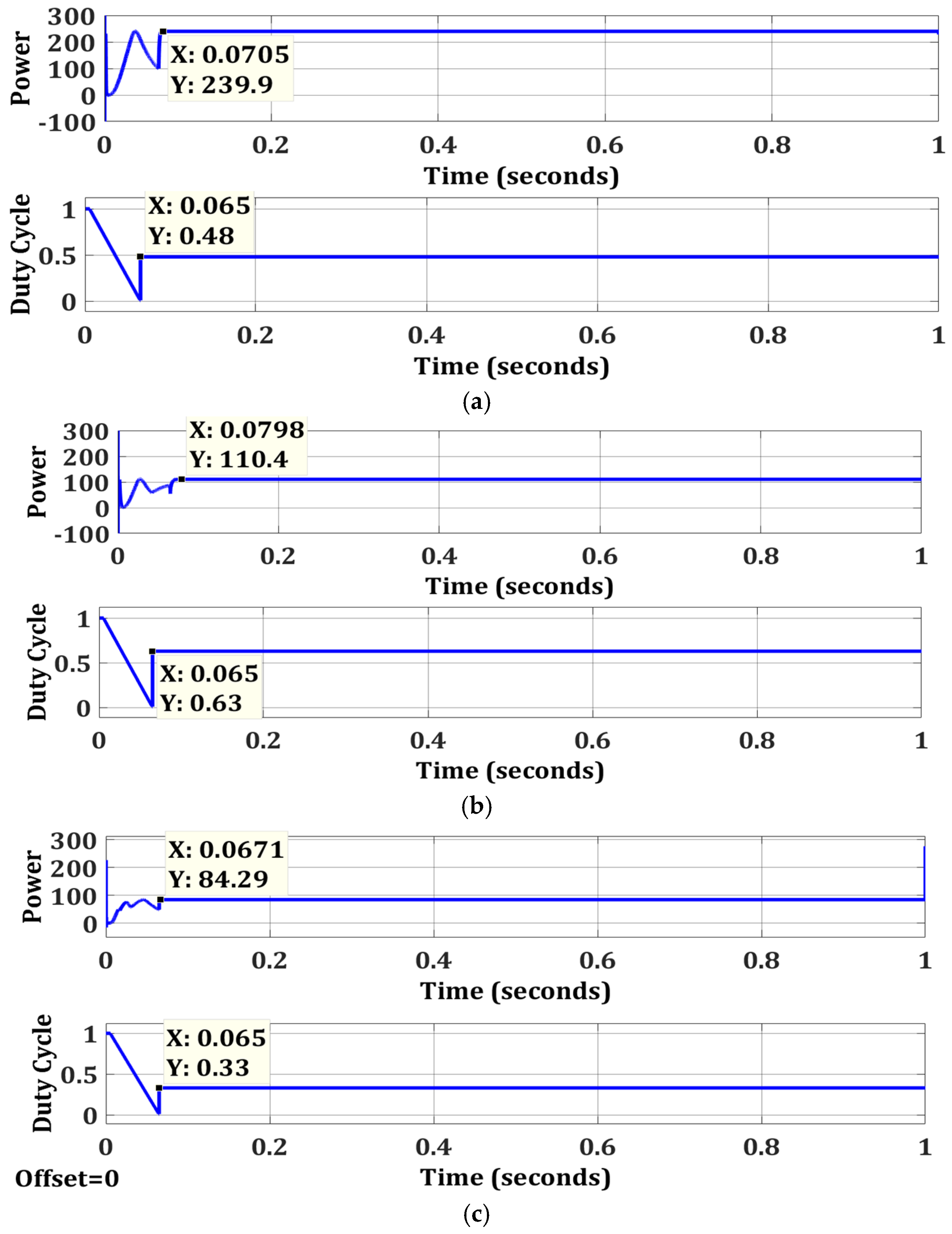
| Test Case 1 | OTCA | Ten Check | Simple | 239.9 | 240 | 99.96 | 0.0705 |
| Test Case 2 | OTCA | Ten Check | Simple | 110.4 | 111.6 | 98.92 | 0.0798 |
| Test Case 3 | OTCA | Ten Check | Simple | 84.29 | 84.32 | 99.96 | 0.0671 |
| Partial Shading | Algorithms | Structural Complexity | Oscillations | Power (W) | Rated Power (W) | Efficiency (%) | Tracking Speed (s) |
|---|---|---|---|---|---|---|---|
| Case 1 | OTCA | Simple | No | 89.98 | 90 | 99.98 | 0.069 |
| Case 2 | OTCA | Simple | No | 57.83 | 57.9 | 99.88 | 0.0732 |
| Case 3 | OTCA | Simple | No | 52.81 | 52.83 | 99.96 | 0.065 |
| Partial Shading | Algorithms | Structural Complexity | Oscillations | Power (W) | Rated Power (W) | Efficiency (%) | Tracking Speed (sec) |
|---|---|---|---|---|---|---|---|
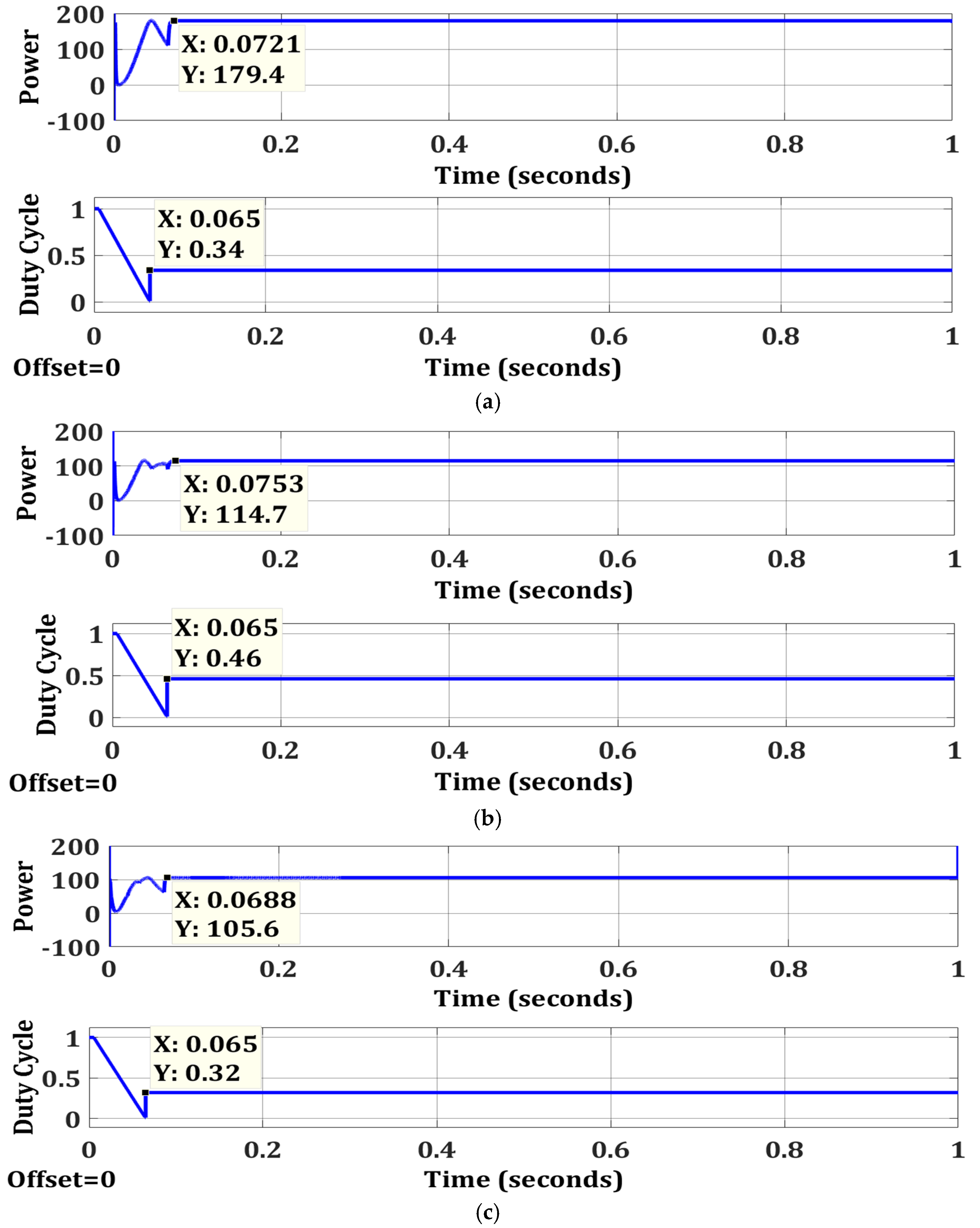
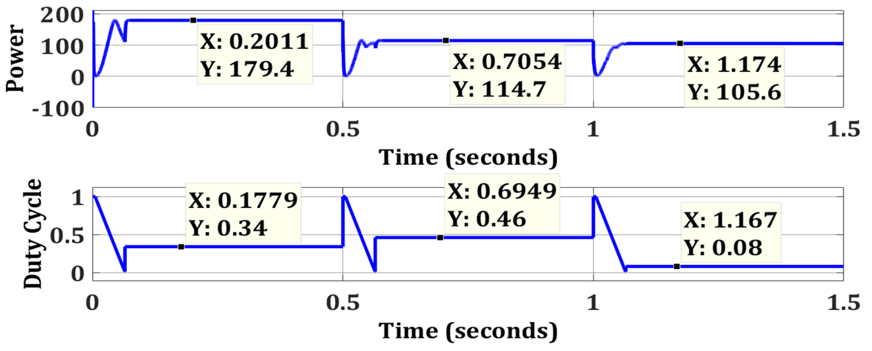
| Case 1 | OTCA | Simple | No | 179.4 | 180 | 99.67 | 0.0721 |
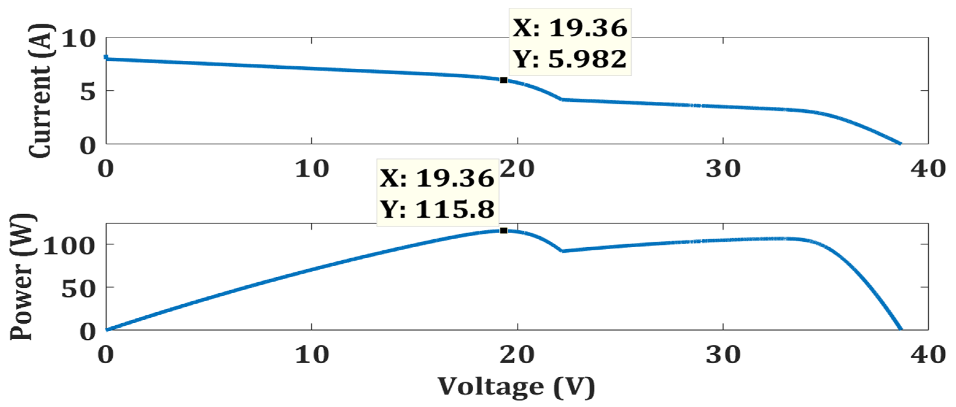
| Case 2 | OTCA | Simple | No | 114.7 | 115.8 | 99.05 | 0.0753 |
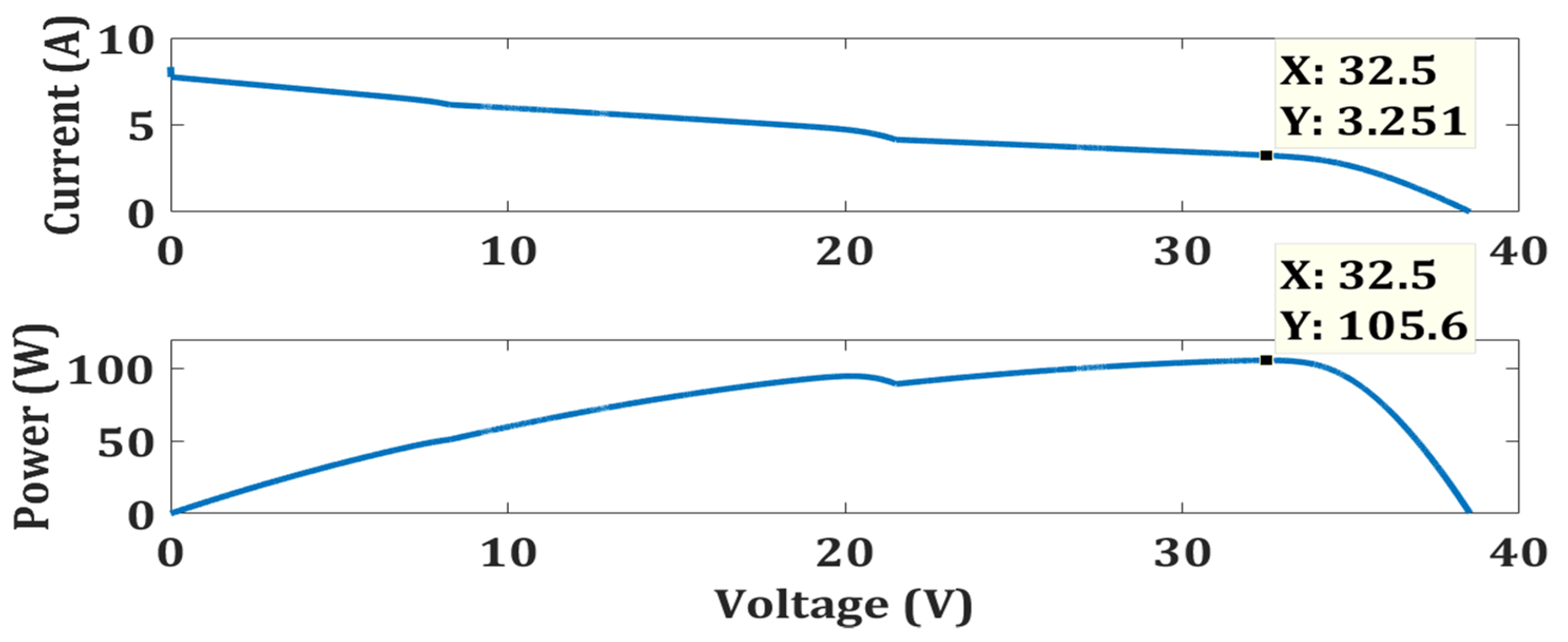
| Case 3 | OTCA | Simple | No | 105.6 | 105.6 | 100 | 0.0688 |
| Partial Shading | Algorithms | Structural Complexity | Oscillations | Power (W) | Rated Power (W) | Efficiency (%) | Tracking Speed (s) |
|---|---|---|---|---|---|---|---|
| Case 1 | OTCA | Simple | No | 59.99 | 60 | 99.98 | 0.0711 |
| Case 2 | OTCA | Simple | No | 34.34 | 34.34 | 100 | 0.0674 |
| Case 3 | OTCA | Simple | No | 33.94 | 33.94 | 100 | 0.067 |
| Partial Shading | Algorithms | Structural Complexity | Oscillations | Power (W) | Rated Power (W) | Efficiency (%) | Tracking Speed (sec) |
|---|---|---|---|---|---|---|---|
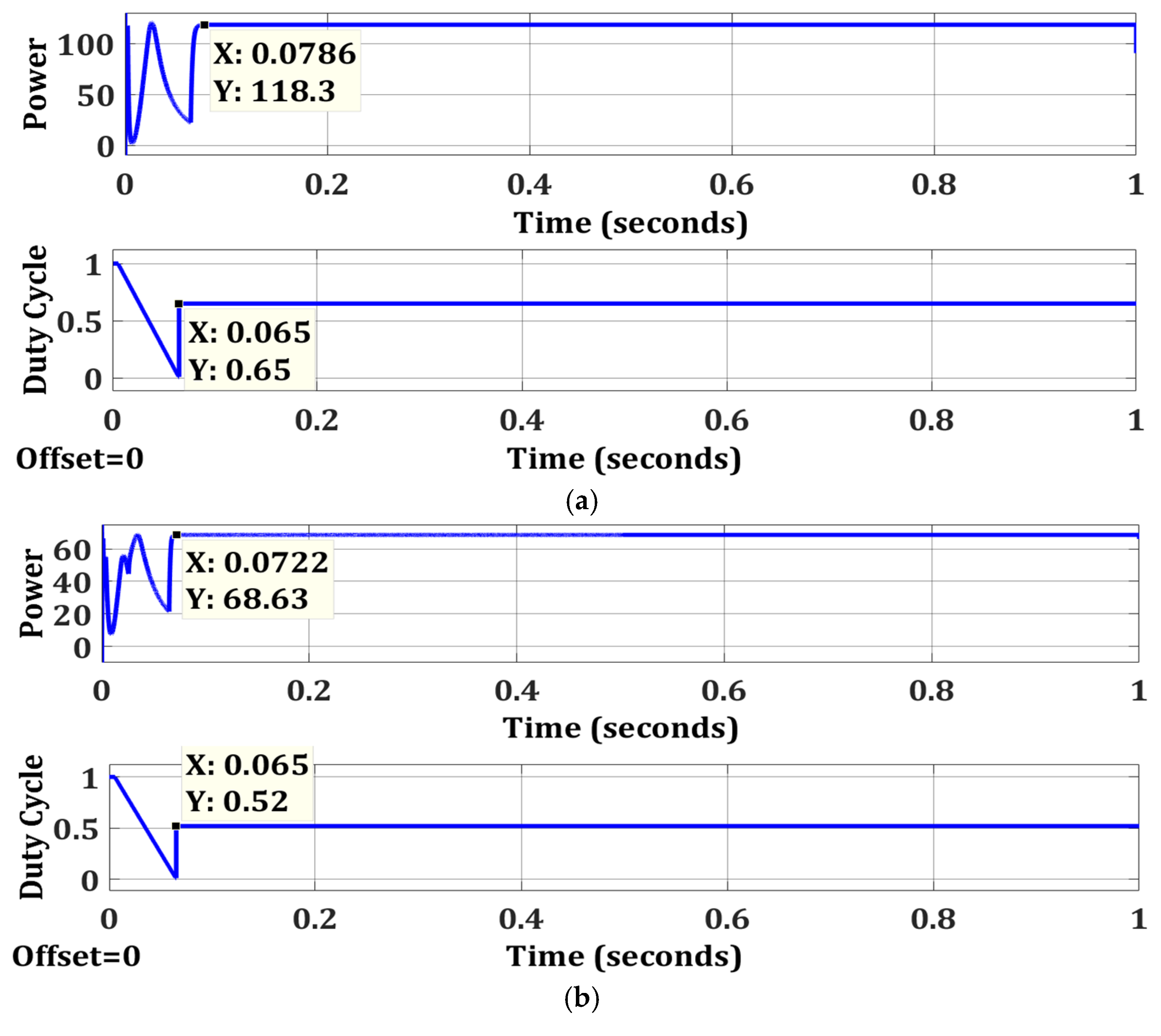
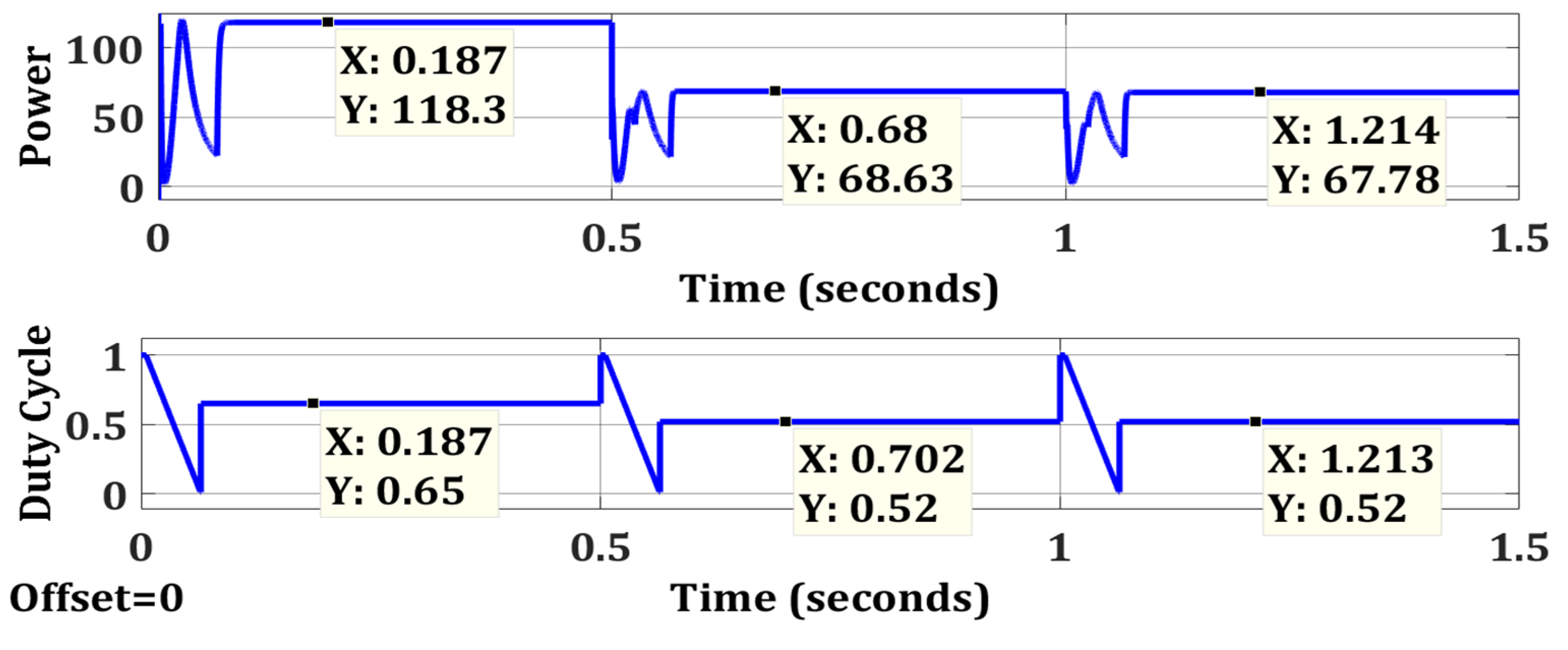
| Case 1 | OTCA | Simple | No | 118.3 | 120 | 98.58 | 0.0786 |
| Case 2 | OTCA | Simple | No | 68.63 | 68.67 | 99.94 | 0.0722 |
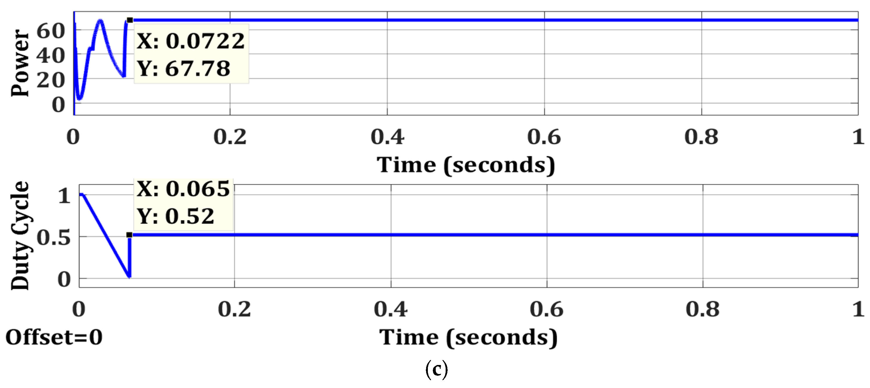
| Case 3 | OTCA | Simple | No | 67.78 | 67.88 | 99.85 | 0.0722 |
| Sr. N0. | Algorithms | FPA [4] | TCA [37] | P&O [38,39] | Fuzzy [40] | PSO [41] | OTCA |
|---|---|---|---|---|---|---|---|
| Parameters | |||||||
| 1 | Steady State Oscillations | Zero | Zero | High | Low | Zero | Zero |
| 2 | Tracking Speed | Fast | Faster | Low | Adequate | Adequate | FASTEST |
| 3 | Procedural Complications | Reasonable | Nil | Less | High | Reasonable | Nil |
| 4 | Memorizing Necessity | Few | Few | Few | Large | Few | FEW |
| 5 | Computational Complications | Average | No | Zero | High | Average | No |
| 6 | Implementation | Hard | Moderate | Easy | Hard | Hard | Easy |
| 7 | Performance in PSC | Good | Very Good | N/A | Good | Good | EXCELLENT |
| 8 | Module Dependent | No | No | Yes | Yes | No | No |
| 9 | Efficiency | Effective | High | Fail | Low under PSC | Effective | Exciting |
| 10 | Structure | Complex | Simple | Simple | Complex | Complex | Simple |
Publisher’s Note: MDPI stays neutral with regard to jurisdictional claims in published maps and institutional affiliations. |
© 2022 by the authors. Licensee MDPI, Basel, Switzerland. This article is an open access article distributed under the terms and conditions of the Creative Commons Attribution (CC BY) license (https://creativecommons.org/licenses/by/4.0/).
Share and Cite
Awan, M.M.A.; Javed, M.Y.; Asghar, A.B.; Ejsmont, K. Performance Optimization of a Ten Check MPPT Algorithm for an Off-Grid Solar Photovoltaic System. Energies 2022, 15, 2104. https://doi.org/10.3390/en15062104
Awan MMA, Javed MY, Asghar AB, Ejsmont K. Performance Optimization of a Ten Check MPPT Algorithm for an Off-Grid Solar Photovoltaic System. Energies. 2022; 15(6):2104. https://doi.org/10.3390/en15062104
Chicago/Turabian StyleAwan, Muhammad Mateen Afzal, Muhammad Yaqoob Javed, Aamer Bilal Asghar, and Krzysztof Ejsmont. 2022. "Performance Optimization of a Ten Check MPPT Algorithm for an Off-Grid Solar Photovoltaic System" Energies 15, no. 6: 2104. https://doi.org/10.3390/en15062104
APA StyleAwan, M. M. A., Javed, M. Y., Asghar, A. B., & Ejsmont, K. (2022). Performance Optimization of a Ten Check MPPT Algorithm for an Off-Grid Solar Photovoltaic System. Energies, 15(6), 2104. https://doi.org/10.3390/en15062104