
Vibration Reduction System with a Linear Motor: Operation Modes, Dynamic Performance, Energy Consumption


Abstract
:1. Introduction
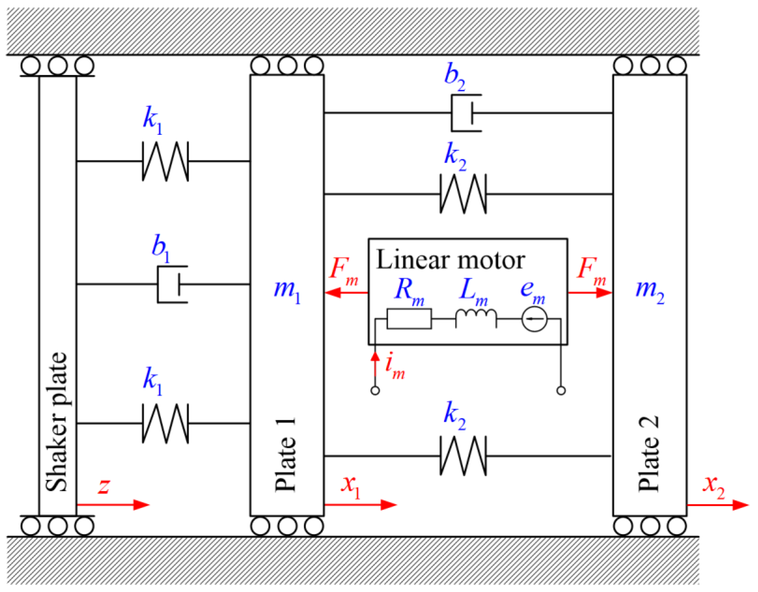
2. Vibration Reduction System
3. Modelling
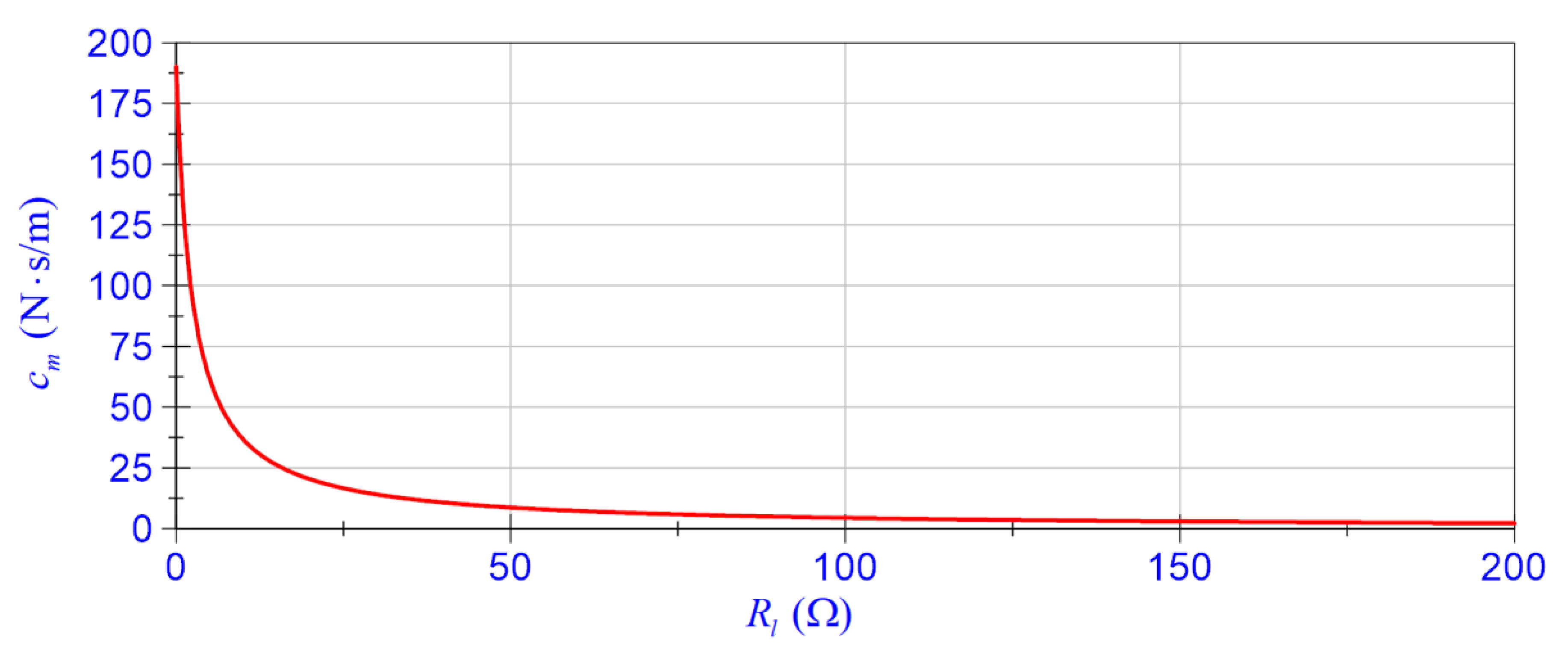
3.1. Passive and Semi-Active Mode
3.2. Active Mode
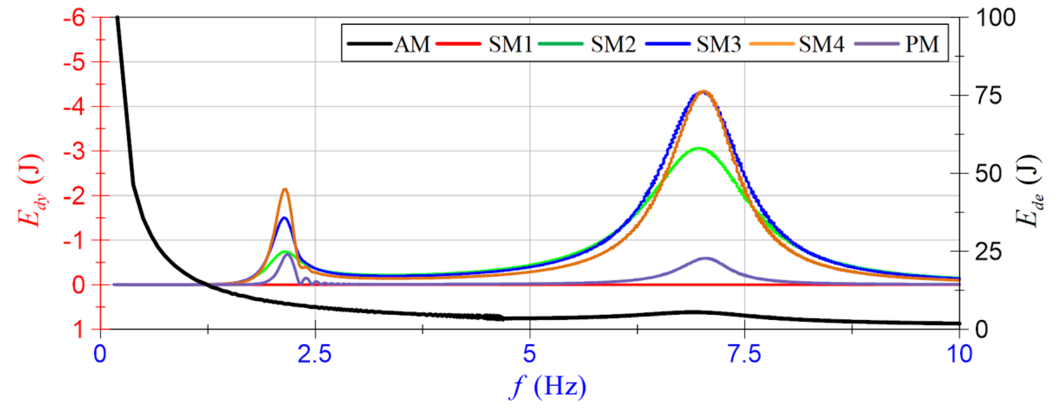
4. Simulation Tests
- Up to , SM at , increasing the amount of recovered energy;
- From to , AM in the case of available energy from an external source or SM at when no external source is available, reducing the values of and ;
- From to , SM at , value reduction and increase the amount of recovered energy;
- From to , SM at , value reduction of ;
- Ranging from , SM at , value reduction of , increasing the amount of recovered energy.
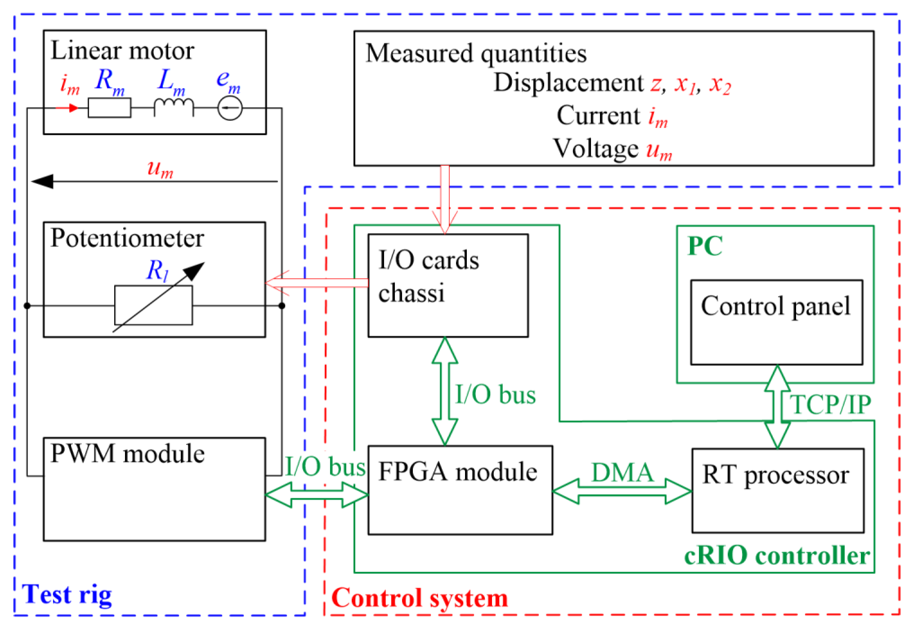
5. Experimental Tests
6. Conclusions
Author Contributions
Funding
Conflicts of Interest
References
- Korenev, B.G.; Reznikov, L.M. Dynamic Vibration Absorbers: Theory and Technical Applications; Wiley: Chichester, UK; New York, NY, USA, 1993; ISBN 978-0-471-92850-8. [Google Scholar]
- Sykes, A.O. Isolation of Vibration When Machine and Foundation Are Resilient and When Wave Effects Occur in the Mount. Noise Control 1960, 6, 23–38. [Google Scholar] [CrossRef]
- Van de Vegte, J.; de Silva, C.W. Design of Passive Vibration Controls for Internally Damped Beams by Modal Control Techniques. J. Sound Vib. 1976, 45, 417–425. [Google Scholar] [CrossRef]
- Lo Feudo, S.; Touzé, C.; Boisson, J.; Cumunel, G. Nonlinear Magnetic Vibration Absorber for Passive Control of a Multi–Storey Structure. J. Sound Vib. 2019, 438, 33–53. [Google Scholar] [CrossRef] [Green Version]
- Balaji, P.S.; Karthik SelvaKumar, K. Applications of Nonlinearity in Passive Vibration Control: A Review. J. Vib. Eng. Technol. 2021, 9, 183–213. [Google Scholar] [CrossRef]
- Rockwell, T.H.; Lawther, J.M. Theoretical and Experimental Results on Active Vibration Dampers. J. Acoust. Soc. Am. 1962, 34, 1976. [Google Scholar] [CrossRef]
- Preumont, A.; Seto, K. Active Control of Structures; John Wiley: Chichester, UK, 2008; ISBN 978-0-470-03393-7. [Google Scholar]
- Jungblut, J.; Fischer, C.; Rinderknecht, S. Active Vibration Control of a Gyroscopic Rotor Using Experimental Modal Analysis. Bull. Pol. Acad. Sci. Tech. Sci. 2021, 69, e138090. [Google Scholar]
- Verma, M.; Collette, C. Active Vibration Isolation System for Drone Cameras. In Proceedings of the 14th International Conference on Vibration Problems; Sapountzakis, E.J., Banerjee, M., Biswas, P., Inan, E., Eds.; Lecture Notes in Mechanical Engineering. Springer: Singapore, 2021; pp. 1067–1084, ISBN 9789811580482. [Google Scholar]
- Yuan, L.; Sun, S.; Pan, Z.; Ding, D.; Gienke, O.; Li, W. Mode Coupling Chatter Suppression for Robotic Machining Using Semi-Active Magnetorheological Elastomers Absorber. Mech. Syst. Signal Processing 2019, 117, 221–237. [Google Scholar] [CrossRef]
- Yang, J.; Ning, D.; Sun, S.S.; Zheng, J.; Lu, H.; Nakano, M.; Zhang, S.; Du, H.; Li, W.H. A Semi-Active Suspension Using a Magnetorheological Damper with Nonlinear Negative-Stiffness Component. Mech. Syst. Signal Processing 2021, 147, 107071. [Google Scholar] [CrossRef]
- Min, C.; Dahlmann, M.; Sattel, T. Numerical and Experimental Investigation of a Semi-Active Vibration Control System by Means of Vibration Energy Conversion. Energies 2021, 14, 5177. [Google Scholar] [CrossRef]
- Nerubenko, G. Vibration Energy Harvesting Damper in Vehicle Suspension. SAE Tech. Pap. 2020. [Google Scholar] [CrossRef]
- Sapiński, B. Experimental Study of a Self-Powered and Sensing MR-Damper-Based Vibration Control System. Smart Mater. Struct. 2011, 20, 105007. [Google Scholar] [CrossRef]
- Sapiński, B.; Orkisz, P.; Jastrzębski, Ł. Experimental Analysis of Power Flows in the Regenerative Vibration Reduction System with a Magnetorheological Damper. Energies 2021, 14, 848. [Google Scholar] [CrossRef]
- Yang, Y.; Zhao, X.; Shi, W.-X. Hybrid Application of Tuned and Viscous Dampers for Improving Human Comfort Performance of Super Tall Buildings. In Proceedings of the Mechanics and Materials Science; WORLD SCIENTIFIC: Guangzhou, China, 2017; pp. 1071–1078. [Google Scholar]
- Rahmat, M.S.; Hudha, K.; Abd Kadir, Z.; Amer, N.H.; Mohamad Nor, N.; Choi, S.B. A Hybrid Skyhook Active Force Control for Impact Mitigation Using Magneto-Rheological Elastomer Isolator. Smart Mater. Struct. 2021, 30, 025043. [Google Scholar] [CrossRef]
- Busby, H.R.; Staab, G.H. Structural Dynamics: Concepts and Applications; CRC Press: Boca Raton, FL, USA, 2017; ISBN 1-4987-6597-1. [Google Scholar]
- Rajamani, R. Vehicle Dynamics and Control; Springer Science & Business Media: Berlin/Heidelberg, Germany, 2011; ISBN 1-4614-1432-6. [Google Scholar]
- Deshpande, V.S.; Mohan, B.; Shendge, P.D.; Phadke, S.B. Disturbance Observer Based Sliding Mode Control of Active Suspension Systems. J. Sound Vib. 2014, 333, 2281–2296. [Google Scholar] [CrossRef]
- Strecker, Z.; Mazůrek, I.; Roupec, J.; Klapka, M. Influence of MR Damper Response Time on Semiactive Suspension Control Efficiency. Meccanica 2015, 50, 1949–1959. [Google Scholar] [CrossRef]
- Elias, S.; Matsagar, V. Research Developments in Vibration Control of Structures Using Passive Tuned Mass Dampers. Annu. Rev. Control 2017, 44, 129–156. [Google Scholar] [CrossRef]
- Tesfay, A.H.; Goel, V.K. Analysis of Semi-Active Vehicle Suspension System Using Airspring and MR Damper. IOP Conf. Ser. Mater. Sci. Eng. 2015, 100, 012020. [Google Scholar] [CrossRef]
- Oliveira, K.F.; César, M.B.; Gonçalves, J. Fuzzy Based Control of a Vehicle Suspension System Using a MR Damper. In CONTROLO 2016; Garrido, P., Soares, F., Moreira, A.P., Eds.; Lecture Notes in Electrical Engineering; Springer International Publishing: Cham, Switzerland, 2017; Volume 402, pp. 571–581. ISBN 978-3-319-43670-8. [Google Scholar]
- Le, T.D.; Ahn, K.K. A Vibration Isolation System in Low Frequency Excitation Region Using Negative Stiffness Structure for Vehicle Seat. J. Sound Vib. 2011, 330, 6311–6335. [Google Scholar] [CrossRef]
- Utkin, V.I. Sliding Modes in Control and Optimisation; Springer Science & Business Media: Berlin/Heidelberg, Germany, 2013; ISBN 3-642-84379-4. [Google Scholar]
- Davila, J.; Fridman, L.; Levant, A. Second-Order Sliding-Mode Observer for Mechanical Systems. IEEE Trans. Automat. Contr. 2005, 50, 1785–1789. [Google Scholar] [CrossRef]
- Linear Actuator, LA25-42-000A, Technical Documentation. Available online: https://www.sensata.com/sites/default/files/a/sensata-linear-actuator-LA-25-42-drawing.pdf (accessed on 21 October 2021).
- Linear Actuator, LA30-43-000A, Technical Documentation. Available online: https://www.sensata.com/sites/default/files/a/sensata-voice-coil-actuator-linear-frameless-la30-43-000a-drawing.pdf (accessed on 21 October 2021).
- Linear Encoder with Integrated Converter, LIKA SMK, Technical Documentation. Available online: http://www.lika.pl/pliki_do_pobrania/CAT%20SMK%20E.pdf (accessed on 21 October 2021).
- Linear Encoder with Sinus/Cosinus Output, LIKA SMS12, Technical Documentation. Available online: http://www.lika.pl/pliki_do_pobrania/CAT%20SMS12%20E.pdf (accessed on 21 October 2021).
- Shtessel, Y.; Edwards, C.; Fridman, L.; Levant, A. Sliding Mode Control and Observation; Springer: Berlin/Heidelberg, Germany, 2014. [Google Scholar]
- Bacciotti, A.; Rosier, L. Liapunov Functions and Stability in Control Theory; Springer Science & Business Media: Berlin/Heidelberg, Germany, 2005; ISBN 3-540-21332-5. [Google Scholar]
- Snamina, J.; Orkisz, P. Active Vibration Reduction System with Mass Damper Tuned Using the Sliding Mode Control Algorithm. J. Low Freq. Noise Vib. Act. Control 2021, 40, 540–554. [Google Scholar] [CrossRef] [Green Version]
- Zhang, W. Quantitative Process Control Theory; CRC Press: Boca Raton, FL, USA, 2011; Volume 45, ISBN 1-4398-5561-7. [Google Scholar]
- CompactRIO Controller, Technical Documentation. Available online: https://www.ni.com/pl-pl/support/model.crio-9063.html (accessed on 21 October 2021).
- NI 9505 PWM Module, Technical Documentation. Available online: https://www.ni.com/pdf/manuals/374211h.pdf (accessed on 21 October 2021).


| Symbol | Description | Symbol | Description |
|---|---|---|---|
| time | sliding variable | ||
| simulation time | angle of the sliding surface on a state trajectory | ||
| displacement of shaker plate | Lyapunov function | ||
| displacement of plate 1 | |||
| displacement of plate 2 | |||
| mass of plate 1 | |||
| mass of plate 2 | |||
| damping coefficient | |||
| damping coefficient | frequency of the input signal | ||
| spring coefficient | starting frequency | ||
| spring coefficient | ending frequency | ||
| motor control force | |||
| force sensitivity coefficient | |||
| back emf coefficient | |||
| electromotive force | displacement transmissibility | ||
| motor resistance | displacement transmissibility | ||
| motor inductance | |||
| current in motor circuit | |||
| motor circuit voltage | dynamic performance coefficient | ||
| additional resistance | -th displacement cycle | ||
| equivalent damping coefficient | dissipated energy in the time duration of one cycle of displacement | ||
| control force | delivered energy in the time duration of one cycle of displacement | ||
| disturbing force | energy consumption coefficient |
| Mechanical Parameters | |||||
| Electrical Parameters | |||||
| Mode | ||||||
|---|---|---|---|---|---|---|
| PM | 79.3 | 103.7 | 19.69 | 33.55 | 4.25 | −0.67 |
| SM1 | 56.8 | 76.3 | 2.02 | 2.94 | 61.97 | 0 |
| SM2 | 59.2 | 77.2 | 2.97 | 4.74 | 58.60 | −0.74 |
| SM3 | 66.5 | 86.5 | 4.36 | 7.23 | 50.83 | −1.49 |
| SM4 | 71.6 | 93.1 | 6.35 | 10.7 | 42.79 | −2.14 |
| AM | 43.5 | 45.1 | 0.75 | 0.70 | 76.38 | 8.11 |
| Semi-Active Mode | ||||
| I | ||||
| II | ||||
| III | ||||
| Hybrid Mode | ||||
| I | ||||
| II | ||||
| III | ||||
| IV | ||||
| V | ||||
Publisher’s Note: MDPI stays neutral with regard to jurisdictional claims in published maps and institutional affiliations. |
© 2022 by the authors. Licensee MDPI, Basel, Switzerland. This article is an open access article distributed under the terms and conditions of the Creative Commons Attribution (CC BY) license (https://creativecommons.org/licenses/by/4.0/).
Share and Cite
Orkisz, P.; Sapiński, B. Vibration Reduction System with a Linear Motor: Operation Modes, Dynamic Performance, Energy Consumption. Energies 2022, 15, 1910. https://doi.org/10.3390/en15051910
Orkisz P, Sapiński B. Vibration Reduction System with a Linear Motor: Operation Modes, Dynamic Performance, Energy Consumption. Energies. 2022; 15(5):1910. https://doi.org/10.3390/en15051910
Chicago/Turabian StyleOrkisz, Paweł, and Bogdan Sapiński. 2022. "Vibration Reduction System with a Linear Motor: Operation Modes, Dynamic Performance, Energy Consumption" Energies 15, no. 5: 1910. https://doi.org/10.3390/en15051910
APA StyleOrkisz, P., & Sapiński, B. (2022). Vibration Reduction System with a Linear Motor: Operation Modes, Dynamic Performance, Energy Consumption. Energies, 15(5), 1910. https://doi.org/10.3390/en15051910