Proposal of Multidimensional Data Driven Decomposition Method for Fault Identification of Large Turbomachinery

Abstract

High-power turbomachines are equipped with flexible rotors and journal bearings and operate above their first and sometimes even second critical speed. The transient response of such a system is complex but can provide valuable information about the dynamic state and potential malfunctions. However, due to the high complexity of the signal and the nonlinearity of the system response, the analysis of transients is a highly complex process that requires expert knowledge in diagnostics, machine dynamics, and extensive experience. The article proposes the Multidimensional Data Driven Decomposition (MD3) method, which allows decomposing a complex transient into several simpler, easier to analyze functions. These functions have physical meaning. Thus, the method belongs to the Explainable Artificial Intelligence area. The MD3 method proposes three scenarios and chooses the best based on the MSE quality index. The approach was first verified on a test rig and then validated on data from a real object. The results confirm the correctness of the method assumptions and performance. Furthermore, the MD3 method successfully identified the failure of rotor unbalance, both on the test rig and the real object data (large generator rotor in the power plant). Finally, further directions for research and development of the method are proposed.

1. Introduction

Electrical energy plays a vital role in all branches of industry. This form of energy can be utilized in different ways and formats. This versatility makes it the very foundation of modern industry and society. Although renewable energy each year takes a bigger and bigger share in the power generation market, the power supply safety system requires large units to exist. Another important use of steam plants is suppling steam required by numerous industrial plants (e.g., chemical or paper plants). In such cases, renewal energy fails to provide such media as was depicted in the report [1]. The overwhelming majority of steam used in industry branches and electrical power comes from steam turbogenerator sets. Their architecture and operation are very complex. Therefore, the diagnostic process of such equipment is far from trivial. Often these units are critical to the process. Therefore, they are well-instrumented in monitoring their technical state, but plants often lack qualified personnel on-site to correctly and precisely diagnose any potential malfunctions. Diagnostics of large turbomachinery uses data in transient states (during start-ups and coast downs), especially for detecting and identifying malfunctions at the early stages of fault development. Missing a fault may lead to unplanned outages and generate substantial additional costs making the enterprise less profitable. In extreme cases, poorly monitored and badly diagnosed units can suffer from catastrophic failures and damage the whole power plant. In this case, the rebuilding of the unit is necessary. The collective work [2] depicts the failures of machines without proper diagnosis. This research aims to help the operation and maintenance staff diagnose the primary failure modes properly. The authors in this paper focus on the automatic analysis of transient states (coast-downs and start-ups). These states are often overlooked but contain essential information about the technical condition of rotating machines. Although the field of vibration research is vast, the authors noticed a lack of automatic methods that would determine the dynamic parameters of turbine sets during a transient state.

The new paradigm of Industry 4.0 is also introduced to large turbomachinery. New condition monitoring strategies for these machines were well described by Jabłoński and Barszcz in [3] and Capelli et al. [4]. This new approach requires new ways of monitoring the turbines. Banaszkiewicz in [5] showed a concept lifetime assessment system for steam turbines that considers a wide range of operating condition changes in the scope of creep-fatigue damage. Zagorowska et al. [6] presented an interesting concept of exponential trend approximation with shape adaptation to monitor performance degradation during operation. Hanachi et al. [7] presented an interesting approach to improving prognostic accuracy in the compressor section of gas turbines by taking into account the effects of humidity, and Zohair et al. [8] proposed a modified Weibull distribution as a reliability estimator for gas compression turbines to reduce the failure risk. These works are of great value and present an improved way of monitoring the rotating machines; however, they are missing much information on machine dynamic conditions. This information comes from a transient state of the turbogenerator

Turbogenerators are equipped with fluid-film sliding journal bearings, which are very well described and examined in the first chapter of [9] and throughout [10]. Figure 1a depicts the schematics of the eddy-current arrangement in the bearing housing, and Figure 1b depicts the real assembly of these sensors. Turbogenerators’ rotors operate above the first, second, and even third of their bending mode. Bently and Hatch in [11] (Chapter 12) described modes of vibration and rotor shapes in detail. Critical speed calculations and particular shapes of the rotor while passing through these critical rotational speed intervals were extensively studied and well described by Muszyńska in [12], Ehrich in [13], Vance in [14], and Kiciński in [15]. The behavior of this type of equipment is highly nonlinear. Thus, it is nearly impossible to properly diagnose it without an expert’s knowledge backed by extensive experience in bearings and rotordynamics analysis. Difficulties in transient state analysis are complex but bring many benefits. As Eisenmann pointed out and proved with a lot of examples in his book [16], many malfunctions can be diagnosed based on the analysis of the transient response of a rotor-bearing system. The works of [11,12,13,14] describe the most common malfunctions and diagnostic procedures to determine them. Malfunctions that can be determined on the base of their transient vibration signature are:

• Unbalance;
• Resonance;
• Misalignment;
• Rub;
• Hydrodynamic instability (oil whirl/whip).

Akhtar et al. in [17] presented the reality and the amount of work and tools necessary to diagnose a gas turbine that experienced high vibration amplitudes properly. Knowledge of a particular failure mode can benefit both operational staff and the management. The first will benefit from operating the machine more safely and reliably. The latter will be able to plan the overhauls precisely and make the production more sustainable while lowering the production costs and maximizing the benefits. Brito et al. in [18] present several advancements in fault detection, diagnosis, and prognosis in rotating machinery. From this perspective, automatic detection of common malfunctions can become an exciting complement to standard monitoring equipment.

Several researchers investigated the model-based approach, also referred to as the “white box”. For example, Xia et al. in [19] described an interesting approach to identifying sudden unbalance changes in the speed-varying rotor during start-up. In his research, he used the Finite Element (FE) model of a test rig that can become very complex when considering the whole turbogenerator set. Kiciński, in his books [10] and [15], presented the development of FE models of the 13K215 type of the turbogenerator set. The complexity of such an approach can also be seen in the work by Adams [20], who in his book described analyses, diagnoses, and troubleshoots for different types of flexible rotors, taking into account FE models of rotor and rotor-to-bearing. Although precise, this approach to the problem quickly becomes too complex to implement in an online approach and produce any reliable conclusions, especially without an expert on-site.

As was stated by Fu et al. [21], the transient state of a machine is a rich source of valuable diagnostic data, especially when it comes to unbalance response in a hollow-shaft overhung rotor. Comparison and proper assessment of the data must consider the rotational speed. Several works describe the advantages of this kind of analysis, for example, books by Wowk [22] and Ehrich [13]. Bornassi et al. in [23] showed an interesting approach to identifying rotor-blades parameters undergoing non-stationary conditions. Zhou et al. [24] described a time series analysis that handled non-stationary, nonlinear inputs using signal decomposition. He argues that the empirical Fourier decomposition method can decompose signals more accurately than the empirical wavelet transform. Nishat Toma and Kim in [25] used a classification scheme and the current discrete wavelet transform to extract diagnostic features for the induction motor.

The “intelligent” methods only consider steady-state operations in which the diagnostic patterns will appear. Brito et al. in [18] showed advantages in unsupervised learning and its incorporation in rotating machinery fault pattern detection and diagnosis. It constitutes a methodology to detect a fault mode and predict its trend. In fault diagnosis, he used the black-box model approach and the Shapely Additive Explanations method. He used unsupervised classification and root cause analysis to produce a diagnosis. Zhang et al. in [26,27] presented an interesting approach to “the next level” of data driven machinery diagnostics. He proposed a method that joins the domain gap across varying operating conditions. Although his work implies effective applications for the rolling element bearings in the train industry, it can produce proper cross-domain fault diagnosis only with a balanced amount of different fault modes data available. In large turbomachinery, this is not the case. The fault mode data are not often found. Furthermore, there is no available training data set due to the low rate of transient states during the machine’s lifetime (and even less with a fault). Additionally, a few state-of-the-art anomaly detection algorithms are examined. Thus, there is a shortage of techniques dealing with the transient states, especially for large turbogenerators, for which the transient data sets become very large both in terms of data points and in terms of time.

The authors in [28] proposed foundations and the basic considerations of automated turbomachinery fault identification. The concept was presented for one channel only with unprocessed data and without any severe malfunctions. For such a trivial case, one probe is quite useful and sufficient. However, taking into account the whole turbogenerator shaftline relying on a single sensor at a time often lacks essential information. Furthermore, different malfunctions can be revealed in different stages of the machine during different circumstances. Therefore, for large turbogenerator sets, multichannel analysis is a necessity. Analysis can contain different features from the same sensor (e.g., overall vibration amplitude, its first harmonic and phase, second harmonic, subharmonics, and others). Additionally, the investigation can incorporate different sensors from the same bearing (the orthogonally oriented in the bearing plane). Finally, the research can use sensors at different axial locations along the shaftline. The above-described analysis challenges are why the original method, proposed in [28] for a single sensor, must be extended to a multidimensional case.

The main goal of our work was the research of an autonomous method to diagnose large rotating equipment. Some works heading in the same direction were published in recent years. For instance, Bielecki et al. in [29] proposed a simple yet effective method for unsupervised monitoring of rotating machinery for failure detection in the early stages. Lei et al. in [30] incorporated unsupervised feature learning on a big data set to diagnose the motor and locomotive bearing faults patterns. All these works consider machines during their steady-state operation. There is a lack of work that take into account the transient states of large turbomachinery.

Wang and Sun [31] used the combination of wavelet decomposition sparse filtering networks and a support vector machine to establish fault diagnosis in the motor bearings. Authors adopted the decomposition concept in their research.

In this paper, the authors propose the Multidimensional Data Drive Decomposition (abbreviated as MDDD or MD3), which extends the concept of transient decomposition proposed in [28] to a multichannel case. The channels are eddy-current probes mounted on the unit’s bearings or some of its parts.

The paper is structured as follows. Section 2 describes the concepts behind the method of transient decomposition. It also introduces the MD3 method and describes the complexities and challenges which caused the method to become multidimensional. Section 3 is a discussion of an optimization of the decomposed model. It describes three types of a model based on experimental and real-object data combined with the authors’ experience. The authors use Mean Squares Error (MSE) parameter for the optimization process. The outcomes of the method are summarized. A few additional concepts and signals-to-models relations which can facilitate analysis and diagnosis are described. In Section 4, validation of a model based on experimental data (measured on a test rig) is presented. The test rotor rig is prepared to exhibit the malfunction with an imbalance and the balance response. Section 5 describes a case study based on a real data example of a large turboset generator’s rotor NDE part imbalance. Finally, Section 6 contains conclusions based on our findings.

2. Method Description

Multidimensional Data Driven Decomposition (MD3) is an extension of a concept presented by the authors in [28]. This method consists of two main parts listed below:

• Real data preparation and preprocessing;
• Identification of decomposed function parameters.

The first step is required to transform very different data sets into unified vectors, which can be a subject of comparison. The content of data sets measured on the physical objects is often different. Each transient can vary depending on a large number of external factors, which are not recorded in the vibration response of the system. For instance, there can be process-dependent conditions, e.g., a low-quality vacuum in the condenser, which can cause a machine to stop much quicker than during a normal coast-down. In addition, there are transients when the Full Speed No Load (FSNL) state cannot be achieved during the start-up. There are no turbine-related issues (common ones are vacuum-related problems, lube oil-related problems, boiler-related issues, or others.). Even if the whole rpm span transient is recorded, it is evident that the vibration data are not stored at the same rotational speed instances.

Each monitoring and acquisition system records data with different resolutions in terms of time and rotational speed intervals. It is a result of the design of monitoring systems used in the field, and numerous datasets have such a feature. This data already exists, and it is not possible to repeat these measurements. Portable measurement system configuration has two different triggering options, according to the change of speed and time. Typical values are 20–60 s for time intervals and 5–50 rpm for the rotational speed change. Depending on the trip time instance, the measurement systems record the transient process at different points in time and speed. Therefore, direct comparison of the transient vibration parameters in an automated way is not possible.

As a first step, the vibration data need to be preprocessed to have the same set of rpm values. A cubic spline interpolation was introduced as the preprocessing procedure to solve this problem. It allows defining a set of equally spaced rotational speed values at which the vibration values shall be interpolated. Later, the fitness functions of the decomposed functions will be evaluated. Barszcz and Zabaryłło [32] described the usage of cubic spline interpolation and its benefits in transient state analysis. Dyer and Dyer [33] and by Schumaker [34] presented the advantage of using the equally spaced knots for the polynomial spline function (i.e., equally spaced rotational speed increments during transient). De Boor, in his book [35] in chapter XIV showed that the advantage of cubic spline interpolation is to smooth the interpolation function in the points of interest. In our research, the points of interest at which the cubic spline is calculated are the rotational speed instances from the following set $\left\{rp{m}_1,rp{m}_2,rp{m}_3,\dots ,rp{m}_{max}\right\}$. Typically, the set consists of equidistant values, e.g., 200 rpm ending at 3,000 rpm (for European power plants) with a 50 rpm distance between points.

The second step of the procedure decomposes a preprocessed transient into essential components. Finally, the procedure relates a set of function parameters and coefficients to physical phenomena occurring during the coast-downs and start-ups across the shaft line when a fault is present. Thus, the input transients are decomposed into more straightforward base functions. These functions are used as a measure of particular malfunction. Based on experience and research, the authors took a set of three decomposition base functions into account:

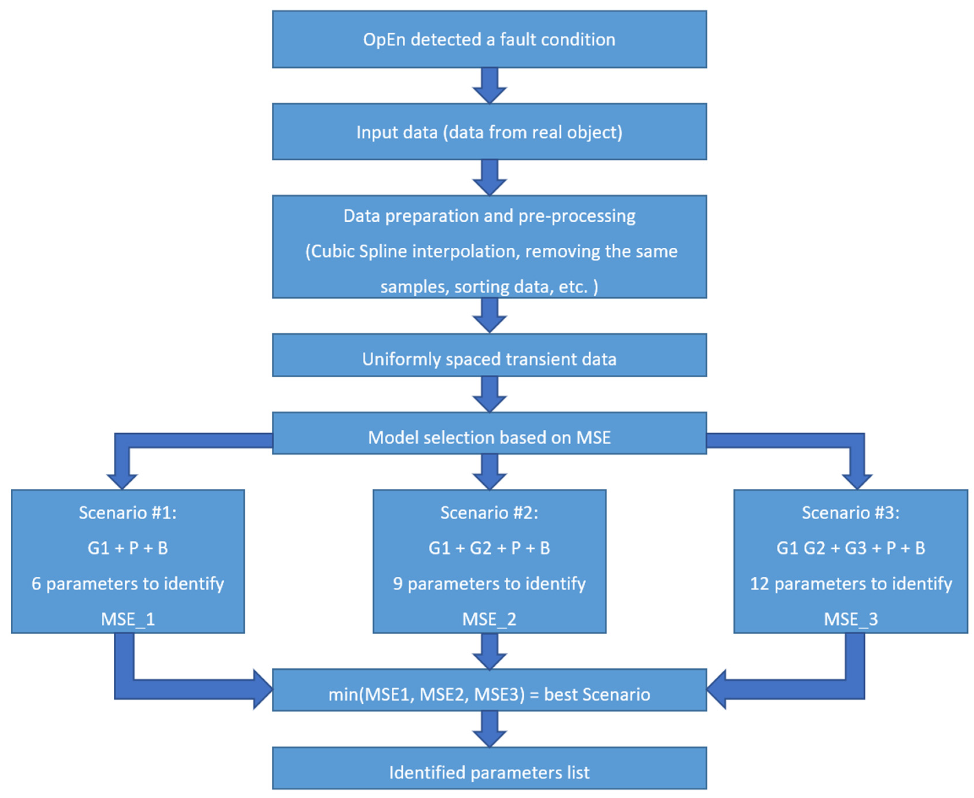
• One Gaussian function, one parabola, and one constant/bias function. It produces a set of six parameters. This scenario can identify one critical speed and unbalance.
• Two Gaussian functions are considered, one parabola and one constant/bias function. It produces a set of nine parameters. This scenario can identify rotors with two critical speed zones and unbalance.
• Three Gaussian functions are considered, one parabola and one constant/bias function. This scenario can identify rotors with up to three critical speed zones and unbalance.

Each scenario is qualified based on that same quality performance parameter, namely MSE. Mean Squared Error (MSE) measures the fitness function to be minimalized. Equation (1) presents the definition of MSE, as defined by Leon-Garcia in chapter 4 in [36].

Figure 2 presents the flow of the MD3 method divided into particular operations.

The first four blocks refer to step 1, as described at the beginning of the section. The MD3 method starts with detecting an anomaly in the OpEn procedure. After detecting a potential malfunction, the data in a set of features for individual rotational speed increments are passed for preprocessing. There are several steps in the newly received data preprocessing procedure. The first step is to sort the data samples according to the rotational speed value. This step is essential when there are different transient conditions configured. For example, during coast-down, the recording of the rotational speed would start at the highest one. The situation reverses when the start-up is recorded, and the rotational speed will start at 0 rpm. The procedure sorts the data in ascending order to rotational speed values to analyze the data systematically. Next, the samples with the same rotational speed tags are removed from the dataset. Further on, the speed range for the currently analyzed transient is determined, and the range is divided into equidistant points on the rotational speed axis. The Cubic Spline interpolation establishes equidistant points from the current transient as the last operation in this step.

The latter operations in Figure 2 belong to the second step. For each transient, three scenarios are evaluated based on the MSE quality index. First, the scenario with the best-decomposed functions fitting parameters, i.e., the smallest value of the MSE index, is chosen to represent the current transient state. These parameters can be used in malfunction identification, and they are stored for future reference.

Estimating the values of the proposed functions is the heart of the method. The authors use the Differential Evolution (DE) algorithm to determine these parameters. The algorithm finds the best fit of the assumed model vs. real-object data. Equation (2) presents how the decomposed functions are combined to form the final transient function. Finally, Equations (3)–(5) present the analytical representation of individual decomposed functions.

$$MS{E}_{trans}={{\displaystyle \sum }}_{k=1}^{rp{m}_{max}}{\left[{\phi }_{real}\left(rp{m}_k\right)-{\phi }_i\left(rpm\right)\right]}^2,$$

(1)

$${\phi }_i\left(rpm\right)={\displaystyle \sum }_{j=1}^{n}Gaus{s}_{i,j}\left(rp{m}_k\right)+P_i\left(rp{m}_k\right)+B_i\left(rp{m}_k\right),$$

(2)

$$Gaus{s}_{i,j}\left(rpm\right)=a_g{}_j{e}^{\left(-\frac{{\left(rp{m}_k-p_g{}_j\right)}^2}{2w_g{}^2}\right)},$$

(3)

$$P_i\left(rpm\right)=a_p{}_i{\left(\frac{rp{m}_k-x_p}{rp{m}_{max}-x_p}\right)}^2,$$

(4)

$$B_i=cons{t}_b,$$

(5)

where:

• $MSE$—Mean Square Error of the fitted function in particular evolution;
• $rp{m}_k$—particular rotational speed from equally spaced rotational speed increment set where $rp{m}_k ϵ \left\{rp{m}_1, rp{m}_2, rp{m}_3,\dots , rp{m}_{max}\right\}$;
• $rp{m}_{max}$—maximum rotational speed in the transient set;
• ${\phi }_{real}$—cubic spline interpolation of real data in ω instances;
• ${\phi }_i$—cubic spline interpolation of real data in ω instances;
• $n$—a number of Gaussian functions chosen for the decomposition;
• $j ϵ \left\{1,2,3,\dots , n\right\}$—particular Gaussian function in $n$ set;
• $Gaus{s}_{i,j}\left(rpm\right)—j$-th Gaussian function;
• $P_i$—parabola function (2nd-degree polynomial);
• $B_i$—bias function with its parameter (constant not dependent on $rpm$);
• $a_g{}_j$—amplitude of $j$-th Gaussian function at the top of its critical speed (resonant speed);
• $p_g{}_j$—the peak of the $j$-th Gaussian function in terms of rotational speed;
• $w_g{}_j$—width of the resonant zone of the $j$-th Gaussian function;
• $a_p{}_i$—amplitude of $i$-th parabola function at the end of the recorded transient;
• $x_p$—point of start of the parabola in terms of rotational speed ($rpm$);
• $cons{t}_b$—constant term taking into account initial vibration indication of the shaft.

Figure 3 presents an example of the nonlinearity of the system during transience. The upper plot presents the phase of vibration, and the lower plot presents the vibration amplitude. The X-axis represents rotational speed. Highly nonlinear system responses during transient states can cause analytical methods to be hard to implement. The analysis outcome might not be fully comprehensible for a non-expert. Examples of the rotor-bearing system analytical model complexity can be found in [12] by Muszyńska and in [10] and by Kiciński [15]. Such complexity, in most cases, causes the machinery users not to use the analytical methods. To facilitate the rotating systems analysis, the authors proposed in [28] a proposal to decompose the turbo-set transient data into several more straightforward to analyze signals. The signals’ decomposition was successfully developed and implemented for a single sensor from a large turbogenerator.

The results depicted in [28] include transient signal data from one sensor only. Its results were promising, and it validated the concept of decomposition, and the parameters of decomposed functions did have a mechanical meaning. However, further improvement of the method is necessary. The available data are much richer than only a single 1X parameter of a single vibration sensor, where 1X means an amplitude of a synchronous response of the rotor in one bearing and in one plane (depicted in Figure 3 in the lower plot by the red line). First, many sensors are installed (typically, two eddy-current vibration sensors per one bearing). Second, a set of features is calculated from each sensor. Figure 4 presents a tabular list of the features calculated by the portable measuring equipment during the measurement course. The most important features for diagnostic purposes are:

• Overall vibration amplitude (column called Direct);
• The amplitude of the first harmonic of the signal (column called 1X_Amplitude);
• The phase angle of the first harmonic (column called 1X_Phase);
• The amplitude of the second harmonic of the signal (column called 2X_Amplitude);
• The phase angle of the second harmonic (column called 2X_Phase);
• The amplitude of the sub-harmonic of the signal (column called nX_Amplitude);
• The phase angle of the sub-harmonic (column called nX_Phase).

Figure 4 depicts three time instances during the transient measurement process. The top part presents the data on FSNL. The middle one shows the data at approximately 2700 rpm. Finally, the bottom one depicts the data at approximately 1100 rpm. One can note that data on specific time instances during the transient are extremely different (e.g., in row 2Y-Ch# 3, the Direct value is 32, 100, 200 µm_pp on FSNL, 2700, and 1100 rpm, respectively).

Thus, for a medium-size turbo generator with 7 bearings, the number of transients to analyze can easily reach 20–50 transient data sets. Data from different sensors installed along the shaftline are very different depending on the placement of the sensor location. Data are significantly different for a 200 MW equipped with a 7 bearings machine. Near FSNL operation, the second harmonic amplitude can be apparent and even dominant at the generator bearings. It is a typical vibration pattern observed in large turbogenerators, and such behavior does not imply operational issues or malfunctions. On the other hand, high values of the second harmonic amplitude between IP and LP (Low Pressure) parts can be a symptom of misalignment.

On the other hand, in some cases, if there is an unbalance on the shaft line, the data patterns from different sensors will be similar. Consequently, the synchronous response of the imbalanced rotor will eventually have the same form of vibration dependency on rotational speed (described by Equation (4)) for every sensor. However, the function parameters will be quite different. In other cases, if a journal bearing supporting shaft develops an oil whirl or whip, it will cause a rapid increase in the direct and sub-synchronous response.

So, it is clear that real fault identification requires a multidimensional approach. Only such an approach will help to diagnose particular malfunction patterns more accurately. For example, the synchronous amplitude and phase have to be taken into account to diagnose the unbalance properly. In a simple case like static unbalance, one sensor may be sufficient to produce a proper diagnosis, though another sensor should verify it at the other end of the same shaft. In a more complex case of a dynamic unbalance, the situation has to be analyzed in at least two planes with two sensors at each plane and in the same angular orientation. This procedure requires at least two sensors with two features.

The complexity of inter-dependencies and the computational time for data analysis makes this challenging. Analyzing all the sensors and their features at once turns out to be not practical. After some research, we propose that it is reasonable to analyze data from at least two bearings from the same shaft.

The authors used the Differential Evolution algorithm to automate the function parameters decomposition process. The DE algorithm is part of the Genetic Algorithms (GA) family. Genetic Algorithms are based on the concept of population evolution in a natural habitat. The idea of finding the best solution to a given problem (goal function) was described by Koza and Poli in Chapter 5 [37]. Finding the solution starts with some initial set of solutions with different parameters (called population) and using the quality parameter (called fitness function) to determine the best solutions from the solutions’ pool (the fittest individuals from the particular population, called parents). Then, another set of solutions based on the parents (called children) is produced. Children inherit many properties from their parents, but they can also be subjected to modifications in their parameters (called mutation and genes’ crossover). Then, the new solution set of the next evolution is ready to be evaluated. This can go on until the quality parameter is met or for an arbitrary amount of evolutions.

GA algorithms are used extensively across many fields of science and engineering. For example, Roetzel et al., in chapter 6 in [38], described the heat exchanger networks design using GA with network parameters like Total Annual Cost, target temperatures hot and cold temperatures with good results. Furthermore, Li et al. in [39] argued that GA feature optimization and Back Propagation Neural Networks could be applied in cardiac arrhythmia automatic identification due to dimension reduction. It can yield a classification accuracy of 99.33%.

Storn and Price in [40] stated that DE algorithms fall into the evolutionary computing algorithms family. It became a versatile tool for finding non-differentiable nonlinear optimal solutions to multidimensional objective functions. It can be described as a metaheuristic search algorithm that uses the population-based principle to improve its finding performance in an iterative way. Throughout recent decades many improvements have been proposed in terms of DE mutation strategies [41,42], population initialization [43,44], population enhancement schemes [45], and crossover strategies [46].

The review paper by Ahmad et al. [47] described massive progress in the DE research and application fields in recent years. It evaluated different modifications of DE algorithms in terms of search accuracy and efficiency. It analyzed the setting of numerous parameters to identify optimal values for problem-solving. Their flexibility in parameter constraints is used in many fields to find the optimal solution. For example, in the civil engineering domain, Georgioudakis and Plevris [48] presented the DE algorithm as a great tool that finds the optimum solution in constrained structural optimization. In hydrokinetic turbine design, Muratoglu et al. [49] introduced the DE algorithm to optimize the turbine’s blade sections with multidimensional design objectives. It includes high hydrodynamic forces, cavitation, leading-edge contamination, and ideal stall behavior. Li et al. in [50] used DE to extract parameters of photovoltaic models based on current-voltage measurements. On the other hand, Mustafi and Sahoo [51] used it in cooperation with the GA algorithm to find the best parameters of centroids used by the k-means clustering algorithm to avoid its convergence to local optimum in the text document clustering task.

The authors in [28] have successfully implemented the DE algorithm to automatically find 11 parameters of 4 decomposed functions on 2 reference data sets. One data feed to the DE algorithm came as baseline data with no known malfunctions, and the second one was with a misalignment fault pattern. These transients were decomposed, and the results were exciting and promising for further investigation.

The Data Driven Decomposition (D3) method was developed by the authors in [28]. It uses a single sensor and single feature, i.e., the analysis and identification are one-dimensional. As presented earlier in this section, relying on a single sensor for complete diagnostics of a large machine is not sufficient. Data from more sensors and features should be analyzed together to obtain more accurate fault identification. Such a necessity determines the introduction of another level of dimensionality. Multidimensionality concerns the number of sensors used for the analysis and the analyzed features. This motivates the authors’ concept proposal and explains why they coined the Multidimensional Data Driven Decomposition Method. However, due to the complexity of the system response described earlier, it is not practical to analyze all the available data. Based on the authors’ experience, it was decided to identify decomposed transient function parameters and analyze the data from the two nearest bearings (or a single shaft) at the time.

3. Optimization of Decomposed Model

Barszcz and Zabaryłło described the process of anomaly detection during transient states in [32]. In that paper, they lay the Operating Envelope (OpEn) concept as a method for fault detection for transients. The method introduces a criterion of acceptance region for transient data sets and detects a possible deviation from the baseline measurements. When the transient data do not exceed OpEn upper and lower values (which may require a multidimensional approach), the measured transient is assumed to be not significantly different from the baseline. Therefore, the behavior of the machine belongs to the correct category. In other words, if the machine vibrations are contained inside the OpEn region throughout the whole transient (all the rotational speed span), it is assumed to be in a healthy state condition, and no corrective actions have to be undertaken.

On the other hand, when some data exceed the OpEn region, it is assumed that some deviations from normal behavior are present in the system, and the anomaly identification process has to be performed. This is a situation when the proposed MD3 algorithm shows its value in automatic analysis of machine health. The MD3 method’s main part is to obtain parameters of base functions, which reflect particular malfunctions. This process depends on which functions are selected as the set of base functions. Therefore, this process required optimization. The results of this research are presented in this section.

The transient data set can be very different, depending on the sensor location and the type of malfunction. To correctly identify the shape of the transient data and not fall into underestimation or overfitting, we propose to apply several sets of base functions. Therefore, a few most probable scenarios will be investigated by the GA/DE algorithm. Next, the results of all the scenarios will be compared. The best scenario will be selected based on the MSE quality measure expressed by Equation (1). Then, the scenario with the smallest MSE value will be chosen as the best fit. These sorts of considerations are valid for all of the bearings and all the rotors in the turbo-set. As the authors pointed out earlier, the data from different transducers and locations must be compared to make the diagnosis more precise. In extreme cases, a few cylinders have to be considered in the analysis process. In these cases, the amount of real-object data and time to process them grows significantly with each sensor added. To enhance the MD3 method performance of the possible space of decomposed signal function, we propose to limit the number of input sensors to a single shaft (aka. cylinder).

Next, several scenarios of base function sets were selected and compared.

Table 1. Scenarios for model selection.

Scenario	Decomposed Functions	Parameters to be Identified
1	$G_1+P+B$	$\left\{\begin{array}{c}{a}_{g_1},rp{m}_{g_1},w_{g_1},\\ a_p,x_p,\\ cons{t}_b\end{array}\right\}=6$
2	$G_1+G_2+P+B$	$\left\{\begin{array}{c}{a}_{g_1},rp{m}_{g_1},w_{g_1},a_{g_2},rp{m}_{g_2},w_{g_2},\\ a_p,x_p,\\ cons{t}_b\end{array}\right\}=9$
3	$G_1+G_2+G_3+P+B$	$\left\{\begin{array}{c}{a}_{g_1},rp{m}_{g_1},w_{g_1},a_{g_2},rp{m}_{g_2},w_{g_2},a_{g_3},rp{m}_{g_3},w_{g_3},\\ a_p,x_p,\\ cons{t}_b\end{array}\right\}=12$

presents the selected sets. Each scenario is composed of a Gaussian, parabola, and constant function described by Equations (3)–(5), respectively, in different combinations. The main differentiator is the number of resonances a shaft can reflect in the recorded data. Based on the engineering practice, we know that, in reality, the number of these resonances can vary from 1 to 3. The two remaining components are parabolic function (to reflect a possible unbalance) and a constant bias (noise vibration level). Thus, scenario 1 has the simplest form described by Equation (6). It consists of a single Gaussian function, parabola, and constant term. This scenario can detect the initial bias term introduced to a system, one critical speed zone with its parameters like the placement of a peak, its height, and the width of the zone. It can also detect a moderate unbalance response.

Equation (7) describes scenario 2. This is an extension of scenario 1 by adding another Gaussian function by which a second critical speed zone can be identified.

Scenario 3 is depicted in Equation (8), extending scenario 2 by adding the third Gaussian function to its identification capabilities. This most advanced scenario has 12 parameters of 5 decomposed functions to be identified. This can identify a third critical speed zone or additional nonlinearity.

$$Scenari{o}_1=a_g{}_1{e}^{\left(-\frac{{\left(rpm-p_g{}_1\right)}^2}{2w_g{{}_1}^2}\right)}+a_p{\left(\frac{rpm-x_p}{rp{m}_{max}-x_p}\right)}^2+cons{t}_b,$$

(6)

$$Scenari{o}_2=a_g{}_1{e}^{\left(-\frac{{\left(rpm-p_g{}_1\right)}^2}{2w_g{{}_1}^2}\right)}+a_g{}_2{e}^{\left(-\frac{{\left(rpm-p_g{}_2\right)}^2}{2w_g{{}_2}^2}\right)}+a_p{\left(\frac{rpm-x_p}{rp{m}_{max}-x_p}\right)}^2+cons{t}_b$$

(7)

$$Scenari{o}_3=a_g{}_1{e}^{\left(-\frac{{\left(rpm-p_g{}_1\right)}^2}{2w_g{{}_1}^2}\right)}+a_g{}_2{e}^{\left(-\frac{{\left(rpm-p_g{}_2\right)}^2}{2w_g{{}_2}^2}\right)}+a_g{}_3{e}^{\left(-\frac{{\left(rpm-p_g{}_3\right)}^2}{2w_g{{}_3}^2}\right)}+a_p{\left(\frac{rpm-x_p}{rp{m}_{max}-x_p}\right)}^2+cons{t}_b$$

(8)

The most advanced scenario consists of 12 parameters of 5 decomposed functions to be identified, extending scenario 2 by adding the third Gaussian function to its identification capabilities. This can identify a third critical speed zone, or additional nonlinearity can be introduced to approximate the examined system’s response. Scenario 3 functions are depicted in Equation (8).

The time required for base function parameter fitting varies significantly, depending on the DE algorithm input parameter range. Critical parameters concerning time-to-performance are the population count and count of evolution.

Table 2. Time of decomposed function parameters identification depending on DE algorithm parameters change.

Population Count	Number of Evolutions	MSE_1 Identification Time [s]	MSE_2 Identification Time [s]	MSE_3 Identification Time [s]
${\mathrm{P}}_{\mathrm{op}}=20$	$E_{vol}=200$	3	4	7
${\mathrm{P}}_{\mathrm{op}}=20$	$E_{vol}=500$	7	11	12
${\mathrm{P}}_{\mathrm{op}}=20$	$E_{vol}=1000$	13	18	21
${\mathrm{P}}_{\mathrm{op}}=30$	$E_{vol}=500$	9	13	16
${\mathrm{P}}_{\mathrm{op}}=30$	$E_{vol}=1000$	20	25	35
${\mathrm{P}}_{\mathrm{op}}=30$	$E_{vol}=2000$	31	48	60
${\mathrm{P}}_{\mathrm{op}}=40$	$E_{vol}=500$	12	19	21
${\mathrm{P}}_{\mathrm{op}}=40$	$E_{vol}=1000$	22	33	46
${\mathrm{P}}_{\mathrm{op}}=40$	$E_{vol}=2000$	43	52	80

summarizes the time necessary to identify a set of decomposed function parameters based on the parameters that most affect computation time, i.e., number of evolutions and population size. The best scenario selection can take from 15 up to approx. 200 s per sensor and feature pair, depending on this selection. Applying the most complex decomposed function setup, the most considerable population count, and the largest evolution count, identifying five features from a single sensor will take over 16 min to complete. For the complete turbogenerator analysis (equipped with seven bearings and in each bearing two sensors with five features), a little less than 4 h (over 233 min) would be needed. It would not be feasible in the practical sense. Reducing the number of sensors and features was an important task to keep the amount of time required for analysis in a reasonable range.

The significant improvement to the MD3 method was not to decompose the data from all the sensors but to focus only on those where the vibration response was not satisfactory in terms of vibration amplitude. More advanced cases should extend to phase angle parameter consideration (1X and 2X alike). Another reduction factor would be to analyze only the two or maximum three nearest bearings at once. Based on the analyzed data and experience of the authors, comparing synchronous response amplitude and phase from sensors with the same angular orientation can produce satisfactory results in the diagnosis of the most common malfunctions.

4. Validation of Model Data

The authors validated the model on a Rotor Kit. It is a simplified model of a rotating machine with a flexible rotor. The model is presented in Figure 5, and it is a variation of the simplified Jeffcott rotor model well described by, e.g., Kiciński [15], Muszyńska [12], and Ehrich [13].

The model schematic, depicted in Figure 5, consists of two spaced masses, a variable speed-controlled driver, and brass-bushing bearings. The bearings are described by numbers 1 and 2 in Figure 5, respectively. The sensors at each bearing are oriented by the convention driver-to-driven. The Y direction means that the sensor is oriented 45° left from the vertical axis. The X direction means that the sensor is oriented 45° right from the vertical axis and 90° from the Y sensor. Figure 1 presents detailed schematics of the sensors’ arrangement. The validation method uses two sensors on either side of the rotor. Figure 6 presents the picture of the verification model on the test stand. To validate the identification of at least the first bending mode Rotor Kit has to be rotated with a velocity of over 4000 rpm. Then, the model for the unbalance response is validated by mass addition on both disks at the same angular orientation.

The data from two experiments were recorded. First, an imbalance mass was added to the rotor as described above. This trial is considered as the presented system imbalance response. The unbalance mass was removed during the second trial, and the transient data set was recorded. The vibration levels throughout the whole transient were at a low level, and it was considered malfunction-free.

Several transient runs were performed and recorded. The resulting data showed convergence and repeatability of the test rig setup. Figure 7 depicts examples of the transient response of the data prepared for identification.

Sensors with the same angular orientation were taken into account to analyze the validation data. Each of the sensors was mounted on the same side of the rotor. The data (with and without unbalance) were recorded and processed by the MD3 identification method. Figure 8 presents the curve shapes plotted as lines based on scenario 1-3 against the real-object transient data curve (plotted as a scatter plot). Based on the MD3 method, scenario 2 was selected as the best approximation of the sensor 1Y data, and scenario 3 was the best one to fit the transient data from sensor number 2Y.

Table 3. The MSE values are based on the scenario and sensor location for the imbalance simulation on the test rig.

MSE	Sensor 1Y	Sensor 2Y
Scenario 1	8.527	7.265
Scenario 2	4.905	3.213
Scenario 3	5.793	2.992

presents a summary of MSE values for all three scenarios for the case of an unbalanced rotor.

Scenario number 1 shows the worst fit to the transient data. The MSE indexes for both sensors 1Y and 2Y have the highest value. Such a situation is most likely due to a split resonance (i.e., two resonances close to each other) measured in both bearings. The split occurs in the target function between 1500–2500 rpm. Unable to adjust to the two resonances close together, the scenario chose an “in-between” resonance—such a compromise results from an increased mismatch between the scenario functions and the measured transient function.

Scenario 2 and scenario 3 for sensor 1Y and sensor 2Y, respectively, were selected as the best sets of decomposition function parameters. A summary is presented in

Table 4. Parameters of the decomposed functions identified by the DE algorithm and chosen by the MD3 method based on the imbalance data and the MSE as the quality index.

Scenario/ Sensor	${\mathit{a}}_{\mathit{g}}{}_1$	$\mathit{r}\mathit{p}{\mathit{m}}_{\mathit{g}}{}_1$	${\mathit{w}}_{\mathit{g}}{}_1$	${\mathit{a}}_{\mathit{g}}{}_2$	$\mathit{r}\mathit{p}{\mathit{m}}_{\mathit{g}}{}_2$	${\mathit{w}}_{\mathit{g}}{}_2$	${\mathit{a}}_{\mathit{g}}{}_3$	$\mathit{r}\mathit{p}{\mathit{m}}_{\mathit{g}}{}_3$	${\mathit{w}}_{\mathit{g}}{}_3$	${\mathit{a}}_{\mathit{p}}$	${\mathit{x}}_{\mathit{p}}$	$\mathit{c}\mathit{o}\mathit{n}\mathit{s}{\mathit{t}}_{\mathit{b}}$
1/1Y	91.27	2014.41	204.93	-	-	-	-	-	-	75.45	−462.77	6.19
2/1Y	71.36	2100.00	209.76	63.31	1866.85	75.07	-	-	-	73.46	−46.59	8.78
3/1Y	75.67	1891.59	97.01	61.81	2157.43	241.15	13.36	4200.00	10.00	75.05	575.15	9.60
1/2Y	89.12	1962.59	222.43	-	-	-	-	-	-	41.02	266.84	4.41
2/2Y	64.23	1848.03	91.10	62.21	2082.89	268.12	-	-	-	42.59	1347.73	6.03
3/2Y	64.23	1848.03	91.10	62.21	2082.89	268.12	97.24	4098.58	526.66	42.59	1347.73	6.03

of all the DE algorithm Table 4 parameters identified. In addition, parameters for the best scenario are highlighted.

In the next step, the unbalance weights were removed and the transient data was recorded for the analysis with the same set of sensors as earlier. Figure 9 depicts malfunction-free transients for the sensors 1Y and 2Y, respectively. Due to small amplitude values during these runs, the results of the DE algorithm, i.e., decomposition function parameters and hence the MSE quality index, are similar in values. The values of the MSE index concerning scenarios are presented in

Table 5. The MSE values, based on the scenario and sensor location, for the reference transient simulation on the test rig.

MSE	Sensor 1Y	Sensor 2Y
Scenario 1	1.032	1.032
Scenario 2	1.002	0.966
Scenario 3	1.078	0.895

.

Based on the MSE quality index, summarized in Table 5, the MD3 method shows that the best fit of the decomposed functions for the reference transients provides scenario 2 and scenario 3 for the sensors 1Y and 2Y, respectively. However, it is visible that the values are very similar for all the scenarios. In such a case, a simpler model should be chosen if in doubt.

Table 6. Parameters of the decomposed functions identified by the DE algorithm and chosen by the MD3 method based on the reference data and the MSE as the quality index.

Scenario/ Sensor	${\mathit{a}}_{\mathit{g}}{}_1$	$\mathit{r}\mathit{p}{\mathit{m}}_{\mathit{g}}{}_1$	${\mathit{w}}_{\mathit{g}}{}_1$	${\mathit{a}}_{\mathit{g}}{}_2$	$\mathit{r}\mathit{p}{\mathit{m}}_{\mathit{g}}{}_2$	${\mathit{w}}_{\mathit{g}}{}_2$	${\mathit{a}}_{\mathit{g}}{}_3$	$\mathit{r}\mathit{p}{\mathit{m}}_{\mathit{g}}{}_3$	${\mathit{w}}_{\mathit{g}}{}_3$	${\mathit{a}}_{\mathit{p}}$	${\mathit{x}}_{\mathit{p}}$	$\mathit{c}\mathit{o}\mathit{n}\mathit{s}{\mathit{t}}_{\mathit{b}}$
1/1Y	11.82	1924.58	118.94	-	-	-	-	-	-	4.35	−3634.30	4.72
2/1Y	11.85	1924.53	119.41	18.87	2378.38	10.00	-	-	-	4.32	−3523.06	4.72
3/1Y	11.44	1920.28	113.26	3.44	2519.68	840.00	4.82	4200.00	374.83	18.87	4200.00	4.72
1/2Y	11.82	1924.58	118.94	-	-	-	-	-	-	4.35	−3634.30	4.72
2/2Y	11.96	1924.34	121.07	3.04	2434.71	66.31	-	-	-	4.24	−3132.82	4.72
3/2Y	11.96	1924.34	121.07	3.04	2434.71	66.31	3.43	4200.00	10.00	4.24	−3132.82	4.72

summarizes all the decomposed function coefficients nominated by the MD3 method. The best solution for sensor data 1Y and 2Y are highlighted in bold font in the Table 6.

Figure 10 shows the values of the coefficients responsible for the identification of imbalance. In the case of an imbalanced rotor, all scenarios, including the simplest scenario 1, can correctly detect the rotor unbalance coefficient. All scenarios have similar values for both sensors 1Y and 2Y, described in the figure as $1Y_{imbal}$ and $2Y_{imbal},$ respectively.

For a balanced rotor case, the unbalance coefficient in scenario 3 for sensor 1Y has a higher value than in the other scenarios. Although the MSE index is smaller and the imbalance coefficient is close to the actual value, the time and computing power needed to execute and evaluate this case may not be rationally justified. For such a simple case, i.e., only one resonance speed interval and no excessive imbalance, matching the function with the coefficients from scenario 2 should be sufficient and satisfactory.

The research and tests conducted on the test rig confirm the correctness of the assumptions of the MD3 method. The method can effectively identify at least one critical speed range and the failure in the form of rotor imbalance. The model has been positively verified. Moreover, the decomposed function parameters produced by the method reflect the actual mechanical values of a given object. Thus, it can be used to track changes that the turbo-set undergoes during each transient condition.

5. Case Study

The Multidimensional Data Driven Decomposition method was applied to the data from a real turbogenerator. The authors used the data measured on a 560 MW steam unit in this case study. Figure 11 depicts a shaft-bearing line schematic representation. Based on the constant speed data, operational personnel reported high vibration levels in bearing number 9. Vibration measurements were carried out to verify the cause of the high vibration. Data were recorded during transient operation (coast-down) of the unit. The portable data acquisition interface unit was connected to eddy-current type vibration displacement sensors at all nine bearings in both directions. Figure 1 shows the schematic and real-object sensor arrangement inside of bearing housing.

Transient data were recorded, and unbalance of the generator rotor free end (near bearing number nine) was diagnosed. After the balancing operation, the data were measured once more during the run-up. The balancing operation was qualified as satisfactory. The turbogenerator was considered eligible for long-term operation with no restrictions in terms of dynamic condition to run within a full range of operation (referred to as the class A).

After the first measurement, the data were processed with the OpEn fault detection method. It detected a high level of synchronous response on bearing 9 in the Y direction. At the same time, it did not return any increased values of vibration amplitudes on bearing 8 in any direction. Lack of indication would typically eliminate bearing 8 data for the MD3 method. However, for this case study, these data were taken into account for comparison.

A high level of vibration amplitude on the one end of the rotor and a normal level of vibration response on the second end can be a symptom of the generator rotor unbalance in the vicinity of bearing 9. This hypothesis was later confirmed during corrective actions. Figure 12 presents all three scenarios identified by the DE algorithm according to the MD3 method. The MSE index, as the decision criterion, selected scenario 3 as the best fit with the MSE value of 4.74 (sensors 9Y). Scenario 3 was also the best fit for the transient without imbalance response approximation with the MSE index equal to 2.85.

Table 7. The MSE values based on the scenario and sensor location of the generator rotor with and without imbalance malfunction.

MSE	Sensor 8Y Imbalance Response	Sensor 8Y Balance Response	Sensor 9Y Imbalance Response	Sensor 9Y Balance Response
Scenario 1	4.725	6.253	30.75	6.627
Scenario 2	4.554	2.628	27.501	5.052
Scenario 3	3.907	2.6	4.739	2.852

summarizes MSE indexes for bearing 8 and bearing 9.

Results returned for bearing 8 were different from those from 9. As vibration levels were low for both the unbalanced and the balanced state, the functions identified by the DE algorithm had very similar decomposed function parameters. Thus the MSE criterion in both cases had a low value. It also confirms that the algorithm was successful for bearing 8.

Table 8. Decomposed function parameters identified by DE algorithm. Function parameters in imbalance and healthy condition. The MD3 scenario selection number is highlighted in bold font.

Scenario/ Sensor-Condition	${\mathit{a}}_{\mathit{g}}{}_1$	$\mathit{r}\mathit{p}{\mathit{m}}_{\mathit{g}}{}_1$	${\mathit{w}}_{\mathit{g}}{}_1$	${\mathit{a}}_{\mathit{g}}{}_2$	$\mathit{r}\mathit{p}{\mathit{m}}_{\mathit{g}}{}_2$	${\mathit{w}}_{\mathit{g}}{}_2$	${\mathit{a}}_{\mathit{g}}{}_3$	$\mathit{r}\mathit{p}{\mathit{m}}_{\mathit{g}}{}_3$	${\mathit{w}}_{\mathit{g}}{}_3$	${\mathit{a}}_{\mathit{p}}$	${\mathit{x}}_{\mathit{p}}$	$\mathit{c}\mathit{o}\mathit{n}\mathit{s}{\mathit{t}}_{\mathit{b}}$
1/9Y-unbalanced	37.213	669.4	51.229	-	-	-	-	-	-	255.000	−492.1	15.481
2/9Y-unbalanced	53.401	655.9	80.750	47.058	2212.5	590.000	-	-	-	255.000	130.9	6.279
3/9Y-unbalanced	59.614	670.0	78.497	51.173	2212.5	403.799	128.925	2942.7	214.478	215.647	462.1	9.686
1/9Y-balanced	71.034	668.9	90.854	-	-	-	-	-	-	45.665	−1442.8	3.991
2/9Y-balanced	72.041	670.6	93.733	15.793	1706.9	271.219	-	-	-	85.197	1416.0	8.881
3/9Y-balanced	71.689	669.6	94.397	14.655	1779.0	329.603	36.022	2950.0	152.466	12.627	−2737.6	5.421
1/8Y-unbalanced	15.130	978.5	142.121	-	-	-	-	-	-	44.383	−2950.0	11.096
2/8Y-unbalanced	15.130	525.9	19.937	15.130	983.3	139.615	-	-	-	44.383	−2950.0	11.096
3/8Y-unbalanced	15.130	489.8	219.351	20.471	999.9	151.230	15.130	1995.7	589.995	44.383	−161.9	10.702
1/8Y-balanced	20.788	1475.0	590.000	-	-	-	-	-	-	50.268	−2950.0	3.867
2/8Y-balanced	18.769	1014.8	146.283	26.970	1947.1	407.326	-	-	-	24.457	−2605.7	13.500
3/8Y-balanced	17.810	1015.6	147.178	11.130	1903.7	272.631	17.601	1966.7	506.730	22.515	−2678.9	13.500

summarizes all the decomposed function parameters depending on the scenario. For example, the functions which approximate the imbalance condition were highlighted in scenario 3 in the

Table 9. Healthy state operation decomposed function parameters by the DE algorithm.

Sensor	${\mathit{a}}_{\mathit{g}}{}_1$	$\mathit{r}\mathit{p}{\mathit{m}}_{\mathit{g}}{}_1$	${\mathit{w}}_{\mathit{g}}{}_1$	${\mathit{a}}_{\mathit{g}}{}_2$	$\mathit{r}\mathit{p}{\mathit{m}}_{\mathit{g}}{}_2$	${\mathit{w}}_{\mathit{g}}{}_2$	${\mathit{a}}_{\mathit{g}}{}_3$	$\mathit{r}\mathit{p}{\mathit{m}}_{\mathit{g}}{}_3$	${\mathit{w}}_{\mathit{g}}{}_3$	${\mathit{a}}_{\mathit{p}}$	${\mathit{x}}_{\mathit{p}}$	$\mathit{c}\mathit{o}\mathit{n}\mathit{s}{\mathit{t}}_{\mathit{b}}$
9Y	<80	670 ± 30	<120	30	1800 ± 50	<400	20	2950 ± 50	<200	50	-	20

. Note that all scenarios satisfactory identified the first critical speed zone, which can be seen in Figure 12b.

Scenario 1 has only one critical speed zone, parabola, and bias term in the model. Therefore, it cannot achieve a good fit to the real-object data; red line in Figure 12b. This model can find the peak of the first critical speed $rp{m}_g{}_1$ zone, but the amplitude $a_g{}_1$ and width of the peak $w_g{}_1$ are affected by parabola function $\left(a_p,x_p\right)$. Therefore, the parabola part of decomposed function cannot achieve a good approximation of such an excessive imbalance condition.

The second scenario can correctly replicate the first critical speed zone in all its features. However, due to the complexity of response in the rotational speed near FSNL, its performance was also not satisfactory; the green line in Figure 12b. The second critical speed zone and significant unbalance force made scenario 2 not sufficiently accurate.

Scenario 3 best approximates the real-object transient data; the blue line in Figure 12b. Thanks to three Gaussian functions in its model, it could replicate two critical speed zones and use the third one to enhance the model’s performance to approximate additional nonlinearity introduced by the imbalance at the highest rotational speed values. This approximation of the unbalance condition resulted in the MSE index being almost six times smaller than scenario 2 and seven times smaller than scenario 1. The particular MSE index values for the imbalance condition are presented in Table 7 in a column titled “Sensor 9Y imbalance response”.

Real-object data collected during the second measurement course (after balancing) revealed exciting results. For this case, each of the scenarios was a decent approximation of the healthy state of the machine. Figure 12d shows that each scenario detected and identified the first critical rotational speed zone in all of its parameters consistently and in a convergent way. Furthermore, identified values of all decomposed function parameters for all scenarios concerning the first critical speed interval are almost identical. Table 8 presents this in row 4–6 and column 1–3. Additionally, scenarios number 2 and 3 had better identified transient response between 1400–2200 rpm, and scenario 3 was superior to others in replicating the system response above 2500 rpm. Also, in this case, scenario 3 was the best approximation of real-object transient data acquired from sensor number 9Y without an imbalance condition.

With this in mind and using the author’s experience, a reasonable range of parameters of the decomposed functions can be determined for this type of failure. Table 9 presents the values selected as a range of search for decomposed function parameters.

These values can be used as guideline parameters. The proper definition of this range can significantly reduce the time required by the DE algorithm to reach optimum.

6. Conclusions

Large turbogenerators are the heart of the power generation industry. Even though renewable energy sources have been gaining increasing recognition in recent years, the share of energy production by large steam and gas units remains very large. Therefore, traditional units are indispensable for balancing renewable sources and stabilizing the grid.

In this paper, a new method called Multidimensional Data Driven Decomposition (shortened to MD3) is proposed to identify machinery faults automatically. The authors’ novel approach to decompose the transient into several predefined signals enables the analysis of individual dynamics system parameters to become easier to evaluate and assess, even for unqualified personnel. These parameters can be used to track and trend the evolution of the system’s dynamic response parameters without the engagement of the diagnostic teams. The MD3 method can assess data during each transient in contrast to portable equipment measurement that can miss the unplanned and sudden shut-downs and start-ups. The cornerstone of the method is to decompose a transient into a set of base functions. Such functions have a simple form (Gaussian, parabolic, or constant bias). Each such function has a mechanical meaning and can be used to diagnose and analyze transient responses collected during coast-downs and start-ups. The innovative MD3 method proposed in the article can increase the safety of the device and reduce the costs of electricity generation.

To tackle the problem of different content of transient data sets, the authors proposed a set of models to fit the data. The best scenario selection strategy uses the MSE criterion to evaluate the three available models of decomposed function sets. The selection strategy is the ablation study of the MD3 method. This allows the MD3 method to additionally increase the reliability of the method and reduce the risk of overfitting the model. Finally, the best model, the scenario which has the lowest value of the MSE index, is used for the technical state assessment.

The Differential Evolution algorithm performance in terms of the time-to-transient fit ratio for all scenarios is investigated and presented. Input parameters of the DE for all scenarios are set up to:

• Number of evolutions: 750;
• Number of population: 40;
• Crossover rate: 0.7;
• Mutation rate: 0.8.

Both sections, Validation of Model Data and Case Study, confirm that the method can accurately pinpoint the type and magnitude of a particular fault. Based on the case study, the parameter responsible for the imbalance response was the $a_{p,}$ the coefficient in the decomposed function. In the real-object data case study, the MD3 method selected scenario 3 as the one with the best fitting capabilities for replicating the system’s transient response. Often in Machine Learning research, the ablation procedure is used to avoid the model overfitting. In our case, we achieved this goal by estimating the parameters of several models of different complexity. Thus, we additionally increase the reliability of the method and reduce the risk of the model overfitting. Moreover, in the Case Study section, the authors provided a set of parameters to assess the technical condition of the rotor of a high-power generator. The parameters can be used as baseline parameters references to assess potential damage during transient states if the vibrations fell out of the acceptance region.

The Multidimensional Data Driven Decomposition (MD3) is an extension of the Data Driven Decomposition Method (D3), previously proposed by the authors in [28]. This paper proves that the multidimensional (multi-sensor) approach produces much better results than the analysis performed only with a single sensor (D3).

The paper presents the challenges of the method. First, the method becomes unfeasible when more than 4-6 transient responses are considered at once. The above findings led the authors to conclude that the MD3 analysis should be performed at particular rotor parts but not on the whole turbogenerator shaftline.

Improving the method’s performance and extending its multidimensionality capabilities will be the subject of further research.

During further research, the authors will research and validate the MD3 method for the rotor-to-stator rubs detection and assessment. They will also use a set of different signal features to detect other malfunctions.

Additionally, the authors plan to incorporate different DE strategies. It will involve different mutation and crossover rate definitions proposed by Ahmad et al. [47].