Article

How Much Energy Do We Need to Fly with Greater Agility? Energy Consumption and Performance of an Attitude Stabilization Controller in a Quadcopter Drone: A Modified MPC vs. PID

by
Michał Okulski
* and
Maciej Ławryńczuk
Institute of Control and Computation Engineering, Warsaw University of Technology, ul. Nowowiejska 15/19, 00-665 Warsaw, Poland
*
Author to whom correspondence should be addressed.
Energies 2022, 15(4), 1380; https://doi.org/10.3390/en15041380
Submission received: 10 December 2021 / Revised: 6 February 2022 / Accepted: 11 February 2022 / Published: 14 February 2022
(This article belongs to the Special Issue Model Predictive Control System Design and Implementation)

Abstract

:
Increasing demand for faster and more agile Unmanned Aerial Vehicles (UAVs, drones) is observed in many scenarios, including but not limited to medical supply or Search-and-Rescue (SAR) missions. Exceptional maneuverability is critical for robust obstacle avoidance during autonomous flights. A novel modification to the Model Predictive Controller (MPC) is proposed, which drastically improves the speed of the attitude controller of our quadcopter drone. The modified MPC is suitable for the onboard microcontroller and the 400 Hz main control loop. The peak and total energy consumption and the performance of the attitude controllers are assessed: the modified MPC and the default Proportional-Integral-Derivative (PID). The tests were conducted in a custom-implemented Flight Mode in the ArduCopter software stack, securing the drone in a test harness, which guarantees the experiments are repetitive. The ultimate MPC greatly increases maneuverability of the drone and may inspire more research related to faster obstacle avoidance and new types of hybrid attitude controllers to balance the agility and the power consumption.

1. Introduction

The popularity of flying Unmanned Aerial Vehicles (UAVs, drones) is growing rapidly—mostly due to a wide range of success stories, including both civilian and military applications, e.g., remote inspection [1], disaster recovery [2,3], parcel delivery [4], photogrammetry [5], etc. UAVs for time-critical missions, such medical supply [6] or Search-and-Rescue (SAR) operations [7,8], must be especially fast, agile, and reliable. Flying through an unknown post-disaster environment (e.g., full of collapsed buildings) or in an urban area (e.g., to defeat the COVID-19 pandemic [9,10]) requires the best obstacle avoidance algorithms along with the highest possible maneuverability for the drones.
In this paper, we make the following contribution: we propose a significant improvement of a drone’s maneuverability, without any hardware changes, just by introducing a novel modification to the MPC [11,12], which we implemented as the high-frequency onboard Attitude Controller, replacing the default PID Controller [13]. We compare and discuss both controllers’ energy consumption, delay, and accuracy, based on a series of experiments with the actual drone we built [14].
Currently, these two types of drones are most commonly used: a fixed-wing and a multi-rotor (multi-copter) [15]. This research focuses on multi-copter drones only. The most common configuration of a multi-copter drone is: a quadcopter or a hexacopter [15], having, respectively, four or six propellers. The most important features of a multi-copter are Vertical-Take-Off-and-Landing (VTOL) and hovering, similar to a full-scale helicopter. However, the control system of a multi-copter is quite different—there are no complex mechanical solutions such as swashplate, etc. Instead, it entirely relies on a rapid, precise, and accurate Attitude Controller, which slightly adjusts the peak power of each electric motor [14,16,17]. The main control loop typically runs at 400–500 Hz. The controller requires high-quality onboard sensors: accelerometers, gyroscopes, and magnetometers, typically deployed together in an Inertial Measurement Unit (IMU). To fly in the desired direction (and to maintain the flight speed), a multi-copter drone has to precisely (and continuously) adjust its attitude in the air [16,17]. The PID Controller [13] is the most commonly used one, mainly due to its simplicity and robustness. On the other hand, the simplicity of drone’s PID leads to either a reaction that is too slow or some overshooting when tuned too aggresively (see Figure 5). The better the attitude controller implemented onboard is, the more agile maneuvers a drone can perform. Newton’s mechanics state that for a given (fixed) drone’s mass, a faster maneuver (i.e., a higher angular acceleration) requires a larger force. The force, however, is generated by a spinning propeller driven by an electric motor. To conclude, taking all of these points together, aggressive maneuvers require more electric energy.

Related Work

Controllers (other than PID) are described, e.g., in [18] (a neural-network-based controller), [19] (sliding mode controller), and [20] (reinforcement learning techniques used). The MPC controllers implemented in a drone are discussed in [21] (fixed-wing drone, though), [22] (simulation only), and [23] (authors struggled with MPC implementation on resource-limited hardware which resulted in a degraded MPC performance compared to PID). A great, comprehensive review of many controllers applied to multicopters can be found in [24]. However, most of the reviewed papers mentioned their focus on applying more advanced controllers, such as an MPC, to the higher control level only (i.e., the position control), leaving the low-level attitude controller ‘as is’ (usually just a PID or PD). A minimal amount of research presents actual experimental results—most of them are simulations only.
Outstanding results of an aggressive trajectory tracking by a quadcopter have been described in [25]. The authors proposed a multi-layer control structure: a combination of Proportional-Derivative (PD) Controllers, Incremental Nonlinear Dynamic Inversion (INDI) Controllers, and exploitation of the Differential Flatness of the quadcopter dynamics. The complete control system tracked position and yaw angle and their derivatives of up to fourth order, specifically velocity, acceleration, jerk, snap, and yaw rate and yaw acceleration. That required, however, a significant hardware modification of the drone: adding four high-resolution optical encoders (read at 5 kHz) for each of the four electric motors.
Looking for the best (e.g., the fastest) flight trajectory could be considered another approach to the agile flight problem. The method described in [26] can significantly optimize the flight trajectory, but it still relies on the original low-level controllers (including the attitude controller). We think that combining both methods, i.e., improving the Attitude Controller for better maneuverability, along with the best possible trajectory generation method, could drastically increase the overall drone’s agility in applicable scenarios.

2. Materials and Methods

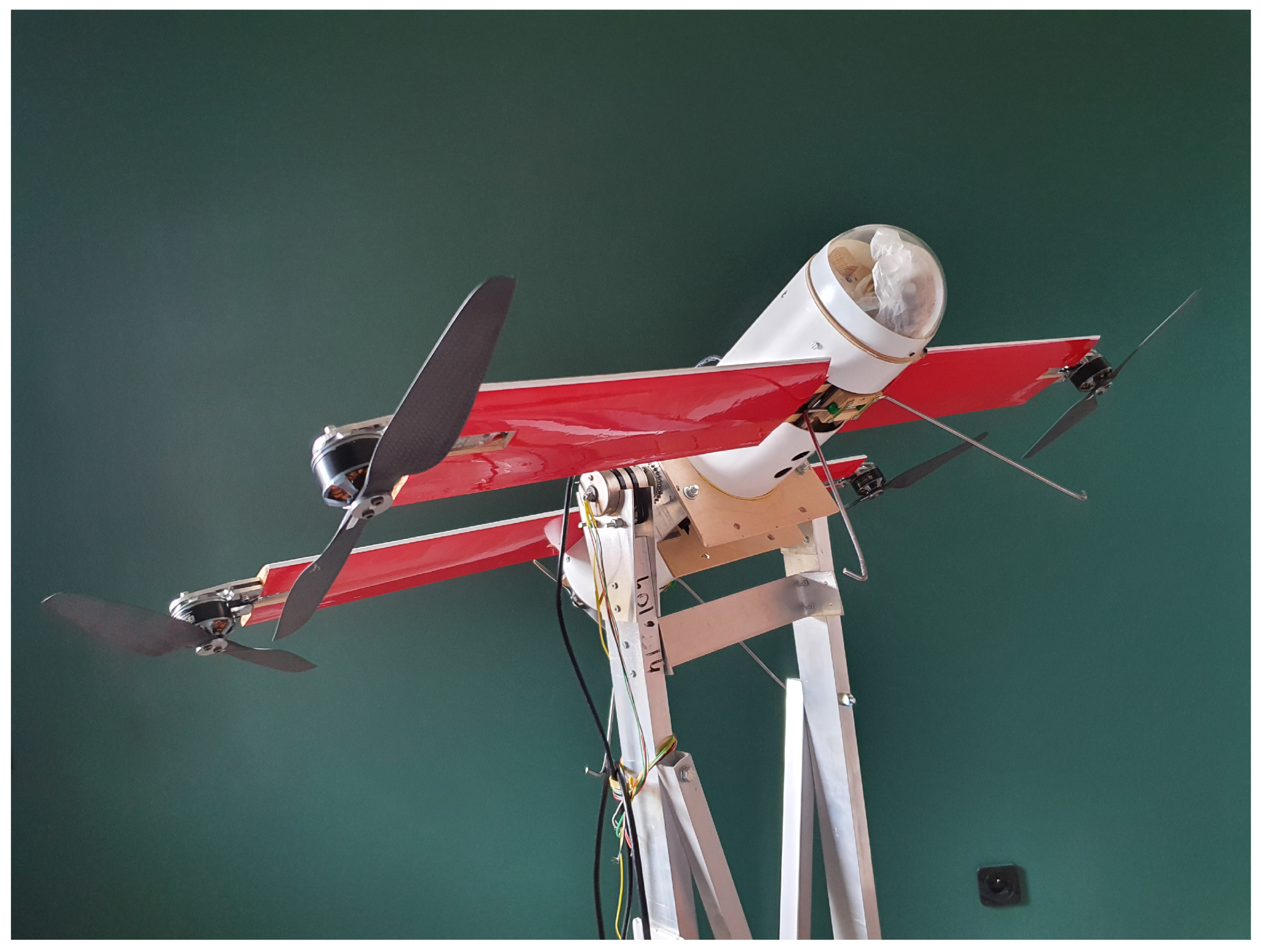
2.1. The Elka1Q Drone

We designed and built the Elka1Q drone shown in Figure 1. Besides some additional features, such as wings, it can fly like a regular quadcopter. The four main propulsion systems are optimized for long hovering and lifting a heavy payload: we mounted 4× T-Motor MN3110 KV470 with 12 × 4 carbon-fiber propellers. The main power source is a Li-Ion battery (6S3P). The drone’s flight controller uses an STM32F7 microcontroller running at 216 MHz. More technical details of the drone are described in [14,27]. The total weight of the drone depends on the selected sensor set but typically is ca. 3200 g.

2.2. On-Board Sensors’ Issues

The onboard IMU provides tilt angle measurements with great precision and accuracy—this has been tested prior to this research [28]. The IMU resolution, however, is an issue. The tilt angle measurements are read up to a centidegree (0.01°). According to the physical model of a quadcopter, [17,25], the angular speed (first derivative of the tilt angle) measurements are crucial to predict the drone state in subsequent time steps correctly.
We experimentally tested many smoothing techniques: low-pass filters, moving average filter, moving median filter, and many more. The key here is to balance the smoothing capabilities of the chosen filter and introduce as little signal delay as possible. Computational efficiency is essential as well—the filter is calculated ca. 20,000 times per second. The final filtering algorithm is described in the Appendix A.1. Figure 2 shows the filtering results. The filtered signal is smooth, and the introduced signal delay is acceptable (i.e., the attitude controller is stable in the whole range of tilt angle during the experiments with the drone’s hardware).

2.3. The Attitude Controller

The complete quadcopter’s dynamic equations are presented in [25], as well as the entire control stack. The attitude controller is just one of the controllers required by a quadcopter for flying. However, we claim it is the most important one. Any flight is impossible without that controller, including autonomous and fully manual flight scenarios. This is because of the unstable nature of such a flying vehicle. Many research works focus on an efficient trajectory planning or a high-level controller, assuming the attitude controller ‘as is’. We insist that a poor attitude controller can slow down or even lead to missing the desired trajectory while performing an autonomous flight. As described in [14,27], the quadcopter’s attitude control task can be decomposed into three parallel controllers. Indeed, the most common implementation consists of three independent PID (or even just PD) controllers, one for each axis: roll, pitch, and yaw. The roll and pitch controllers are usually the same type, sometimes having just slightly different values of the tuning parameters. Yaw control, however, is usually much slower and is not critical because a multicopter can actually fly in any direction, regardless of heading control. Usually, a slower PID or a Proportional (P) controller is good enough for the yaw axis stabilization. To simplify further considerations, we consider the pitch controller only in this paper.

2.4. A Novel Improvement for the Generalized Predictive Controller (GPC)

The GPC is an implementation of the MPC concept [11,12]. The key features of the GPC can be summarized as follows:
  • It relies on a linear model of a plant;
  • It works in a closed-loop (feedback);
  • It computes an optimal control signal for the whole control horizon (fixed number of discrete time steps), but only the very first control signal value is applied, and the others are discarded; in the next iteration of the control loop, the optimal control values are computed again (against the latest measurements);
  • The GPC is robust: even if the linear model does not match the real plant well, it can still control the system efficiently.
The control law of the classic (analytical) GPC is formulated:
Δ U ( k ) = K Y t ( k + 1 ) Y 0 ( k + 1 ) ,
where Δ U ( k ) is a vector of predicted control signal updates, K is the (fixed) control matrix which depends on the linear model of the object, and it is calculated off-line (only once). The  Y t ( k ) is the target (desired) trajectory at the moment k, and the Y 0 ( k ) is the free trajectory which depends on the linear model of the object and the past values of the real object: measurements and applied (past) control signal values. The linear model used in our experiments is described in the Appendix A.2. Sizes of matrices in Equation (1) depend on the fixed properties of the GPC: the prediction horizon N and the control horizon  N u :
Δ U ( k ) = Δ u ( k | k ) Δ u ( k + 1 | k ) Δ u ( k + N u | k ) N u × 1 = = K N u × N y t ( k + 1 | k ) y t ( k + 2 | k ) y t ( k + N + 1 | k ) N × 1 y 0 ( k + 1 | k ) + d ( k ) y 0 ( k + 2 | k ) + d ( k ) y 0 ( k + N + 1 | k ) + d ( k ) N × 1 ,
where d ( k ) is the modeling error: a difference between the latest measurement and the model prediction computed in the previous iteration:
d ( k ) = y ( k ) y ^ ( k | k 1 ) .
Typically, the future target trajectory Y t is unknown; thus, the values are constant:
Y t ( k + 1 ) = y t ( k + 1 | k ) y t ( k + 1 | k ) y t ( k + 1 | k ) N × 1 .
This approach works well for a GPC designed to keep the object at a fixed setpoint for a long time. The drones, however, continuously adjust the target attitude to maintain the hover position or to follow the flight trajectory. The drone dynamics restrict the range of feasible flight trajectories—if one is too aggressive, it will be simply physically impossible for a drone to follow it.
Known past values of the target attitude trajectory (and therefore its changes) and the intuition described above inspired us to propose a modification to the classic GPC: the Trajectory Guessing Algorithm.

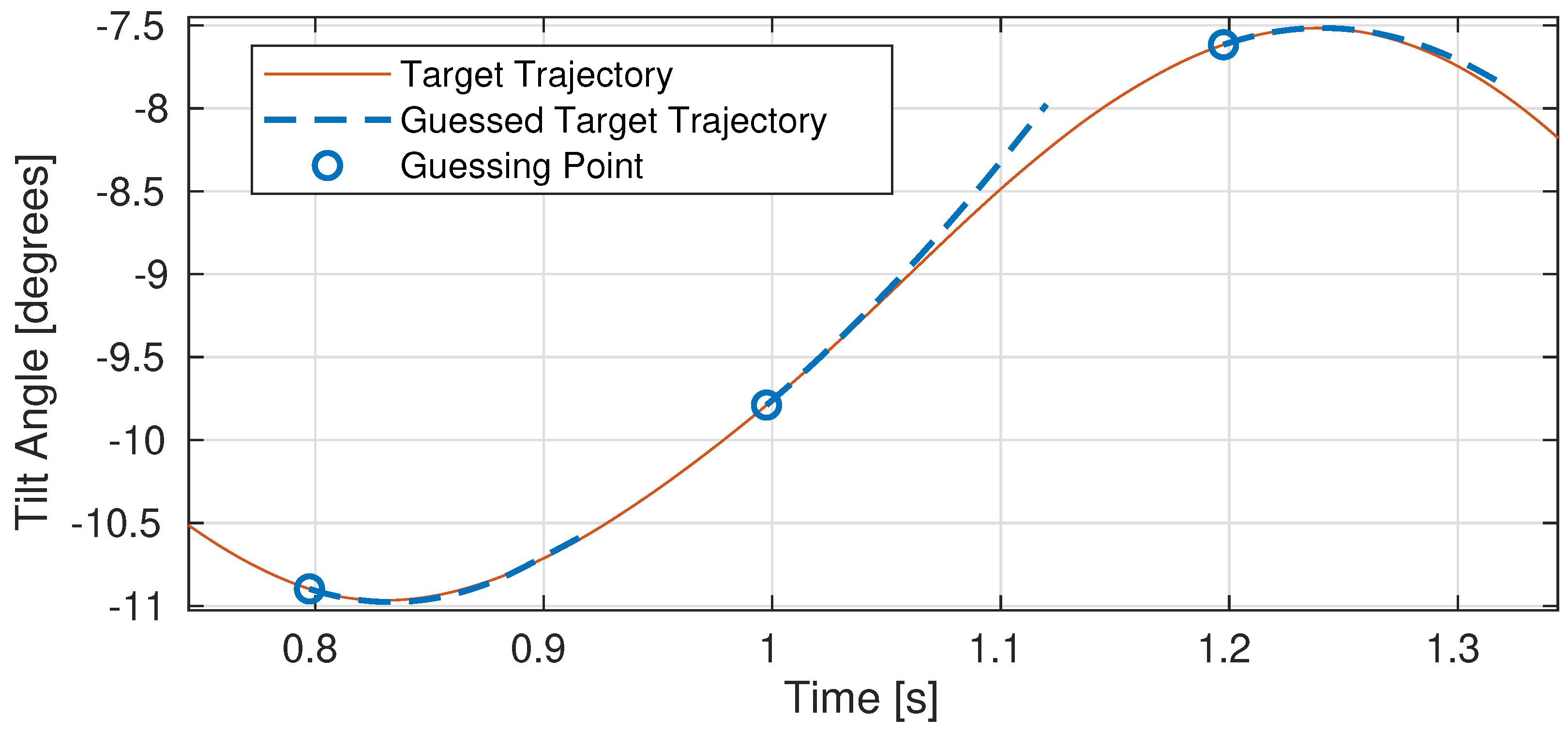
2.5. The Trajectory Guessing Algorithm

The target trajectory is a discrete signal. Let us define more differentiation equations (similarly to the Equation (A1)):
y ¨ t ( k ) = y ˙ t ( k ) y ˙ t ( k 1 ) , y ˙ t ( k ) = y t ( k ) y t ( k 1 ) = y ˙ t ( k 1 ) + y ¨ t ( k ) ,
where y t ( k ) is the target trajectory value at the moment k. We define the bound (cut-off) function as follows:
b ( x , x min , x max ) = { x max , if x x max , x min , if x x min , x , otherwise ,
and the bounds:
{ l 1 , l 2 } = { { y ˙ t ( k ) , β y ˙ t ( k ) } ,        if sgn ( y ˙ t ( k ) ) = sgn ( y ¨ t ( k ) ) , { β y ˙ t ( k ) , y ˙ t ( k ) } ,   otherwise , y ˙ t m i n = min { l 1 , l 2 } , y ˙ t m a x = max { l 1 , l 2 } ,
where the β = 1.5 was found experimentally. The final bound function formula looks as follows:
b y ( y t ) = b ( y t , y ˙ t m i n , y ˙ t m a x ) .
The following recurrent equations describe the Trajectory Guessing Algorithm:
y ˙ ^ t ( k + 1 | k ) = b y y ˙ t ( k | k ) + y ¨ t ( k ) , y ˙ ^ t ( k + 2 | k ) = b y y ˙ ^ t ( k + 1 | k ) + y ¨ t ( k ) , y ˙ ^ t ( k + N | k ) = b y y ˙ ^ t ( k + N 1 | k ) + y ¨ t ( k ) ,
and, consequently,
y t ( k + 1 | k ) = y t ( k | k ) + y ˙ ^ t ( k | k ) , y t ( k + 2 | k ) = y t ( k + 1 | k ) + y ˙ ^ t ( k + 1 | k ) , y t ( k + N | k ) = y t ( k + N 1 | k ) + y ˙ ^ t ( k + N | k ) .
Please note that the predicted second derivative of the target trajectory is constant:
y ¨ t ( k + 1 | k ) = y ¨ t ( k + 2 | k ) = = y ¨ t ( k + N | k ) = y ¨ t ( k ) .
The above Equations (5)–(11) explain how the prediction of the future target trajectory relies on the past discrete derivative values (namely, first and second derivative). The method has two main assumptions: the second derivative remains constant over the prediction horizon (in our case: 30 steps); the changing (predicted) first derivative values are limited to some bounds, calculated for the most recent target trajectory values.
The Trajectory Guessing Algorithm results are presented in Figure 3, where an artificial target trajectory is used to visualize the concept better.

2.6. Assessment Methods
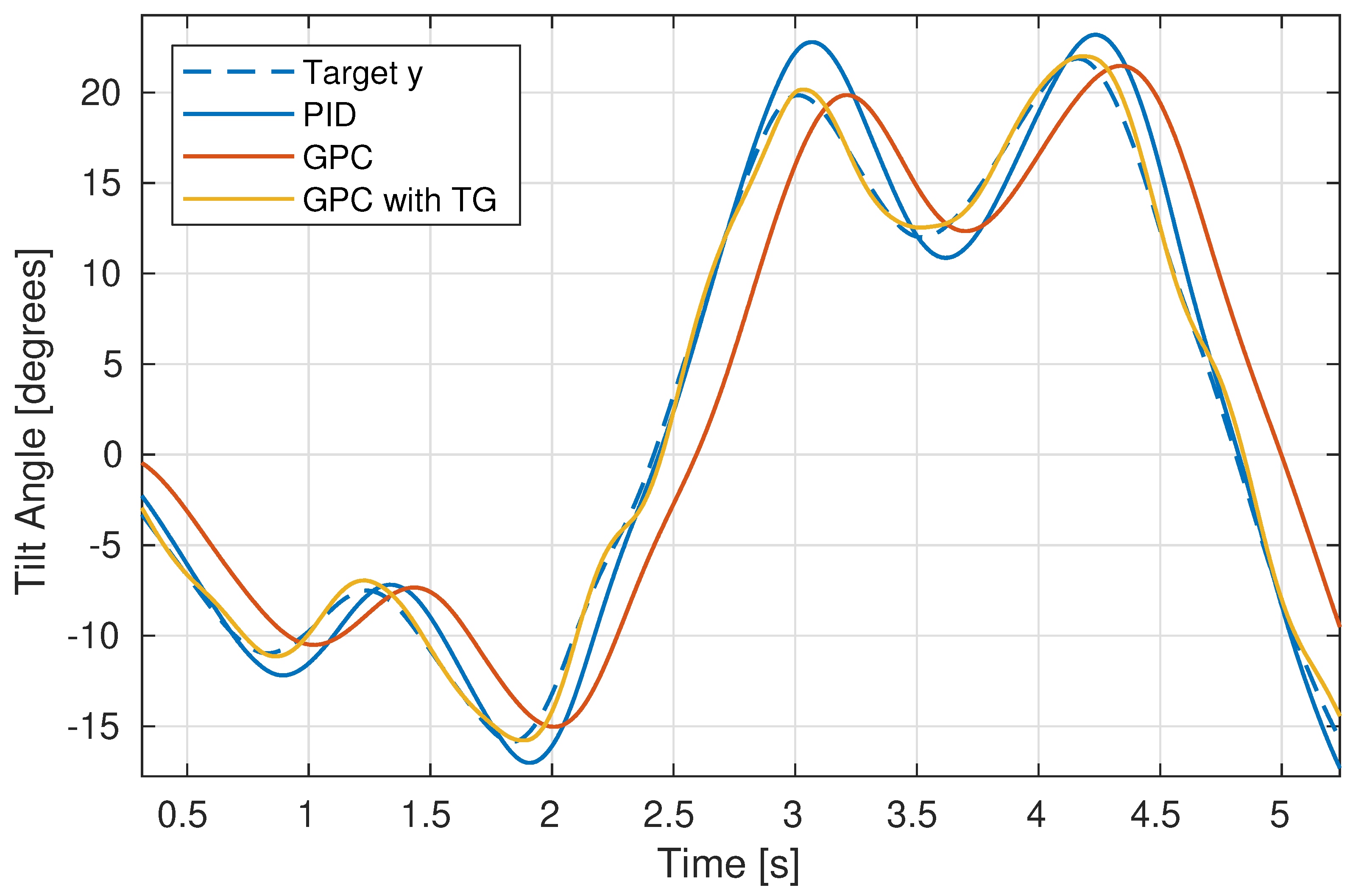
It is important to compare subsequent attitude controller implementations in the same, well-controlled conditions. To address that need, we implemented a custom Flight Mode [29] for the ArduCopter software: the Fixed Trajectory Mode. We took a 30-second-long part of telemetry data from one of the real flight experiments. The extracted target pitch angle trajectory has been hardcoded into the new Fixed Trajectory Mode, overriding any incoming target pitch angle signals. We turned off the roll and the yaw attitude controllers because the drone was locked in a well-balanced harness that allows tilting the drone over a single axis only (pitch). We designed the harness in such a way that the drone rotates exactly over its center of mass—as in an actual hover flight (see Figure 1). Additionally, the harness is tall enough to minimize undesired air gusts caused by the airflow (from the main propellers) bounced back by the floor.
The idea behind the Trajectory Guessing Algorithm was simple: make the attitude controller as quick and as accurate as possible. Therefore, we used Matlab’s finddelay [30] function as the metric of the overall delay of the controller.
We used the drone’s onboard current and voltage sensors to measure the total energy consumption. The sensors were able to produce ca. 200 readings per second.
The controller’s delay and the total electric power consumption are compared below while discussing the final results of a series of experiments based on the Fixed Trajectory Mode.

3. Results

The Fixed Trajectory Mode (described in Section 2.6) was necessary to perform a repetitive, precise comparison of all the attitude controllers mentioned in this paper: PID, the original MPC, and the MPC with novel modification: the Trajectory Guessing Algorithm. The overall results are shown in Figure 4. More details of controllers’ delay and accuracy can be observed in a zoomed part of the experiment in Figure 5. The total energy consumption of all the controllers (during the Fixed Trajectory experiment) is shown in Figure 6. The total energy consumption difference, where PID Controller is taken as the baseline, is presented in Figure 7. The total peak power usage is shown in Figure 8 and Figure 9. Please note that the average power needed for the drone to hover is about 270 W, but it can use even up to three times higher peak power (ca. 1 kW) to aggressively tilt the drone to the desired position.
We summarized the final results (a median from five experiment runs) in Table 1.

4. Discussion

Modern flying UAVs have to be more agile as they operate in more demanding environments, e.g., urban or post-disaster areas. For example, speed and agility are critical for robust obstacle avoidance in medical supply or SAR missions. Without using extra-long range sensors, the only way to let them fly faster (but still safely) is to increase the maneuverability. We were sure it was still possible to achieve that without extra hardware modifications. Therefore, we focused on finding possible flight controller improvements and estimating the total energetic cost of such agility.
First, we selected a simple assessment metric to compare the software improvements: the delay introduced by an attitude controller. Then, we had to be sure that the subsequent experiments were comparable. We implemented a new Flight Mode in the ArduCopter software to repeat a fixed (hardcoded) trajectory. Then we mounted the drone in a harness, which locks all its degrees of freedom but pitch.
Prior to this research, we ensured the PID was well tuned (manually and via the Auto-Tune Mode). We studied the telemetry data and found that the PID controller works fine but is not as fast and accurate as we thought it should be in a genuinely agile drone. The MPC was the next natural choice to test. We implemented the GPC variant, based on a linear Neural Network model found in our previous research [14]. The results, however, were not satisfying. Although the MPC was accurate, it was even slower than the original PID—it can be observed in Figure 5. Tuning the MPC’s horizons and delta parameter leads to unstable controller behavior, most likely due to modeling errors.
Based on the observed phenomena, we proposed a novel modification to the original MPC: the Trajectory Guessing Algorithm. This modification was simple enough to be implemented in the high-frequency onboard attitude controller (running at 400 Hz, keeping in mind the limited resources of the drone’s flight controller hardware). Achieved speed-up of the stable MPC was impressive; however, as expected, the outstanding agility comes with a higher total energy consumption: about 15.7% more than the default PID. The results are presented in Figure 5 and in Table 1.
We have an idea of how to maximize the benefits of the implemented Attitude Controller, despite its higher power consumption. The drone could have a hybrid (or multi-level) attitude controller: a slow one, e.g., the default PID, when it flies through an environment where not many obstacles are expected (high-altitude flights), and it could switch to the agile controller when it approaches a more demanding environment such as flying through an urban area at low altitude.
One may argue that the energetic cost for the achieved agility is too high, and similar results, i.e., increasing the average flight speed, could be solved simply by installing better range sensors for improved obstacle avoidance. Better range sensors could give the drone more time for more efficient path planning so that the drone could start a sufficient maneuver sooner. However, having such (better) sensors implies that the drone could fly even faster if it just has better maneuverability, thus having a rapid attitude controller, which brings us again to the fundamental concept of this research.
The above considerations suggest an interesting idea for future research: to check how much faster a drone could fly through a fixed, non-trivial path with a more agile attitude controller. It could be either simulated or a real flight experiment. The answer is not easy to predict: a sharper attitude controller consumes more energy but allows the drone to fly faster, which reduces the total flight time to the target destination. Will the shorter (but faster) flight consume less or actually more energy?
Another future research topic may focus on finding a different way to improve the drone’s maneuverability with lower energetic cost, which could be through software, hardware, or aerodynamic modification. An exciting example of such a modification is described in [25] (a combination of hardware and control system modifications), but the energetic cost is not discussed there.

5. Conclusions

The drones market is increasing rapidly. This has inspired researchers to develop better drones: ones that are smarter and fly longer, faster, and farther away. Critically, agile drones are necessary for many scenarios, including but not limited to medical supply and SAR missions. We state that a drone can fly faster and with greater agility if it has a more aggressive attitude controller onboard. We focused on improving the attitude controller algorithm and assumed no other hardware modifications of the drone. Ultimately, we proposed a novel modification to the MPC controller: the Trajectory Guessing Algorithm, which drastically improved the drone’s maneuverability. We assessed the new attitude controller against the most common implementation (PID) in a custom-implemented Flight Mode (Fixed Trajectory Mode) in the ArduCopter software stack. We found that our modified MPC is much faster than PID. The total increase in power demand is higher by 15.7% over PID.

Author Contributions

Conceptualization, M.O. and M.Ł.; methodology, M.O. and M.Ł.; software, M.O.; validation, M.O.; formal analysis, M.O. and M.Ł.; investigation, M.O.; resources, M.O.; data curation, M.O.; writing—original draft preparation, M.O.; writing—review and editing, M.O. and M.Ł.; visualization, M.O.; supervision, M.Ł.; project administration, M.Ł. All authors have read and agreed to the published version of the manuscript.

Funding

This research received no external funding.

Institutional Review Board Statement

Not applicable.

Informed Consent Statement

Not applicable.

Data Availability Statement

Not applicable.

Conflicts of Interest

The authors declare no conflict of interest.

Abbreviations

The following abbreviations are used in this manuscript:
UAVUnmanned Aerial Vehicle
SARSearch-and-Rescue
PIDProportional-Integral-Derivative
PDProportional-Derivative
IMUInertial Measurement Unit
MPCModel Predictive Controller
GPCGeneralized Predictive Controller

Appendix A

Appendix A.1. The Trajectory Smoothing Algorithm

The tilt angle is a discrete signal. Let us define the following differentiation equations:
y ˙ ( k ) = y ( k ) y ( k 1 )
The final formula of the implemented filter looks as follows:
s = ( n 1 ) 1.1 + 0.9 , y 1 = y f ( k n ) y f ( k n + 1 ) y f ( k 2 ) y f ( k 1 ) , y 2 = y 1 y ( k ) ,
and according to the differentiation Equation (A1):
y ˙ 2 = y f ( k n + 1 ) y f ( k n ) y f ( k 1 ) y f ( k 2 ) y ( k ) y f ( k 1 ) , y f ( k ) = y f ( k 1 ) + 1 s i = 1 n 1 1.1 y ˙ 2 ( i ) + 0.9 y ˙ 2 ( n ) ,
where n = 7 , y f ( k ) is the filtered (smoothed) tilt angle value, y ( k ) is the latest (measured) tilt angle value (noised), y 2 is a helper vector containing smoothed tilt angle values (except the last one), and y ˙ 2 is a helper vector with angular speed values (the first derivative of the discrete signal y 2 using the Equation (A1)).
The fundamental concept of the proposed algorithm is to predict the smoothed difference value (the first derivative) of the latest signal sample. The prediction is made on the weighted first derivative values of a few past (smoothed) samples and the single, most recent, unfiltered (raw) sample. The algorithm comprises a good smoothing performance with the introduction of a minimal signal delay.
See Figure 2 for the filtering results.

Appendix A.2. The Neural-Network-Based Linear Model

We identified and tested a wide variety of linear and non-linear models [14,27]. Next, we selected the most promising subset to be implemented onboard. After a series of experiments, we rejected the most complex ones and focused on a few fastest and most reliable neural-based linear models. Further experiments proved that the simple One-Step-Forward neural linear model works well as a base model for the GPC. We found the tuning parameters of the model structure experimentally. The final model structure looks as follows:
y 0 ( k + 1 | k ) = w · x ( k ) ,
where w is the neuron’s weight vector:
w = w 1 w 2 w 7 ,
and x is the vector of input values:
x ( k ) = y ˙ ( k ) y ¨ ( k ) u ( k 1 ) u ( k 2 ) u ( k 5 ) ,
where we have the first and second derivative of the tilt angle, see Equation (5), and later on the last five control signal values.
Further predictions of the model are computed recurrently: a given predicted value is used to calculate the tilt angle derivatives, and then to calculate the next model output:
y ˙ ( k ) = y ( k ) y ( k 1 ) , y ˙ ( k 1 ) = y ( k 1 ) y ( k 2 ) , y ¨ ( k ) = y ˙ ( k ) y ˙ ( k 1 ) , y 0 ( k + 1 | k ) = w · [ y ˙ ( k )   y ¨ ( k )   u ( k 1 )     u ( k 5 ) ] ,
y ˙ ( k + 1 ) = y 0 ( k + 1 | k ) y ( k ) , y ˙ ( k ) = y ( k ) y ( k 1 ) , y ¨ ( k + 1 ) = y ˙ ( k + 1 ) y ˙ ( k ) , y 0 ( k + 2 | k ) = w · [ y ˙ ( k + 1 )   y ¨ ( k + 1 )   u ( k 1 )   u ( k 1 )     u ( k 4 ) ] ,
y ˙ ( k + 2 ) = y 0 ( k + 2 | k ) y 0 ( k + 1 | k ) , y ˙ ( k + 1 ) = y 0 ( k + 1 | k ) y ( k ) , y ¨ ( k + 2 ) = y ˙ ( k + 2 ) y ˙ ( k + 1 ) , y 0 ( k + 3 | k ) = w · [ y ˙ ( k + 2 )   y ¨ ( k + 2 )   u ( k 1 )   u ( k 1 )   u ( k 1 )     u ( k 3 ) ] ,
and so on. Please note the future control signals u ( k ) , u ( k + 1 ) , etc., are unknown; therefore, only past control signals are used: from the oldest: u ( k 5 ) up to the latest known value: u ( k 1 ) .
There is at least one important benefit of representing such a simple linear model as a neural network (in fact: as a single linear neuron, with no bias input). We can use modern GPU-optimized libraries, such as Tensorflow 2 [31] and Keras [32] for training the neuron, i.e., for finding the weight vector.

References

  1. Máthé, K.; Buşoniu, L. Vision and control for UAVs: A survey of general methods and of inexpensive platforms for infrastructure inspection. Sensors 2015, 15, 14887–14916. [Google Scholar] [CrossRef] [PubMed] [Green Version]
  2. Waharte, S.; Trigoni, N. Supporting search and rescue operations with UAVs. In Proceedings of the 2010 International Conference on Emerging Security Technologies, Canterbury, UK, 6–7 September 2010; pp. 142–147. [Google Scholar]
  3. Aljehani, M.; Inoue, M. Performance Evaluation of Multi-UAV System in Post-Disaster Application: Validated by HITL Simulator. IEEE Access 2019, 7, 64386–64400. [Google Scholar] [CrossRef]
  4. Heutger, M.; Kückelhaus, M. Unmanned Aerial Vehicles in Logistics a DHL Perspective on Implications and Use Cases for the Logistics Industry; DHL Customer Solutions & Innovation: Troisdorf, Germany, 2014. [Google Scholar]
  5. Razi, P.; Sumantyo, J.T.S.; Perissin, D.; Kuze, H.; Chua, M.Y.; Panggabean, G.F. 3D Land Mapping and Land Deformation Monitoring Using Persistent Scatterer Interferometry (PSI) ALOS PALSAR: Validated by Geodetic GPS and UAV. IEEE Access 2018, 6, 12395–12404. [Google Scholar] [CrossRef]
  6. Scott, J.E.; Scott, C.H. Drone Delivery Models for Medical Emergencies. In Delivering Superior Health and Wellness Management with IoT and Analytics; Springer: Cham, Switzerland, 2020; pp. 69–85. [Google Scholar]
  7. Alicandro, M.; Dominici, D.; Massimini, V. Surveys with UAV photogrammetry: Case studies in l’Aquila during the post-earthquake scenario. In Proceedings of the EGU General Assembly Conference Abstracts, Vienna, Austria, 12–17 April 2015; p. 14987. [Google Scholar]
  8. Perez-Grau, F.; Ragel, R.; Caballero, F.; Viguria, A.; Ollero, A. Semi-autonomous teleoperation of UAVs in search and rescue scenarios. In Proceedings of the 2017 International Conference on Unmanned Aircraft Systems (ICUAS), Miami, FL, USA, 13–16 June 2017; pp. 1066–1074. [Google Scholar] [CrossRef]
  9. Euchi, J. Do drones have a realistic place in a pandemic fight for delivering medical supplies in healthcare systems problems? Chin. J. Aeronaut. 2021, 34, 182–190. [Google Scholar] [CrossRef]
  10. Maheswari, R.; Ganesan, R.; Venusamy, K. MeDrone- A Smart Drone to Distribute Drugs to Avoid Human Intervention and Social Distancing to Defeat COVID-19 Pandemic for Indian Hospital. J. Phys. Conf. Ser. 2021, 1964, 062112. [Google Scholar] [CrossRef]
  11. Camacho, E.F.; Bordons, C. Model Predictive Control; Springer: London, UK, 1999. [Google Scholar]
  12. Tatjewski, P. Advanced Control of Industrial Processes: Structures and Algorithms; Springer Science & Business Media: London, UK, 2007. [Google Scholar]
  13. Åström, K.J.; Murray, R.M. Feedback Systems; Princeton University Press: Princeton, NJ, USA, 2010. [Google Scholar]
  14. Okulski, M.; Ławryńczuk, M. A Novel Neural Network Model Applied to Modeling of a Tandem-Wing Quadplane Drone. IEEE Access 2021, 9, 14159–14178. [Google Scholar] [CrossRef]
  15. Valavanis, K.P.; Vachtsevanos, G.J. Handbook of Unmanned Aerial Vehicles; Springer: Dordrecht, The Netherlands, 2015; Volume 1. [Google Scholar]
  16. Yang, H.; Lee, Y.; Jeon, S.Y.; Lee, D. Multi-rotor drone tutorial: Systems, mechanics, control and state estimation. Intell. Serv. Robot. 2017, 10, 79–93. [Google Scholar] [CrossRef]
  17. Mahony, R.; Kumar, V.; Corke, P. Multirotor aerial vehicles: Modeling, estimation, and control of quadrotor. IEEE Robot. Autom. Mag. 2012, 19, 20–32. [Google Scholar] [CrossRef]
  18. Andropov, S.; Guirik, A.; Budko, M.; Budko, M.; Bobtsov, A. Synthesis of Artificial Network Based Flight Controller Using Genetic Algorithms. In Proceedings of the 2018 10th International Congress on Ultra Modern Telecommunications and Control Systems and Workshops (ICUMT), Moscow, Russia, 5–9 November 2018; pp. 1–5. [Google Scholar]
  19. Muñoz, F.; González-Hernández, I.; Salazar, S.; Espinoza, E.S.; Lozano, R. Second order sliding mode controllers for altitude control of a quadrotor UAS: Real-time implementation in outdoor environments. Neurocomputing 2017, 233, 61–71. [Google Scholar] [CrossRef]
  20. Koch, W.; Mancuso, R.; West, R.; Bestavros, A. Reinforcement learning for UAV attitude control. ACM Trans. Cyber-Phys. Syst. 2019, 3, 1–21. [Google Scholar] [CrossRef] [Green Version]
  21. Shin, J.; Kim, H.J.; Park, S.; Kim, Y. Model predictive flight control using adaptive support vector regression. Neurocomputing 2010, 73, 1031–1037. [Google Scholar] [CrossRef]
  22. Misin, M.; Puig, V. LPV MPC Control of an Autonomous Aerial Vehicle. In Proceedings of the 2020 28th Mediterranean Conference on Control and Automation (MED), Saint-Raphael, France, 15–18 September 2020; pp. 109–114. [Google Scholar] [CrossRef]
  23. Grujic, I.; Nilsson, R. Model-based development and evaluation of control for complex multi-domain systems: Attitude control for a quadrotor uav. Tech. Rep. Electron. Comput. Eng. 2016, 4. [Google Scholar]
  24. Shauqee, M.N.; Rajendran, P.; Suhadis, N.M. Quadrotor Controller Design Techniques and Applications Review. INCAS Bull. 2021, 13, 179–194. [Google Scholar] [CrossRef]
  25. Tal, E.; Karaman, S. Accurate Tracking of Aggressive Quadrotor Trajectories Using Incremental Nonlinear Dynamic Inversion and Differential Flatness. IEEE Trans. Control Syst. Technol. 2021, 29, 1203–1218. [Google Scholar] [CrossRef]
  26. Ryou, G.; Tal, E.; Karaman, S. Multi-fidelity black-box optimization for time-optimal quadrotor maneuvers. arXiv 2020, arXiv:2006.02513. [Google Scholar]
  27. Okulski, M.; Ławryńczuk, M. Identification of Linear Models of a Tandem-Wing Quadplane Drone: Preliminary Results. In Advanced, Contemporary Control; Springer: Cham, Switzerland, 2020; pp. 219–228. [Google Scholar]
  28. Okulski, M.; Ławryńczuk, M. Development of a High-Efficiency Pitch/Roll Inertial Measurement Unit Based on a Low-Cost Accelerometer and Gyroscope Sensors. In Proceedings of the 2019 24th International Conference on Methods and Models in Automation and Robotics (MMAR), Międzyzdroje, Poland, 26–29 August 2019; pp. 657–662. [Google Scholar]
  29. Adding a New Flight Mode to Copter. 2021. Available online: https://ardupilot.org/dev/docs/apmcopter-adding-a-new-flight-mode.html (accessed on 11 November 2021).
  30. Matlab’s Finddelay Function Reference. 2021. Available online: https://www.mathworks.com/help/signal/ref/finddelay.html (accessed on 11 November 2021).
  31. API Documentation | TensorFlow Core r2.1. 2021. Available online: https://www.tensorflow.org/api_docs/ (accessed on 1 November 2021).
  32. Keras: The Python Deep Learning Library. 2021. Available online: https://keras.io/ (accessed on 11 November 2021).
Figure 1. The Elka1Q drone.
Energies 15 01380 g001
Figure 2. The raw tilt angle signal (from the IMU) and the results of the Smoothing Algorithm.
Energies 15 01380 g002
Figure 3. An example of results of the Trajectory Guessing Algorithm.
Energies 15 01380 g003
Figure 4. The Fixed Trajectory Experiment: complete target trajectory and the highlighted part of the experiment.
Energies 15 01380 g004
Figure 5. Performance of all the controllers for a selected part of the Fixed Trajectory Experiment.
Energies 15 01380 g005
Figure 6. Total energy consumption during the Fixed Trajectory Experiment for all the controllers.
Energies 15 01380 g006
Figure 7. Total energy consumption during the Fixed Trajectory Experiment: MPC compared to PID.
Energies 15 01380 g007
Figure 8. Power usage during the selected part of the Fixed Trajectory Experiment: MPC (with Trajectory Guessing) compared to PID.
Energies 15 01380 g008
Figure 9. The peak power usage histogram during the Fixed Trajectory Experiment: MPC (with Trajectory Guessing) compared to PID.
Energies 15 01380 g009
Table 1. Comparison of the attitude controllers.
ControllerDelayEnergy Consumption
PID243.50 Wh
MPC743.35 Wh
MPC with Trajectory Guessing64.05 Wh
Publisher’s Note: MDPI stays neutral with regard to jurisdictional claims in published maps and institutional affiliations.

