Long-Horizon Nonlinear Model Predictive Control of Modular Multilevel Converters

Abstract

Modular Multilevel Converters (MMCs) are a topology that can scale several voltage levels to obtain higher efficiency and lower harmonics than most voltage-source converters. MMCs are very attractive for renewable energy applications and fast charging stations for electric vehicles, where they can improve performance and reduce costs. However, due to the complex architecture and the large number of submodules, the current control of modular multilevel converters is a challenging task. The standard solution in practice relies on hierarchical decoupling and single-input-single-output control loops, which are limited in performance. Linearization-based model predictive control was already proposed for current control in MMCs, as it can optimize transient response and better handle constraints. In this paper, we show that the validity of linear MMC models significantly limits the prediction horizon length, and we propose a nonlinear MPC (NMPC) solution for current control in MMCs to solve this issue. With NMPC, we can employ long prediction horizons up to 100 compared to a horizon of 10, which is the limit for the prediction range of a linear MMC model. Additionally, we propose an alternative MMC prediction model and corresponding cost function, which enables directly controlling the circulating current and improves the capacitor voltages’ behavior. Using the state-of-the-art in sequential quadratic programming for NMPC, we show that the developed NMPC algorithm can meet the real-time constraints of MMCs. A performance comparison with a time-varying linearization-based MPC for an MMC topology used in ultra-fast charging stations for electric vehicles illustrates the benefits of the developed approach.

1. Introduction

The Modular Multilevel Converters (MMCs) topology was presented in [1]. This type of power electronics hardware has as its main feature a series connection of module capacitors called submodules (see Figure 1). Employing these submodules allows scaling a higher number of output voltage levels. Performance-wise, this characteristic permits obtaining a low-current total harmonic distortion (THD) regardless of the switching frequencies [2]. Other advantages of MMCs include transformerless operational capability and increased fault-tolerance [3]. Compared to other existing voltage-source converters (VSCs), MMCs are considered more efficient and reliable solutions for high- and medium-power applications; see e.g., [4,5]. These applications include ultra-fast charging stations (UFCSs) of electric vehicles (EVs); see e.g., [6,7]. In this novel application, the MMC should ensure bidirectional power transfer between the grid and the DC bus with lower losses and perturbation to the grid.

MMCs have a modular design in which their submodules are interconnected physically. These submodules have nonlinear and discontinuous dynamics due to switching, and the proper functioning of the MMCs depends on the coordinated actions of these submodules. Hence, MMCs are multiple-inputs-multiple-outputs (MIMO) complex systems [8]. Regardless of the application, the control objectives of the MMCs are (i) tracking of a time-varying reference for the output currents, (ii) maintaining the average capacitor voltages around a nominal value, (iii) suppressing the circulating current and (iv) balancing the capacitor voltages. However, these control objectives cannot be achieved simultaneously, which further adds to the challenge of controller design for MMCs.

Hierarchical PI (proportional–integral) single-input-single-output control schemes are well-established control solutions for these systems, see e.g., [9,10], but they are quite limited in performance. Model predictive control (MPC) has achieved promising results improving the transient response of MMCs, see e.g., [2,11,12,13], as it allows finding a Pareto optimal solution to the multiple control objectives relevant for MMCs and handles constraints. In general, the MPC solutions for MMCs are of two types: finite-control-set MPC [11,12,13,14], which directly controls the discrete valued switching signals, and standard, continuous-control-set MPC [2,15,16,17], which computes continuous insertion indexes and then utilizes modulation techniques to control the switches. While finite-control-set MPC holds a promise for the future, currently, its implementation is limited by the combinatorial increase in complexity with the increase of the prediction horizon and the number of submodules. In general, a long prediction horizon is desired when tracking time-varying references and for optimizing the efficiency of power electronics circuits, see, e.g., [18,19]. Hence, in this paper, we focus on continuous-control-set MPC (CCS-MPC), which in general exhibits a tractable complexity increase with the increase of the prediction horizon.

In [2], a successive linearization-based MPC solution for current control in MMCs with prediction horizon $N_p=6$ (this was extended to $N_p=10$ in [18]) showed improvement over alternative solutions such as finite-control-set MPC and hierarchical PI schemes. Therein, a cost for regulating the capacitor voltages behavior was also proposed. In [15,16], the bilinear relationship between the arm current and the capacitor voltage that describes the arm voltage dynamics is disregarded. Consequently, a linear model is obtained by defining the arm voltage as the control input of the system. However, the validity of such a linear model is limited to short prediction horizons ($N_p=1$ was used in these papers) since the dependency between the control input and the state is not considered. In [17], the authors built a model of the MMC in the dq-framework. This approach also yields a linear model of the system and shows good performance with a prediction horizon $N_p=4$. However, extending this solution to MMC systems working under unbalanced conditions is challenging.

All of the above CSS-MPC solutions based on linear or time-varying linear models obtained via online linearization can be implemented as a single quadratic programming (QP) problem, which can be solved efficiently. In principle, QP solvers for MPC allow using a much longer prediction horizon compared to finite-control-set MPC. However, as shown in this paper, the validity of linear MMC models is limiting the prediction horizon length for which accurate predictions can be obtained, because the current dynamics of MMCs are essentially bilinear dynamics with a strong nonlinear behavior. It is also worth mentioning that recently, a differential-flatness nonlinear control solution for MMCs was developed in [20] and a neural networks based nonlinear MPC controller with a short prediction horizon ($N_p=3$) for MMCs was proposed in [21].

Motivated by the above analysis and the advances in sequential quadratic programming (SQP) solvers for nonlinear MPC (NMPC) [22,23], in this paper, we develop a continuous-control-set long-horizon NMPC algorithm for current control in MMCs. The NMPC controller optimizes a cost function that penalizes the above-mentioned (i)–(iii) objectives subject to constraints. We derive a nonlinear MMC prediction model using a per-phase approach, which allows accurate predictions over a long, 200-steps horizon, compared to a 10-steps horizon corresponding to a linearized MMC model. Additionally, we construct the MMC prediction model differently than done in the previous linear MPC solutions, e.g., [2], to enable direct control of the circulating current and to improve the capacitor voltages behavior. The developed NMPC algorithm computes a voltage reference for a carrier-based PWM (CB-PWM) modulator, and the capacitor voltage balancing is performed separately using the method proposed in [9]. To compare the developed NMPC solution with an online linearization-based MPC solution, we consider a specific MMC topology designed for ultra-fast charging stations of electric vehicles, as in [7]. The obtained results show a reduction of 29% of the power losses and 98% efficiency when a long-horizon NMPC controller is used. Moreover, we present the computational time of running the NMPC using the ACADO toolkit interface with MATLAB. Based on those results and the capacity of field-programmable gate array (FPGA) to outperform microprocessor implementations in terms of computational speed [24], the developed NMPC algorithm can be implemented in real time for much longer prediction horizons (i.e., $N_p=25$ up to $N_p=100$ compared to previous MPC solutions for MMCs surveyed above that use $N_p=1$ up to $N_p=10$).

The remainder of the paper is structured as follows. Section 2 describes the MMC topology along with the derivation of linear and nonlinear prediction models. After that, the MMC control problem is formulated in Section 3. The design and implementation of the NMPC algorithm for MMCs is presented in Section 4. Realistic simulation results and comparison with linearization-based MPC for MMCs are presented in Section 5. Conclusions are summarized in Section 7.

Notation: Let $\mathbb{R}$, ${\mathbb{R}}_{+}$, $\mathbb{Z}$, and ${\mathbb{Z}}_{+}$ denote the field of real numbers, the set of non-negative reals, the set of integer numbers, and the set of non-negative integers, respectively. The quadratic norm of a vector $x\in {\mathbb{R}}^n$ weighted by a positive-definite matrix $Q=Q^{\top }\in {\mathbb{R}}^{n\times n}$ is denoted by ${\left|x\right|}_Q^2:=x^{\top }Qx$. The identity matrix is denoted by ${\mathbb{I}}_n\in {\mathbb{R}}^{nxn}$. For a set $\mathbb{S}\subseteq {\mathbb{R}}^n$, define ${\mathbb{S}}_{[a,b]}:=\{s\in \mathbb{S}:a\le s\le b\}$ and ${\mathbb{S}}^N:=\mathbb{S}\times \dots \times \mathbb{S}$.

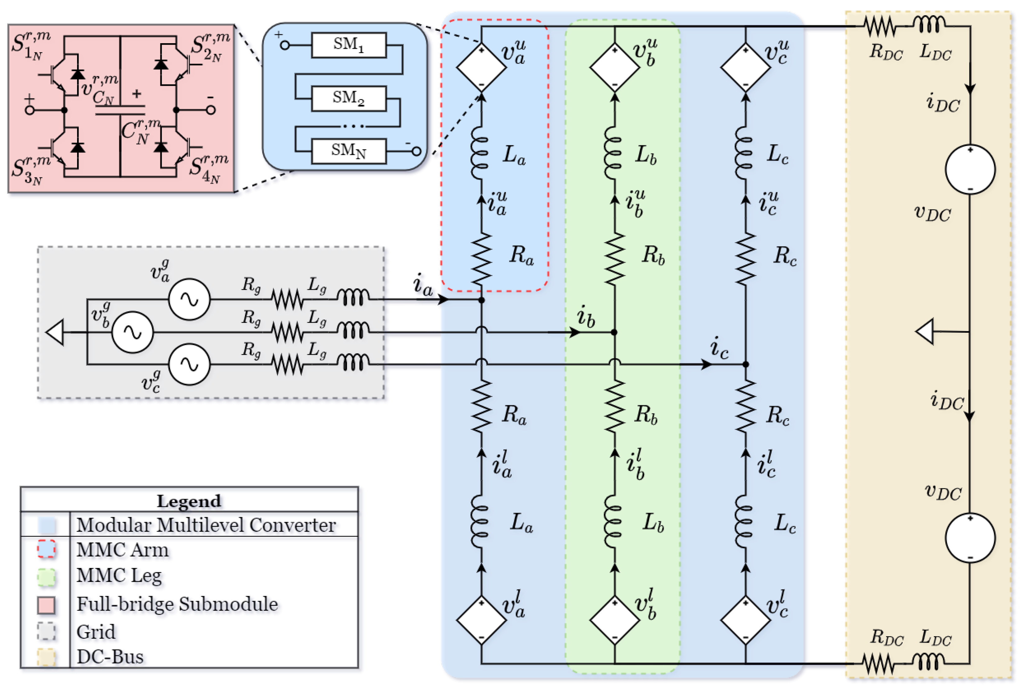
2. Modular Multilevel Converter Topology and Modeling

This section presents a general description of an MMC topology meant for usage in a ultra-fast charging station (UFCS) for electric vehicles instead of a traditional transformer solution [25,26]. A description of the MMC topology is given, and the differential equations describing the behavior of the internal variables of the MMC are derived.

2.1. MMC Topology for Utra-Fast Charging Stations

The studied MMC is configured using the topology presented in [7]; see Figure 1. The MMC is generally comprising of three-phase legs $m\in \{a,b,c\}$, each with two arms $r\in \{u,l\}$. The arms are composed of N submodules (SM) connected in series, an arm inductor $(L_m)$, and an arm resistance $(R_m)$ that models conduction and device losses of the arm.

The topology of the submodules is a full-bridge (FB), i.e., they are composed of a polarized capacitor $(C_N^{r,m}=C)$ and four IGBTs. The IGBTs are driven by gating signals that determine the switching signals $({\overline{S}}^{r,m})$ and the corresponding terminal voltage of the submodule $(v_{SM})$, as described in

Table 1. Relationship among the switching positions, switching signals, and terminal voltages.

Switching Positions				Switching Signals		Terminal Voltage
${\mathit{S}}_1^{\mathit{r},\mathit{m}}$	${\mathit{S}}_2^{\mathit{r},\mathit{m}}$	${\mathit{S}}_3^{\mathit{r},\mathit{m}}$	${\mathit{S}}_4^{\mathit{r},\mathit{m}}$	${\overline{\mathit{S}}}^{\mathit{r},\mathit{m}}$	States	${\mathit{v}}_{\mathit{SM}}$
1	0	0	1	1	ON-Positive	$v_{C_N}^{r,m}$
0	0	1	1	0	OFF-Bypassed	0
1	1	0	0	0	OFF-Bypassed	0
0	1	1	0	−1	ON-Negative	$-v_{C_N}^{r,m}$

. Since the N submodules are series-connected, the arm voltage $(v_m^r)$ can be represented as a voltage source depending on the submodules switching positions.

The inductor $L_{DC}$ and the resistor $R_{DC}$ are connected to a DC voltage source $v_{DC}$ and model the parasitic inductance and resistance, respectively. Those three components represent the DC-bus found in most charging stations. Additionally, this MMC is connected to a three phases grid represented by voltage sources $v_{\{a,b,c\}}^g$, grid resistor $R_g$ and grid inductor $L_g$.

Figure 1 shows the MMC as the linking element between the grid and DC bus of the UFCS. Hence, it should ensure a proper bidirectional power transfer while keeping the current THD (total harmonic distortion) inserted into the grid as low as possible. The latter can be achieved since FB submodules allow operation in an extended region where ${\widehat{v}}_m^g\ge v_{DC}$. These characteristics enable grid-to-vehicle (G2V) and vehicle-to-grid (V2G) power transfer. Moreover, this new topology is more efficient than a cascaded H-bridge topology previously proposed in the literature for UFCS applications [7].

2.2. MMC Modeling for Predictive Control

Using a per-phase modeling philosophy, as in [14], each phase leg m of the MMC is modeled separately. In this case, the dynamics of the current components are assumed to be identical for each phase. In addition, the grid is considered to be operating under balanced conditions.

Modeling a single leg m of the MMC, the upper arm current $(i_m^u)$, the lower arm current $(i_m^l)$, and the capacitor voltages $(v_{C_i}^{r,m})$ are taken as the state variables. Hence, the state vector $x(t)$ is defined as

$$x(t):={\left[i_m^u(t)i_m^l(t)v_{C_1}^{u,m}(t)\dots v_{C_N}^{u,m}(t)v_{C_1}^{l,m}(t)\dots v_{C_N}^{l,m}(t)\right]}^{\top },x(t)\in {\mathbb{R}}^{2+2N},$$

(1)

where $t\in {\mathbb{R}}_{+}$. Similar to (1), the control inputs vector $u(t)$ is composed of the corresponding switching signal $({\overline{S}}_i^{r,m})$ of each ith submodule. Hence, the control inputs vector is defined as

$$u(t):={\left[{\overline{S}}_1^{u,m}(t)\dots {\overline{S}}_N^{u,m}(t){\overline{S}}_1^{l,m}(t)\dots {\overline{S}}_N^{l,m}(t)\right]}^{\top },u(t)\in {\mathbb{Z}}_{[-1,1]}^{2N}.$$

(2)

As shown above, the overall state-space model of an MMC has a high dimension [8], which is computationally challenging for control.

Hence, a common approach is to derive a simplified model with a reduced dimension, see e.g., [2,15,27]. The above-mentioned examples assume having a PWM stage and that the arm capacitor voltages are balanced, i.e.,

$$v_{C_i}^{u,m}(t)\approx v_{C_j}^{u,m}(t),\forall i,j\in \{1,2,\dots ,N\}$$

(3)

and

$$v_{C_i}^{l,m}(t)\approx v_{C_j}^{l,m}(t),\forall i,j\in \{1,2,\dots ,N\}.$$

(4)

Under these conditions, we define a new state vector $x_s(t)$ as

$$x_s(t):={\left[i_m^u(t)i_m^l(t)v_{u,m}^{\Sigma }(t)v_{l,m}^{\Sigma }(t)\right]}^{\top },x_s\in {\mathbb{R}}^4,$$

(5)

with

$$v_{r,m}^{\Sigma }=\sum _{i=1}^N{v}_{C_i}^{r,m}(t),\forall r\in \{u,l\},$$

where $v_{u,m}^{\Sigma }$ and $v_{l,m}^{\Sigma }$ are the average capacitor voltage of the upper and lower arm, respectively. Similarly, a new control input vector $u_s(t)$ is defined as

$$u_s(t):={\left[d_m^u(t)d_m^l(t)\right]}^{\top },u_s(t)\in {\mathbb{R}}_{[-1,1]}^2,$$

(6)

with

$$d_m^r=\frac{1}{N}\sum _{i=1}^N{\overline{S}}_i^{r,m}(t),\forall r\in \{u,l\},$$

(7)

where $d_m^u$ and $d_m^l$ are the real-valued insertion indexes of the upper and lower arm.

The influence of the grid voltages $(v_m^g)$, the DC-bus voltage $(v_{DC})$, and the DC-bus current $(i_{DC})$ are modeled via an exogenous input vector $w_s(t)$, i.e.,

$$w_s(t):={\left[v_m^g(t)v_{DC}(t)i_{DC}(t)\right]}^{\top }.$$

(8)

The MMC outputs are the output current $(i_m)$ and the common-mode current $(i_m^{\Sigma })$, i.e.,

$$\begin{array}{cc}\hfill i_m(t)& :=i_m^u(t)-i_m^l(t),\hfill \end{array}$$

(9)

$$\begin{array}{cc}\hfill i_m^{\Sigma }(t)& :=0.5\left(i_m^u(t)+i_m^l(t)\right).\hfill \end{array}$$

(10)

This yields the output vector

$$y(t):={\left[i_m(t)i_m^{\Sigma }(t)\right]}^{\top }.$$

(11)

The output choice as in (11) implies that the system outputs directly determine the power flow and efficiency of the MMC (as described in Section 3.2). Employing standard electrical circuit analysis, the state-space representation of the MMC is obtained as:

$$\begin{array}{cc}\hfill {\dot{x}}_s(t)& =A_c\left(u_s(t)\right)·x_s(t)+D_c·w_s(t),\hfill \\ \hfill y(t)& =C_c·x_s(t),\hfill \end{array}$$

(12)

where

$$A_c:=\left[\begin{array}{cccc}\frac{-R_m}{L_m}& 0& \frac{-1}{L_m}·d_m^u(t)& 0\\ 0& \frac{-R_m}{L_m}& 0& \frac{-1}{L_m}·d_m^l(t)\\ \frac{-N}{C}·d_m^u(t)& 0& 0& 0\\ 0& \frac{-N}{C}·d_m^l(t)& 0& 0\end{array}\right],$$

(13)

and

$$D_c=\left[\begin{array}{ccc}-\frac{1}{L_m}& \frac{1}{L_m}& -\frac{R_{DC}}{L_m}\\ \frac{1}{L_m}& \frac{1}{L_m}& -\frac{R_{DC}}{L_m}\\ 0& 0& 0\\ 0& 0& 0\end{array}\right],C_c=\left[\begin{array}{cccc}1& -1& 0& 0\\ 0.5& 0.5& 0& 0\end{array}\right].$$

(14)

It is important to observe that (12) is a bilinear model (which is a complex type of nonlinearity) due to the multiplication of inputs present in the $A_c$ matrix with states. Yet, the dimension of the state and control input vectors are lower than that presented in (1) and (2), respectively, and the control inputs are continuous real numbers instead of integers.

The bilinear model (12) is commonly linearized since the most used MMC control solutions are based on control techniques for linear systems. For example, in [2], to implement a linear MPC, first-order Taylor series expansion is used to compute successive linearizations online. Following this approach, model (12) can be linearized at any time instant $t_0$ as

$$\begin{array}{cc}\hfill {\dot{x}}_s(t)& =A_{cl}\left(t_0\right)·x_s(t)+B_{cl}\left(t_0\right)·u_{sl}(t)+D_c·w_s(t),\hfill \\ \hfill y(t)& =C_c·x_s(t),\hfill \end{array}$$

(15)

with the state matrix $A_{cl}$ defined as

$$A_{cl}(t_0):=\left[\begin{array}{cccc}\frac{-R_m}{L_m}& 0& \frac{-1}{L_m}·d_m^u(t_0)& 0\\ 0& \frac{-R_m}{L_m}& 0& \frac{-1}{L_m}·d_m^l(t_0)\\ \frac{-N}{C}·d_m^u(t_0)& 0& 0& 0\\ 0& \frac{-N}{C}·d_m^l(t_0)& 0& 0\end{array}\right],$$

(16)

the input matrix $B_{cl}$ defined as

$$B_{cl}\left(t_0\right):=\left[\begin{array}{cc}\frac{1}{L_m}{v}_{u,m}^{\Sigma }\left(t_0\right)& 0\\ 0& \frac{1}{L_m}{v}_{l,m}^{\Sigma }\left(t_0\right)\\ -\frac{N}{C}{i}_m^u\left(t_0\right)& 0\\ 0& -\frac{N}{C}{i}_m^l\left(t_0\right)\end{array}\right],$$

(17)

and the control input vector is reformulated as

$$u_{sl}(t):={\left[d_m^u(t)-d_m^u(t_0)d_m^l(t)-d_m^l(t_0)\right]}^{\top }.$$

(18)

Typically, $t_0$ is chosen as a multiple of the sampling period $T_s$, when a new state measurement is available; see, e.g., [2,18] for more details.

Next, we discretize both the nonlinear model (12) and the linearized model (20) using the Euler forward method with a sampling period $T_s=0.2\mathrm{ms}$, which yields the corresponding discrete-time models:

$$\begin{array}{cc}\hfill x_s(k+1)& =A_d\left(u_s(k)\right)·x_s(k)+D_d·w_s(k),\hfill \\ \hfill y(k)& =C_c·x_s(k),\forall k\in {\mathbb{Z}}_{+}\hfill \end{array}$$

(19)

and

$$\begin{array}{cc}\hfill x_s(k+1)& =A_{dl}\left(k\right)·x_s(k)+B_{dl}\left(k\right)·u_{sl}(k)+D_{dl}·w_s(k),\hfill \\ \hfill y(k)& =C_c·x_s(k),\forall k\in {\mathbb{Z}}_{+}.\hfill \end{array}$$

(20)

A comparison of the prediction accuracy of the two models above is done using the MMC benchmark (i.e., parameters values) from [7]. The simulation of (20) and (19) versus the MMC benchmark was implemented using Matlab/Simulink and PLECs. Figure 2 shows the state variables response over 200 steps in simulation, when sinusoidal control inputs are applied to the MMC. In this case, it can be clearly seen that the error of the linear model increases rapidly when the number of steps increases, especially after 10 steps.

Table 2. Mean Absolute Error (MAE) of the nonlinear prediction model (NPM) (19) and the linearized prediction model (LPM) as (20).

		MAE
k-Step	Model	${\mathit{i}}_{\mathit{m}}^{\mathit{u}}$	${\mathit{i}}_{\mathit{m}}^{\mathit{l}}$	${\mathit{v}}_{\mathit{u},\mathit{m}}^{\Sigma }$	${\mathit{v}}_{\mathit{l},\mathit{m}}^{\Sigma }$
10	NPM	0.096	0.17	0.099	0.71
10	LPM	0.031	0.36	1.89	2.52
100	NPM	1.80	2.45	2.84	7.14
100	LPM	85.03	112.21	105.67	108.47

presents the quantitative results of the model validation using the Mean Absolute Error (MAE). It is observed that the linear model is suitable when short prediction horizons are used and not usable for longer time periods. However, the nonlinear model preserves prediction accuracy quite well over longer time periods, which opens the door to using long prediction horizons. This is quite beneficial for closed-loop performance, as it will be shown in this paper.

Remark 1.

It is worth clarifying the differences in the adopted reduced-order nonlinear model (12) (for one phase) with respect to the MMC three-phase model in [2] (see Equations (5)–(8) therein). The model (12) of this paper has the arm currents and the capacitors voltages as states, while it has the output current and the circulating current as outputs that can be controlled. In addition, the DC voltage, the DC current, and the grid voltages are modeled as exogeneous inputs. In contrast, the model of [2] has the arms currents, capacitors voltages, DC voltage, DC current, and grid voltages as states, while it has the transformed $\alpha \beta$ currents and the capacitor voltages as outputs. Both models have the insertion indexes as control inputs.

3. MMC Control Problem Formulation

In this section, the control problem for the considered MMC topology used in UFCS is described in detail. The standard control scheme and control objectives of MMC in general are also briefly explained.

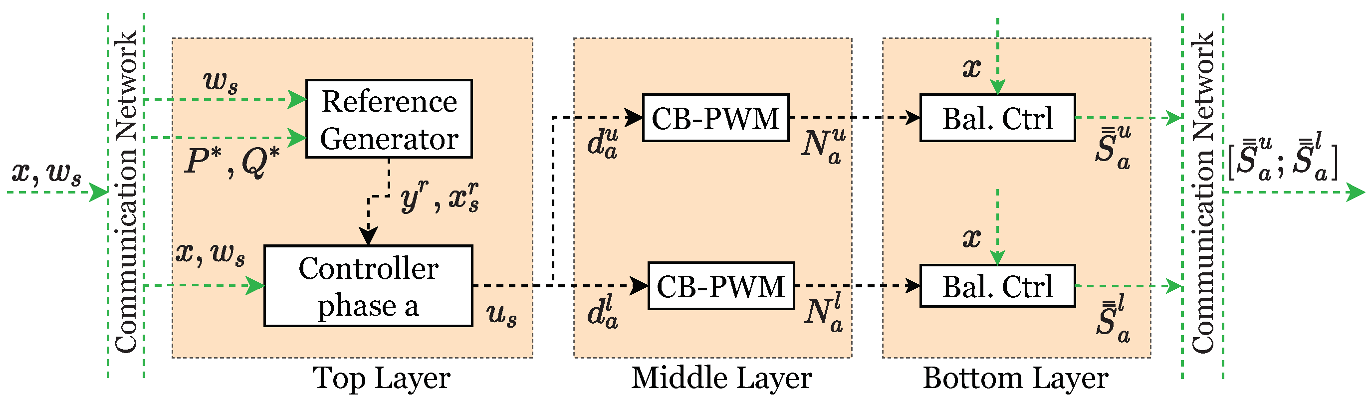
3.1. Standard Control Scheme for MMCs

In control of MMCs, a standard three-layer hierarchical control scheme is used; see Figure 3 [9]. In the top layer, a current controller uses the information from model (38) to control the output current, the average capacitor voltage, and the circulating current. As it is seen in Figure 3, the “Controller phase a” block receives the references for the output current, circulating current, and capacitor voltages from a Reference Generator block. The control signals computed by the current controller (a long-horizon NMPC controller in this paper) are real-valued insertion indexes $(d_m^r)$, which are set as the voltage references for the CB-PWM in the middle layer. In the middle layer, the CB-PWM translates the insertion index $(d_m^r)$ into integer variables $N_m^r$ that indicate how many submodules need to be switched ON or OFF. For this paper, multilevel CB-PWM as in [28] is used.

At the bottom layer, each arm employs an independently operating controller to balance the capacitor voltages by deciding on the switching signal $\left({\overline{S}}^{r,m}\right)$ for the individual submodules. The control signals of the bottom layer balancing controllers are the gating commands for the entire arm defined as ${\overline{\overline{S}}}_m^r:={\left[{\overline{S}}_1^{r,m}\dots {\overline{S}}_N^{r,m}\right]}^{\top }$. The basic principle for this approach is to order the charging and discharging of the submodules capacitors based on the arm current direction and the instantaneous value of the capacitor voltage. For the positive direction of the arm current, capacitors with the lowest voltage are inserted in the arm for maintaining all the voltage from the capacitors submodules around the same value. The opposite is done if the arm current direction is negative. The interested reader is referred to [9] for more details.

3.2. Control Objectives

The main task of the MMC is to control the power transfer between the grid and the DC bus. For this system, the instantaneous power in the grid side is described as

$$\begin{array}{cc}\hfill P_{AC}& =v_a^g{i}_a+v_b^g{i}_b+v_c^g{i}_c,\hfill \end{array}$$

(21)

$$\begin{array}{cc}\hfill Q_{AC}& =\frac{1}{\sqrt{3}}(v_a^g{i}_a+v_b^g{i}_b+v_c^g{i}_c),\hfill \end{array}$$

(22)

where $P_{AC}$ and $Q_{AC}$ are the active and reactive power on the grid side. The active power in the DC-bus $(P_{DC})$ is defined as

$$P_{DC}=2i_{DC}·v_{DC}.$$

(23)

To guarantee a proper and safe functioning of each of the phase $m\in \{a,b,c\}$ of the MMC, four variables are controlled: the output current $(i_m)$, the circulating current $(i_m^z)$, the upper average capacitor voltage $\left(v_{u,m}^{\Sigma }\right)$, and the lower average capacitor voltage $\left(v_{l,m}^{\Sigma }\right)$ [9,10].

Equations (21) and (22) show how the grid voltage and the output current determine the power extracted from the grid. Therefore, for assuring the desired power transfer, a tracking problem is formulated, such that

$$\underset{t\to \infty }{lim}|y_1(t)-y_1^r(t)|=0,$$

(24)

where $y_1(t)=i_m(t)$ and the reference for the output current $y_1^r(t):=i_m^r(t)$ for each phase $m\in \{a,b,c\}$ can be calculated with (21) and (22). However, as this is an undetermined system of equations, using the amplitude-invariant Clarke transformation, a determined system of equations is used instead, i.e.,

$$\left[\begin{array}{c}{i}_{\alpha }^{*}(t)\\ i_{\beta }^{*}(t)\end{array}\right]=\frac{2}{v_{\alpha }^2(t)+v_{\beta }^2(t)}\left[\begin{array}{cc}{v}_{\alpha }(t)& v_{\beta }(t)\\ v_{\beta }(t)& -v_{\alpha }(t)\end{array}\right]\frac{1}{3}\left[\begin{array}{c}{P}_{\mathrm{AC}}^{*}(t)\\ Q_{\mathrm{AC}}^{*}(t)\end{array}\right],$$

(25)

where $v_{\alpha }$ and $v_{\beta }$ are the transformation of $v_m^g$ in the $\alpha \beta$ coordinates, and $P_{\mathrm{AC}}^{*}$ and $Q_{\mathrm{AC}}^{*}$ are the desired active and reactive power on the grid side. Hence, the output current reference is obtained applying the inverse of the amplitude-invariant Clarke transformation, such that

$$\left[\begin{array}{c}{i}_a^r(t)\\ i_b^r(t)\\ i_c^r(t)\end{array}\right]=\frac{3}{2}\left[\begin{array}{cc}\frac{2}{3}& 0\\ -\frac{1}{3}& \frac{\sqrt{3}}{3}\\ -\frac{1}{3}& -\frac{\sqrt{3}}{3}\end{array}\right]\left[\begin{array}{c}{i}_{\alpha }^{*}(t)\\ i_{\beta }^{*}(t)\end{array}\right].$$

(26)

Using (25) also guarantees low THD if the reference is tracked accurately. Additionally, the output current is limited to reduce THD and grid interference as follows:

$$i_{min}\le y_1(t)\le i_{max},$$

(27)

where $i_{max}$ and $i_{min}$ are the upper and lower limit of the output current.

The reliability of the MMC depends on the capacity of rejecting both exogenous inputs, the grid and the DC-bus voltage. That is possible if $v_{r,m}^{\Sigma }(t)\ge \left|v_m^g(t)\right|+v_{DC}$. For this application, the nominal average capacitor voltage $({\overline{v}}^{\Sigma })$ is set such that

$${\overline{v}}^{\Sigma }=v_{DC}+{\widehat{v}}_m^g,$$

(28)

where ${\widehat{v}}_m^g$ is the peak of the grid phase voltage. This ensures reliability and reduces the capacitance needed for designing an MMC suitable for the application. Therefore, the control objective for the average capacitor voltage is formulated as

$$\begin{array}{c}\hfill \underset{t\to \infty }{lim}|x_{s,3}(t)-{\overline{v}}^{\Sigma }|\le {\delta }_{\Sigma },\end{array}$$

(29a)

$$\begin{array}{c}\hfill \underset{t\to \infty }{lim}|x_{s,4}(t)-{\overline{v}}^{\Sigma }|\le {\delta }_{\Sigma },\end{array}$$

(29b)

where $x_{s,3}(t)=v_{u,m}^{\Sigma }(t)$, $x_{s,4}(t)=v_{l,m}^{\Sigma }(t)$, and ${\delta }_{\Sigma }$ is a bound determined by the user and the application. Additionally, limits are imposed on the capacitor voltages as follows:

$$\begin{array}{c}\hfill v_{min}^{\Sigma }\le x_{s,3}(t)\le v_{max}^{\Sigma },\end{array}$$

(30a)

$$\begin{array}{c}\hfill v_{min}^{\Sigma }\le x_{s,4}(t)\le v_{max}^{\Sigma },\end{array}$$

(30b)

where $v_{max}^{\Sigma }={\overline{v}}^{\Sigma }+{\delta }_{\Sigma }$ and $v_{min}^{\Sigma }={\overline{v}}^{\Sigma }-{\delta }_{\Sigma }$ are the upper and lower limit of the average capacitor voltage. It is important to observe that regardless of the application, ${\delta }_{\Sigma }>0$ because for (24) to hold, then $v_{r,m}^{\Sigma }(t)$ cannot be constant. Hence, these control objectives are competing and cannot be satisfied simultaneously.

Ideally, $i_m^{\Sigma }=i_{DC}$, since the common-mode current is the inner current flowing through the arm and the DC-bus components. Hence, $i_m^{\Sigma }(t)=i_{DC}(t)$ means that the MMC achieves 100% efficiency. However, due to the conduction and devices losses represented by $R_m$, this is not achievable. To control the efficiency of the system, a new inner current for each leg, called the circulating current $(i_m^z)$, is defined, such that

$$i_m^z(t)=\frac{1}{2}(i_m^u(t)+i_m^l(t))-\frac{1}{3}{i}_{DC},$$

(31)

which is only true if the grid and the MMC are balanced. In [29,30], it is proven that the steady state of the common-mode current only has even harmonics, such that it can be defined as

$$i_m^{\Sigma }=\frac{1}{3}{i}_{DC}+{\widehat{I}}_m^{\Sigma }cos\left(h·2\pi f_g·t+{\varphi }_2\right),\forall h=2k,k\in \mathbb{N},$$

(32)

where $f_g$ is the grid frequency, ${\widehat{I}}_m^{\Sigma }$ and ${\varphi }_2$ are the amplitude and the phase of the common-mode current. Substituting (32) in (31), the circulating current is defined as

$$i_m^z={\widehat{I}}_m^{\Sigma }cos\left(h·2\pi f_g·t+{\varphi }_2\right).$$

(33)

Re-arranging the power balance equation of the system, the amplitude of the common-mode current is formulated as

$${\widehat{I}}_m^{\Sigma }=\sqrt{-\frac{{\widehat{v}}_m^g·{\widehat{i}}_m}{2R_m}cos(\varphi )-\frac{{\widehat{i}}_m^g{}^2}{4}-2\frac{{i_{DC}}^2}{9}+\frac{v_{DC}·i_{DC}}{3R_m}},$$

(34)

where $\varphi$ is the phase difference between the current and voltage of the grid. In this paper, the efficiency $(\eta )$ of the MMC is defined by its capacity of transferring power, such that $\eta =P_{DC}/P_{AC}$. Hence, using (34), a relationship between the amplitude of the common-mode current and the efficiency of the MMC is established. For ensuring a desired level of efficiency, the control objective for the circulating current is formulated as

$$\underset{t\to \infty }{lim}|y_2(t)-y_2^r(t)|=0,$$

(35)

where $y_2(t)=i_m^{\Sigma }(t)$ and $y_2^r(t):=\frac{1}{3}{i}_{DC}(t)$. Similarly as above, we also impose limits on the circulating current as follows:

$$i_{min}^z\le y_2(t)\le i_{max}^z,$$

(36)

where $i_{max}^z={\widehat{I}}_m^{\Sigma }$ and $i_{min}^z=-{\widehat{I}}_m^{\Sigma }$ are the upper and the lower limit of the circulating current. As the highest efficiency possible is determined by $R_m$, the minimal achievable circulating current is also limited by this element.

Observe also that suppressing the circulating current forces the common-mode current to be close to a defined value meaning that the average of the arm current is also regulated. Since the MMC power losses $(P_{losses})$ can be defined as

$$P_{losses}=R_m·{\left(i_{m_{RMS}}^u\right)}^2+R_m·{\left(i_{m_{RMS}}^l\right)}^2,$$

(37)

see [7] for details, controlling the circulating current keeps the power losses as low as possible.

In summary, the current controller, i.e., the NMPC controller to be designed, has to track a time-varying sinusoidal reference for the output current, which is known in advance over the prediction horizon, to track a time-varying reference for the circulating current, which is assumed constant over the prediction horizon, and to keep the capacitor voltages as close as possible to their nominal value, without sacrificing the tracking performance. All these objectives must be achieved subject to soft constraints and hard constraints, which will be defined in the next section.

4. Nonlinear Model Predictive Control Design and Implementation

The NMPC scheme proposed in this paper follows the principle of receding horizon optimal control. In this case, at each sampling instant k, given the current state $x_s(k)$, an optimization problem is formulated and solved in real time. As a result, an optimal (or feasible) sequence of control inputs $U(k)=\left[u_{0|k},u_{1|k},\dots ,u_{N_p-1|k}\right]$ is obtained for a prediction horizon $N_p$, which is optimal on the basis of a cost function subject to the dynamics of the prediction model and constraints. Following the receding horizon policy, only the first input $u_s(k):=u_{0|k}$ in the sequence is applied to the system, and the process is repeated at the next sampling instant $k+1$. Additionally, if soft constraints are implemented, the optimization problem needs to find a sequence of slack variables $\mathcal{E}(k)=\left[{\overline{\epsilon }}_{0|k},{\overline{\epsilon }}_{1|k},\dots ,{\overline{\epsilon }}_{N_p-1|k}\right]$, which penalize violation of the soft constraints, see, e.g., [31].

In consonance with the analysis in Section 2.2, the prediction model used is the discrete-time bilinear model (19), i.e.,

$$\begin{array}{cc}\hfill x_{i+1|k}& =A_d(u_{i|k})x_{i|k}+D_d{w}_{i|k},\hfill \\ \hfill y_{i|k}& =C_c{x}_{i|k},\forall i=\{0,\dots ,N_p-1\},\hfill \end{array}$$

(38)

where $x_{i|k}$, $u_{i|k}$, and $w_{i|k}$ denote the predicted state, control input, and exogenous input vectors at i-steps in the future, starting from the current system state $x_s(k)$ and exogenous input vector $w_s(k)$measured at time k. Note that $i\in \mathbb{N}$, $i=0,1,\dots ,N_p-1$ and $N_p$ is the prediction horizon. The prediction model and real system states and inputs are linked for all $k\in {\mathbb{Z}}_{+}$ via the relations $x_{0|k}:=x_s(k)$, $u_s(k):=u_{0|k}$. Additionally, $w_{i|k}$ is determined as follows: for the grid voltage, we assume perfect knowledge along the prediction horizon, due to its periodic nature, and for the DC voltage and DC current, we keep the measured values at time k constant over the prediction horizon.

As explained in the previous Section 3.2, the MMC control problem is a constrained control problem due to the operation characteristics of the MMC. In this paper, not all the constraints were catalogued the same. Based on the control objectives definitions, (27), (30a), (30b), and (36) are treated as soft constraints since they are only performance requirements. Moreover, the system also has hard constraints due the physical limitations of the MMC, such as continuous insertion index, which it is limited by

$$\begin{array}{cc}\hfill -1& \le d_{m_{i|k}}^u\le 1,\forall i=\{0,\dots ,N_p-1\},\hfill \end{array}$$

(39a)

$$\begin{array}{cc}\hfill -1& \le d_{m_{i|k}}^l\le 1,\forall i=\{0,\dots ,N_p-1\},\hfill \end{array}$$

(39b)

where $d_{m_{i|k}}^u$ and $d_{m_{i|k}}^l$ form the predicted input vector $u_{i|k}$. The voltage of the polarized capacitors is also limited as follows

$$\begin{array}{cc}\hfill 0& \le v_{u,m_{i|k}}^{\Sigma },\forall i=\{0,\dots ,N_p-1\},\hfill \end{array}$$

(40a)

$$\begin{array}{cc}\hfill 0& \le v_{l,m_{i|k}}^{\Sigma },\forall i=\{0,\dots ,N_p-1\}.\hfill \end{array}$$

(40b)

In this paper, it is assumed that grid components $R_g$ and $L_g$ are small enough to be disregarded. Moreover, $P_{DC}$ behaves as a piece-wise step function with a constant voltage during the entire simulation. Hence, the derivative of the DC-bus current is assumed equal to zero.

Cost Function and Optimization Problem

The cost function is a scalar mapping of the desired performance of the control objectives. A crucial criterion for developing a tracking MPC is that the number of tracked output needs to be less than or equal to the number of control inputs. Hence, in this case, only two outputs can be accurately tracked.

The multiple control objectives of the MMC compete among them; therefore, it is impossible to find a control sequence that gives the optimal solution for all control objectives simultaneously. Hence, aiming to achieve Pareto optimal performance, a cost function is defined as

$$J(x(k),u(k-1),\mathcal{E}(k),U_k):=J_1(k)+J_2(k)+J_3(k),$$

(41)

where the individual cost functions are defined next. Firstly, for solving the tracking problem of the output current and suppressing the circulating current, the cost function $J_1$ is formulated as

$$J_1(x(k),u(k-1),U(k))=\sum _{i=0}^{N_p-1}\left({∥y_{i|k}-y_{i|k}^r∥}_{Q_1}^2+{∥\Delta u_{i|k}∥}_R^2\right),$$

(42)

where $Q_1\in {\mathbb{R}}^{2\times 2}$ contains the weighting factors that penalize the tracking error and the deviation of the circulating current, $R\in {\mathbb{R}}^{2\times 2}$ penalizes the control input rate of change $\Delta u_{i|k}:=u_{i|k}-u_{i-1|k}$ for $i=0,\dots ,N_p-1$ ($u_{-1|k}:=u(k-1)$), and $y_{i|k}^r={\left[{y_1^r}_{i|k}{y_2^r}_{i|k}\right]}^{\top }$ denotes the time-varying output reference vector, which is computed as explained in the previous section.

Secondly, the cost function $J_2$ aims to keep the average capacitor voltage near to a desired nominal as follows

$$J_2(x(k),U_k)=\sum _{i=0}^{N_p-1}{∥x_{i|k}^{\{3,4\}}-x_{i|k}^{{\{3,4\}}^r}∥}_{Q_2}^2,\forall i=\{0,\dots ,N_p-1\},$$

(43)

where $x_{i|k}^{\{3,4\}}={\left[v_{{u,m}_{i|k}}^{\Sigma }{v}_{{l,m}_{i|k}}^{\Sigma }\right]}^{\top }$, $Q_2\in {\mathbb{R}}^{2\times 2}$ contains the weighting factors for penalizing the average capacitor voltage deviations and $x_{i|k}^{{\{3,4\}}^r}:={\left[{\overline{v}}^{\Sigma }{\overline{v}}^{\Sigma }\right]}^{\top }$ is the vector containing the nominal value of the average capacitor voltages. Since the MMC of UFCSs operates in an extended region, the standard formulation of the nominal value, see e.g., [2,32], does not ensure the desired performance. Therefore, the nominal average capacitor voltage is set as (28) for guaranteeing proper sizing of the capacitance and keeping the energy stored in the MMC balanced.

Thirdly, to implement soft constraints for (27), (30a,b), and (36), we define the slack variable vector $\overline{\epsilon }:={\left[{\epsilon }^1,{\epsilon }^2,{\epsilon }^3,{\epsilon }^4\right]}^{\top }\in {\mathbb{R}}_{+}^4$ and the cost function

$$J_3({\mathcal{E}}_k)=\sum _{i=0}^{N_p-1}\lambda \left|\right|{\overline{\epsilon }}_{i|k}{\left|\right|}_1,$$

(44)

where ${\epsilon }^1$, ${\epsilon }^2$, ${\epsilon }^3$, and ${\epsilon }^4$ are slack variables that penalize the constraints violation of the output current, upper average capacitor voltage, lower average capacitor voltage, and circulating current, and $\lambda$ is a constant that penalizes the slack variables and determines how strict the soft constraints are [31,33]. The corresponding soft constraints are defined as follows:

$$\begin{array}{cc}\hfill {\epsilon }_{i|k}^1& \ge 0,\hfill \end{array}$$

(45a)

$$\begin{array}{cc}\hfill {\epsilon }_{i|k}^1& \ge i_{m_{i|k}}-i_{max},\hfill \end{array}$$

(45b)

$$\begin{array}{cc}\hfill {\epsilon }_{i|k}^1& \ge -(i_{m_{i|k}}-i_{min}),\forall i=\{0,\dots ,N_p-1\}.\hfill \end{array}$$

(45c)

Similarly, the average capacitor voltage constraints are reformulated. For the upper and lower average capacitor voltage (30a,b) respectively, the new inequalities are

$$\begin{array}{cc}\hfill {\epsilon }_{i|k}^2& \ge 0,{\epsilon }_{i|k}^3\ge 0,\hfill \end{array}$$

(46a)

$$\begin{array}{cc}\hfill {\epsilon }_{i|k}^2& \ge v_{u,m_{i|k}}^{\Sigma }-v_{\max }^{\Sigma },{\epsilon }_{i|k}^3\ge v_{l,m_{i|k}}^{\Sigma }-v_{\max }^{\Sigma },\hfill \end{array}$$

(46b)

$$\begin{array}{cc}\hfill {\epsilon }_{i|k}^2& \ge -(v_{u,m_{i|k}}^{\Sigma }-v_{\min }^{\Sigma }),{\epsilon }_{i|k}^3\ge -(v_{l,m_{i|k}}^{\Sigma }-v_{\min }^{\Sigma }),\forall i=\{0,\dots ,N_p-1\}.\hfill \end{array}$$

(46c)

The circulating current constraints are reformulated as

$$\begin{array}{cc}\hfill {\epsilon }_{i|k}^4& \ge 0,\hfill \end{array}$$

(47a)

$$\begin{array}{cc}\hfill {\epsilon }_{i|k}^4& \ge i_{m_{i|k}}^z-i_{\max }^z,\hfill \end{array}$$

(47b)

$$\begin{array}{cc}\hfill {\epsilon }_{i|k}^4& \ge -(i_{m_{i|k}}^z-i_{\min }^z),\forall i=\{0,\dots ,N_p-1\}.\hfill \end{array}$$

(47c)

Using (41), the NMPC algorithm for MMCs is formulated as the following optimization problem:

$$\begin{array}{ccc}\hfill \underset{U(k),\mathcal{E}(k)}{min}& J(x(k),u(k-1),\mathcal{E}(k),U(k))\hfill & \end{array}$$

(48a)

$$\begin{array}{cc}\hfill & \mathrm{s}.\mathrm{t}.x_{i+1|k}=A_d(u_{i|k})x_{i|k}+D_d{w}_{i|k},\hfill \end{array}$$

(48b)

$$\begin{array}{cc}\hfill & -1\le d_{m_{i|k}}^u\le 1,-1\le d_{m_{i|k}}^l\le 1,\hfill \end{array}$$

(48c)

$$\begin{array}{cc}\hfill & v_{u,m_{i|k}}^{\Sigma }\ge 0,v_{l,m_{i|k}}^{\Sigma }\ge 0,\hfill \end{array}$$

(48d)

$$\begin{array}{cc}\hfill & {\epsilon }_{i|k}^1\ge 0,{\epsilon }_{i|k}^2\ge 0,{\epsilon }_{i|k}^3\ge 0,{\epsilon }_{i|k}^4\ge 0,\hfill \end{array}$$

(48e)

$$\begin{array}{cc}\hfill & {\epsilon }_{i|k}^1\ge i_{m_{i|k}}-i_{max},{\epsilon }_{i|k}^2\ge v_{u,m_{i|k}}^{\Sigma }-v_{\max }^{\Sigma },\hfill \end{array}$$

(48f)

$$\begin{array}{cc}\hfill & {\epsilon }_{i|k}^3\ge v_{l,m_{i|k}}^{\Sigma }-v_{\max }^{\Sigma },{\epsilon }_{i|k}^4\ge i_{m_{i|k}}^z-i_{\max }^z,\hfill \end{array}$$

(48g)

$$\begin{array}{cc}\hfill & {\epsilon }_{i|k}^1\ge -(i_{m_{i|k}}-i_{min}),{\epsilon }_{i|k}^2\ge -(v_{u,m_{i|k}}^{\Sigma }-v_{\min }^{\Sigma }),\hfill \end{array}$$

(48h)

$$\begin{array}{cc}\hfill & {\epsilon }_{i|k}^3\ge -(v_{l,m_{i|k}}^{\Sigma }-v_{\min }^{\Sigma }),{\epsilon }_{i|k}^4\ge -(i_{m_{i|k}}^z-i_{\min }^z),\hfill \end{array}$$

(48i)

$$\begin{array}{cc}\hfill & \forall i=\{0,\dots ,N_p-1\}.\hfill \end{array}$$

(48j)

For solving the Nonlinear Programming (NLP) problem (48a) subject to (48b–i), an efficient NMPC solver based on Sequential Quadratic Programming (SQP) [34] can be used. In this paper, the ACADO Toolkit NMPC solver from [22] was used in combination with the qpOASES Active Set QP solver [35].

Since the main objective is to speed up the solver, we changed the default ACADO configuration. In this case, the KKT tolerance was relaxed to ${10}^{-3}$ allowing a faster convergence. The Hessian approximation method used was the Gauss–Newton method. Compared to calculating Exact Hessian, this method represents a considerable time reduction, since there is no need for calculating second-order derivatives. The maximum number of iteration QP per sampling was set to 200, although as the KKT tolerance was softened, the maximum number of iterations should not be reached. In addition, the discretization type used was multiple shooting, since it provides a faster implementation.

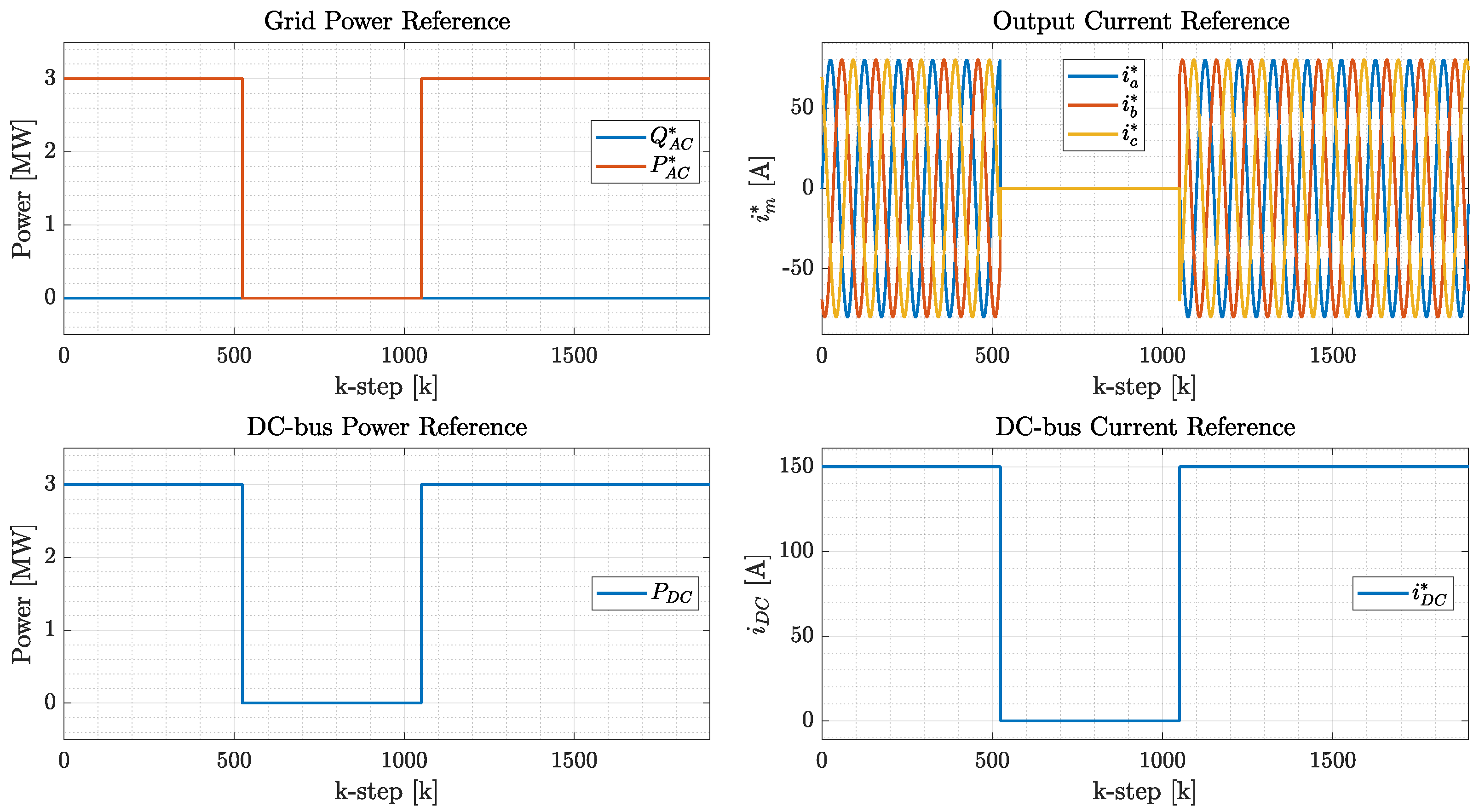
5. Case Study: Control of Modular Multilevel Converters for Ultra-Fast Charging Stations of Electric Vehicles

This section presents the results of testing the proposed controller in an ultra-fast charging station topolgy presented in [7]. The rest of this section contains a brief description of the UFCS topology and the simulations from three different scenarios. The first scenario shows the performance of the NMPC when long prediction horizons are implemented. The second scenario compares the NMPC and MPC using a long prediction horizon. Finally, the third scenario offers insightful information about what is gained from the proposed prediction model and cost function.

5.1. Ultra-Fast EV Charging Stations Topology

The proposed control solution is tested in the MMC topology for UFCSs presented in [6]. In this case, the nominal active power of the UFCS is 3 MW. The grid is considered three-phase with 25 kV phase voltage. The nominal DC-bus voltage is 10 kV. The simulations of the UFCS and their control elements were done in MATLAB/Simulink and PLECs.

Table 3. UFCS parameters from [6].

Component	Parameter	Symbol	SI Value
Grid	Frequency	$f_g$	50 Hz
Grid	Peak phase voltage	${\widehat{v}}_m^g$	25 kV
Grid	Nominal active power	${\overline{P}}_{AC}$	3 MW
DC Bus	DC Voltage	$v_{DC}$	10 kV
MMC	Arm resistance	$R_m$	50 m$\Omega$
MMC	Arm inductance	$L_m$	3 mH
MMC	Capacitance	C	4 mF
MMC	Number of SMs	N	4

depicts more information about the UFCS components.

The control scheme used follows the guidelines explained in Section 3.1. In this case, at the Top layer, an NMPC (or linearization-based) MPC algorithm is used. The weighting factors were defined as $Q_1=\mathrm{diag}(1500,1500)$, $Q_2=\mathrm{diag}(10,10)$ $R=\mathrm{diag}(1,1)$, and $\lambda ={10}^5$. To put more emphasis on tracking performance, $Q_1$ has a much higher value than $Q_2$. The high value of $\lambda$ is meant to strictly penalize the violation of soft constraints, as this improves the performance and efficiency of the MMC. The limits used in hard and soft constraints are provided in

Table 4. Limits used in the system constraints.

	Variable
Limit	${\mathit{i}}_{\mathit{m}}$	${\mathit{v}}_{\mathit{r},\mathit{m}}^{\Sigma }$	${\mathit{i}}_{\mathit{m}}^{\mathit{z}}$	${\mathit{d}}_{\mathit{m}}^{\mathit{r}}$
Upper	1.1 $\times max\left(|i_m^{*}|\right)$	1.2$·{\overline{v}}^{\Sigma }$	$0.1i_{DC}$	1
Lower	−1.1 $\times max\left(|i_m^{*}|\right)$	0.8$·{\overline{v}}^{\Sigma }$	$-0.1i_{DC}$	−1

.

At the middle layer, a regularly sampled multilevel CB-PWM with phase disposition is used with a carrier frequency of 2.5 KHz. At the bottom layer, the balancing control from [9] is implemented.

Checking the performance of the MMC, a transient test is carried out. In Figure 4, the desired power extracted from the grid and the corresponding output current reference are depicted. In this case, a full power transfer is expected, and based on that, the desired DC-bus current is calculated; see Figure 4.

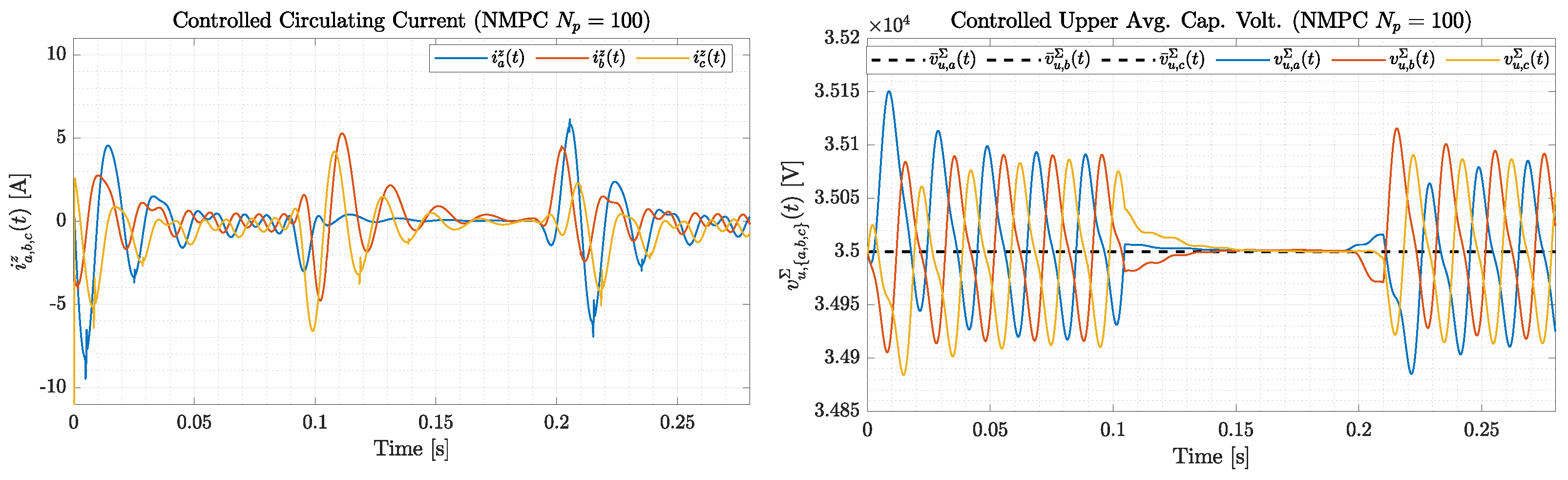
5.2. Results for NMPC with $N_p=100$

Figure 5 presents the behavior of the output current controlled with the NMPC using $N_p=100$. In this case, the NMPC scheme manages to regulate the output current closely along the references presented in Figure 4. The proposed control solution reaches the expected steady state, such as the one in [7], at a high speed without affecting other performance indexes. The average mean square error (MSE) among the three phases is $0.26$, and the THD of the output current equals is $0.11$%, which proves the good performance of long-horizon NMPC.

The remaining controlled variables show an adequate behavior; see Figure 6. During this test, the constraints are not violated, and the controlled variables are kept near the references. The different behavior among the phases is mainly due to the initial conditions chosen. For this test, all phase legs have the same initial states but the references are not the same for every phase. Regardless, the performance of all phases is suitable. For the average capacitor voltage, the mean deviation with respect to the nominal voltage is approximately 7 V and the standard deviation error is 56.58 V which represent less than 0.16% of the nominal value. Finally, the root mean square (RMS) of the circulating current is approximately 1.3 A, which is less than 0.2%.

One of the main advantages of using MPC is faster convergence to the steady state and consequently shorter settling time $(T_{sett})$. In

Table 5. Performance comparison of the NMPC for the phase a with different $N_p$.

			Computational Time [ms]
${\mathit{N}}_{\mathit{p}}$	THD$({\mathit{i}}_{\mathit{a}})$ [%]	${\mathit{T}}_{\mathit{sett}}$ [s]	Mean	Std	Max	Min
$N_p=10$	0.46	≈0.35	0.11	0.02	0.25	0.092
$N_p=25$	0.21	≈0.22	0.13	0.021	0.22	0.109
$N_p=50$	0.053	≈0.17	0.28	0.036	0.49	0.23
$N_p=100$	0.036	≈0.1	1.3	0.156	2.2	1.09

, performance indicators are provided for various values of the prediction horizon. These indicators show that using a gradually longer prediction horizon corresponds to gradually increasing the performance and efficiency, which was matched by a reasonable increase in the required computation time. Among the considered indicators are also the mean, the standard deviation (std), the maximum (max), and the minimum (min) of the computational time, since the suitability of this method for real-time implementation is investigated.

Based on Table 5, $N_p=25$ is already compatible with real-time implementation for a sampling period $T_s=0.2$ ms. For the remaining prediction horizons, it is key to clarify that the developed NMPC algorithm was implemented using the ACADO Toolkit on a 2.59 GHz Intel Core-i7-9750H using the MATLAB interface. On the other hand, in power electronic applications, controllers are implemented in real time using special hardware, such as field-programmable gate array (FPGA) and digital signal processors (DSP). FPGAs significantly outperform microprocessor and DSP implementations due to their parallelism characteristic [24]. As observed in [36], it is expected that FPGAs have a computational time 10 times shorter than the microprocessor implementations. This time reduction increases if the state dimension and prediction horizon increase [36]. Aligned with the results of [36], in [37], a nonlinear MPC with a long prediction horizon for Interleaved Switching AC/DC converters was tailored in an FPGA. In that case, the computational time was around 10 $\mathsf{\mu }$s when a prediction horizon of 100 was used. Hence, using an FPGA will speed up our solves so that real-time implementation for $N_p=100$ will be feasible. Moreover, unlike other voltage-source converters, MMCs operate at low frequencies without significantly decreasing their performance. Hence, it is possible to decrease the carrier frequency/the sampling period up to certain limits [18].

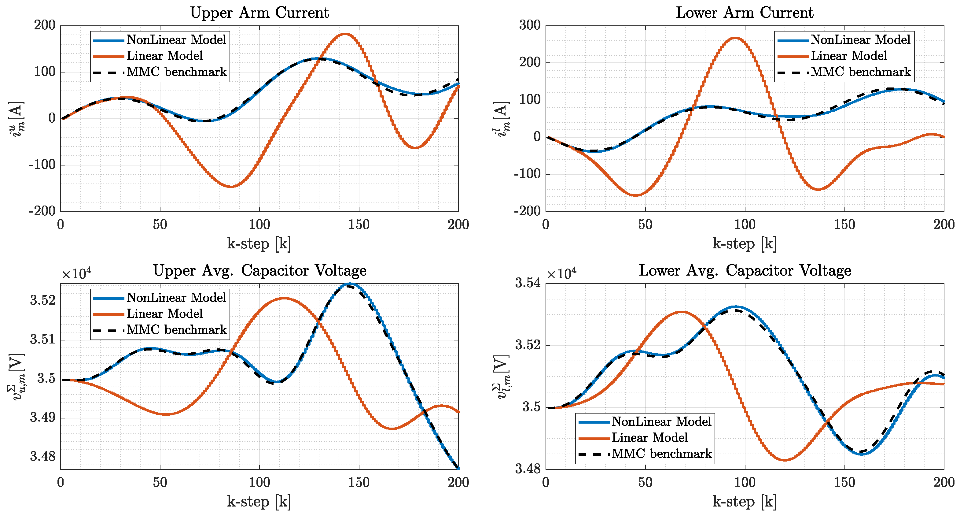
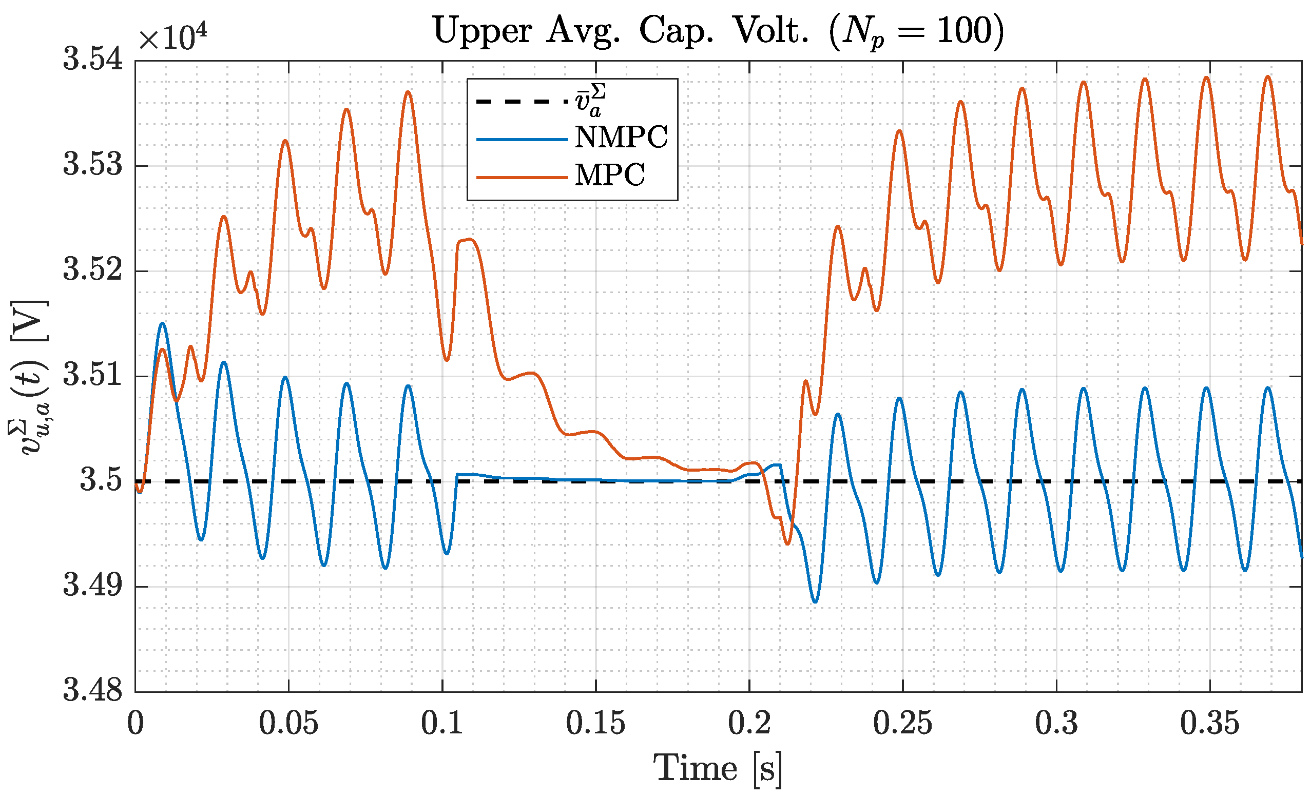
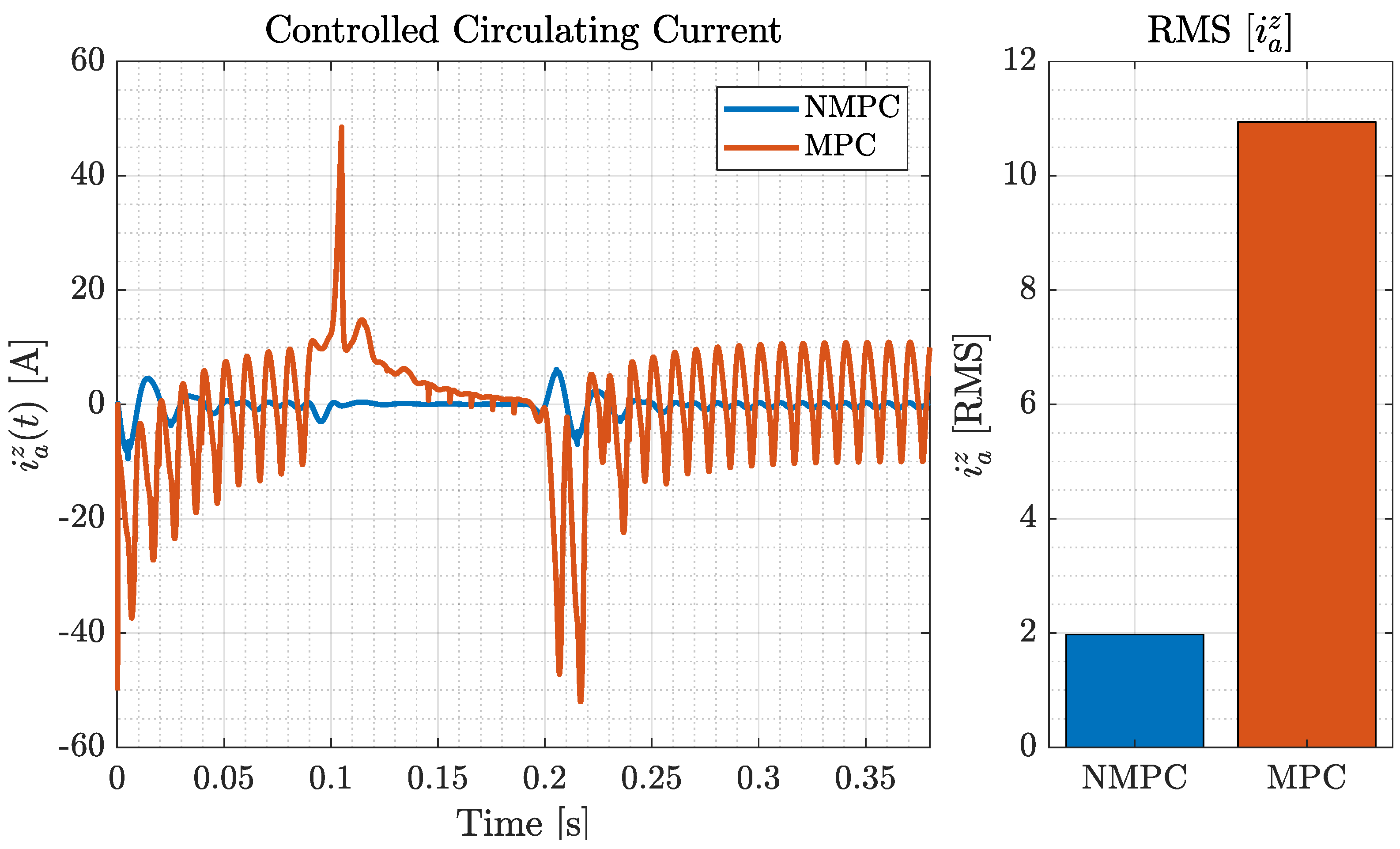
5.3. NMPC vs. Linearization-Based MPC Comparison for $N_p=100$

Conversely to the behavior observed in NMPC implementation, when longer prediction horizons are used in a linearization-based MPC formulation, the performance of the MMC decreases significantly. These results are aligned with the findings from the model validation. The upper and lower limits of the output current are reached when the linearization-based MPC is used. Due to the soft constraints, these limits are not violated; see Figure 7. However, the observed performance is not suitable for the application.

In the case of the average capacitor voltage, the limits are not reached. However, conversely to the NMPC performance, the voltage does not oscillate around the nominal value; see Figure 8. The comparison with the NMPC behavior shows an increase in the average deviation to the nominal average capacitor voltage and an increase in the standard deviation.

The circulating current performance shows a significant difference compared to the NMPC; see Figure 9. The observed behavior of the circulating current is unsuitable for this application due to the high amplitude of the oscillations of the circulating current. Moreover, the current peaks are harmful to the MMC component lifespan. The evidenced behavior of the circulating current could endanger the safe functioning and the lifetime of the MMC. This increase in the circulating current is directly reflected in the arm current and, consequently, in the MMC losses. When the linearization-based MPC is used, the losses increase by 6.8%.

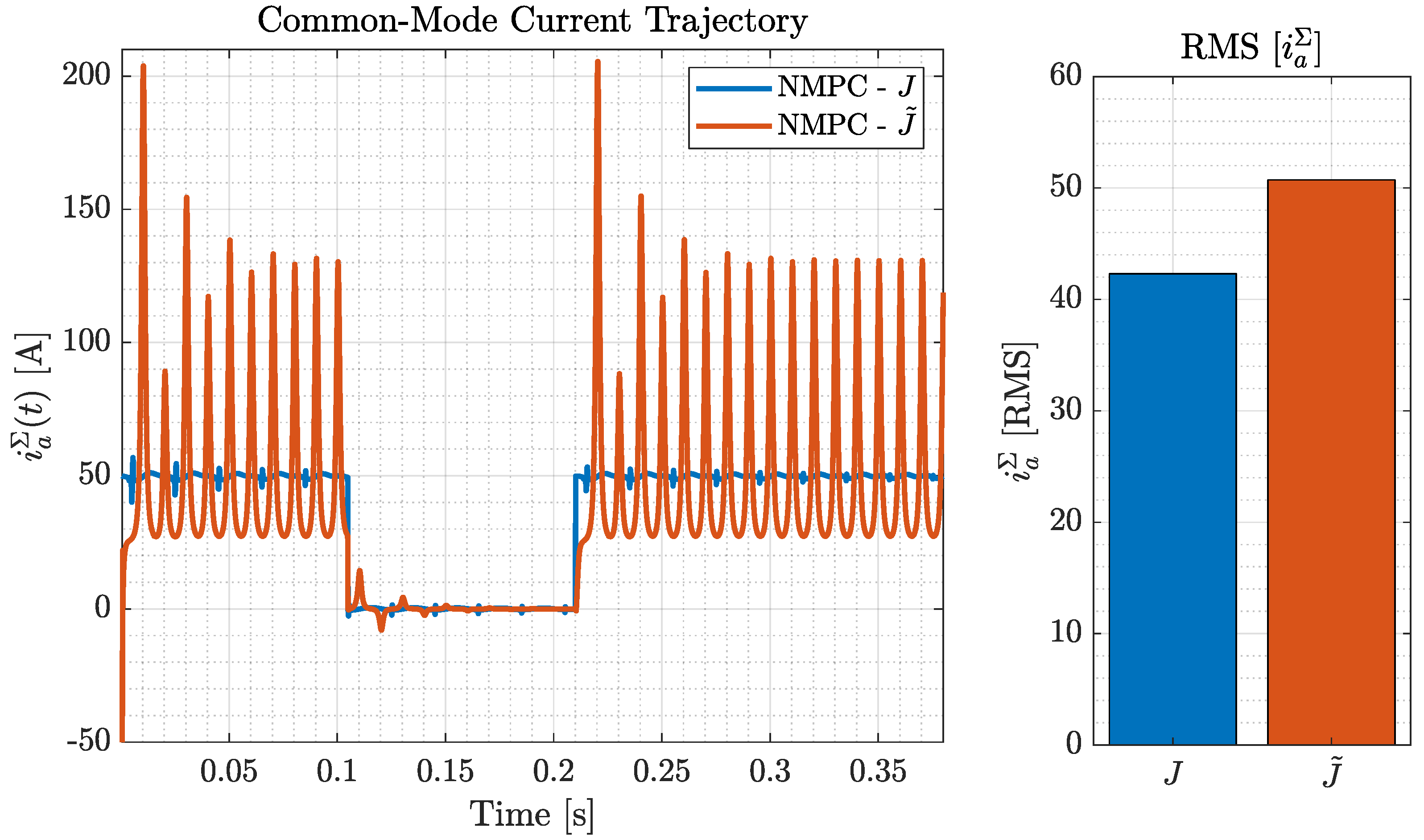
5.4. Evaluation of the NMPC Cost Function

In this paper, a different prediction model and corresponding cost function were derived, which enabled directly controlling the circulating current. To assess the benefits of penalizing the circulating current in the cost function, even for a short prediction horizon, we compare the proposed NMPC algorithm for $N_p=10$ (as used in [18]) with the following cost functions: (i)—the cost function (41) developed in this paper and (ii)—a cost function that mimics the cost function derived in [2], denoted as $\tilde{J}$, for the prediction model (19). The cost function $\tilde{J}$ is obtained by taking the output of model (19) as the output current and the capacitor voltages, and then adding the correspond ${\tilde{J}}_1$ and ${\tilde{J}}_3$ costs (i.e., corresponding to $J_1$ and $J_3$ for the redefined output). The main difference is that the cost function ${\tilde{J}}_1$ corresponding to $J_1$ does not penalize the circulating current and that the cost ${\tilde{J}}_1$ penalizes the capacitor voltages as well, so the cost $J_2$ is no longer used.

Figure 10 depicts the trajectory of the circulating current corresponding to the above-mentioned cost functions. When the circulating current is not penalized, extremely high peaks are observed. The RMS of the circulating current is significantly higher when the circulating current is not controlled. These results are similar to the findings in [2]. Consequently, in [38], which is continuation of the work of [2], the circulating current was controlled using an external PI controller to improve performance.

Penalizing the circulating current provides a 29.75% reduction of the power losses, and therefore, the efficiency increases. Figure 11 shows the behavior of the common-mode current, which determines the power losses. Since the control objectives compete among them, this increase of the circulating current amplitude allows an improvement in the behavior of the average capacitor voltage; see Figure 12. However, the improvement of the average capacitor voltage does not compensate for the high circulating current.

6. Discussion

The use of NMPC provides a significant improvement in the MMC control. These improvements are obtained mainly since nonlinear models can predict the MMC bilinear behavior. Using NMPC controllers, MMCs can be used in applications where more strict performance requirements are needed or the system properties demand a more accurate controller. Moreover, Figure 6 shows how the NMPC maintains the average capacitor voltage within 1% of the nominal value. Since the common indications for the constraints of the average capacitor voltage are a maximum deviation of approximately 20% of the nominal value, using NMPC enables the reduction of the capacitance of the submodule and, consequently, decreases the MMC cost. The faster convergence to a steady state makes the NMPC more suitable for applications such as UFCS stations, where quick changes on the setpoint during intense periods of operation are expected.

However, there are many challenges that the NMPC implementation needs to overcome in the future. The need for faster solvers is a constant challenge for MPC solutions. Even if in this application a real-time implementation is achievable, many MMC applications work at a higher frequency. Other improvements for the NMPC are providing some guarantees for stability and recursive feasibility. In this regard, we have to recall that our tracking problem has competing objectives and with less control inputs than output variables; therefore, minimizing the design cost function yields a Pareto-optimal solution. Methods for analyzing and providing some practical and robust stability for tracking MPC are presented in [39,40,41]. Exploring if these methods could be applied to our case is a good consideration for future works. In our application, we noted that using a long horizon is beneficial for stability. This observation aligns with the analysis on the stability of NMPC without terminal ingredients [42]. The other major challenge that the NMPC can encounter is the mismatches between the model and the real system due to uncertainties and perturbation of the grid or the failures in the lower control layers. Yet, this is a common challenge for the MPC solutions, and in this case, robust NMPC solutions can be studied to improve performance in conditions of high uncertainties.

7. Conclusions

A nonlinear model predictive control (NMPC) scheme for MMCs was proposed in this paper, which was motivated by the fact that linearization-based MPC for MMCs is limited to relatively short prediction horizons. The designed NMPC controller is suitable for various applications independently of the number of submodules of the MMC. Using a nonlinear prediction model enables a much larger prediction horizon (up to 100) compared to a linearized model (up to 10) and significantly increases perforamnce and efficiency. Using state-of-the-art in NMPC solvers based on sequential quadratic programming showed that the developed NMPC algorithm is suitable for real-time implementation with a long prediction horizon (ranging from 25 up to 100 with additional solver compiling and optimization) for a sampling period of $0.2$ ms. A new prediction model and cost function was developed that enables penalizing the circulating current, which resulted in significant power losses reduction and efficiency improvements. The efficiency and performance improvement brought by the developed NMPC control solution for MMCs was demonstrated in a case study from ultra-fast charging stations for electric vehicles.

References

1. Lesnicar, A.; Marquardt, R. An innovative modular multilevel converter topology suitable for a wide power range. In Proceedings of the 2003 IEEE Bologna Power Tech Conference Proceedings, Bologna, Italy, 23–26 June 2003; pp. 272–277. [Google Scholar]
2. Darivianakis, G.; Geyer, T.; van der Merwe, W. Model predictive current control of modular multilevel converters. In Proceedings of the 2014 IEEE Energy Conversion Congress and Exposition (ECCE), Pittsburgh, PA, USA, 14–18 September 2014; pp. 5016–5023. [Google Scholar]
3. Priya, M.; Ponnambalam, P.; Muralikumar, K. Modular-multilevel converter topologies and applications—A review. IET Power Electron. 2019, 12, 170–183. [Google Scholar] [CrossRef]
4. Ye, H.; Cao, W.; Chen, W.; Wu, H.; He, G.; Li, G.; Xi, Y.; Liu, Q. An AC Fault Ride Through Method for MMC-HVDC System in Offshore Applications Including DC Current-Limiting Inductors. IEEE Trans. Power Deliv. 2021. [Google Scholar] [CrossRef]
5. Martinez-Rodrigo, F.; Ramirez, D.; Rey-Boue, A.; De Pablo, S.; Herrero-de Lucas, L. Modular Multilevel Converters: Control and Applications. Energies 2017, 10, 1709. [Google Scholar] [CrossRef] [Green Version]
6. Marca, Y.P.; Roes, M.G.; Duarte, J.L.; Wijnands, K.G. Isolated MMC-based ac/ac stage for ultrafast chargers. In Proceedings of the 2021 IEEE 30th International Symposium on Industrial Electronics (ISIE), Kyoto, Japan, 20–23 June 2021; pp. 1–8. [Google Scholar] [CrossRef]
7. Pereira Marca, Y.; Duarte, J.; Roes, M.; Wijnands, C. Extended operating region of modular multilevel converters using full-bridge sub-modules. In Proceedings of the 23rd European Conference on Power Electronics and Application (EPE2021), Ghent, Belgium, 6–10 September 2021. [Google Scholar]
8. Lopez, A.; Quevedo, D.E.; Aguilera, R.; Geyer, T.; Oikonomou, N. Reference design for predictive control of modular multilevel converters. In Proceedings of the 2014 4th Australian Control Conference (AUCC), Canberra, ACT, Australia, 17–18 November 2014; pp. 239–244. [Google Scholar] [CrossRef]
9. Du, S.; Dekka, A.; Wu, B.; Zargari, N. Modular Multilevel Converter: Analysis, Control and Applications; Wiley: Hoboken, NJ, USA, 2018; p. 368. [Google Scholar]
10. Sharifabadi, K.; Harnefors, L.; Nee, H.P.; Norrga, S.; Teodorescu, R. Design, Control and Application of Modular Multilevel Converters for HVDC Transmission Systems, 1st ed.; John Wiley & Sons, Inc.: Hoboken, NJ, USA, 2016. [Google Scholar]
11. Böcker, J.; Freudenberg, B.; The, A.; Dieckerhoff, S. Experimental comparison of model predictive control and cascaded control of the modular multilevel converter. IEEE Trans. Power Electron. 2015, 30, 422–430. [Google Scholar] [CrossRef]
12. Zhang, D.; Xue, H.; Chen, A.; Liu, T. Model-Predictive-Control-Based Circulating Current Reduction and Energy Balance for Modular Multilevel Converter Under Asymmetric Arm Impedance Conditions. In Proceedings of the 2020 IEEE 9th International Power Electronics and Motion Control Conference (IPEMC2020-ECCE Asia), Nanjing, China, 29 November–2 December 2020; pp. 704–709. [Google Scholar] [CrossRef]
13. Majstorovic, M.; Rivera, M.; Ristic, L.; Wheeler, P. Comparative Study of Classical and MPC Control for Single-Phase MMC Based on V-HIL Simulations. Energies 2021, 14, 3230. [Google Scholar] [CrossRef]
14. Dekka, A.; Wu, B.; Yaramasu, V.; Fuentes, R.L.; Zargari, N.R. Model Predictive Control of High-Power Modular Multilevel Converters—An Overview. IEEE J. Emerg. Sel. Top. Power Electron. 2019, 7, 168–183. [Google Scholar] [CrossRef]
15. Yin, J.; Leon, J.I.; Perez, M.A.; Franquelo, L.G.; Marquez, A.; Vazquez, S. Model Predictive Control of Modular Multilevel Converters Using Quadratic Programming. IEEE Trans. Power Electron. 2021, 36, 7012–7025. [Google Scholar] [CrossRef]
16. Wang, Z.; Yin, X.; Chen, Y. Model Predictive Arm Current Control for Modular Multilevel Converter. IEEE Access 2021, 9, 54700–54709. [Google Scholar] [CrossRef]
17. Shetgaonkar, A.; Lekić, A.; Rueda Torres, J.L.; Palensky, P. Microsecond Enhanced Indirect Model Predictive Control for Dynamic Power Management in MMC Units. Energies 2021, 14, 3318. [Google Scholar] [CrossRef]
18. Geyer, T. Model Predictive Control of High Power Converters and Industrial Drives; John Wiley & Sons: Hoboken, NJ, USA, 2017. [Google Scholar]
19. Karamanakos, P.; Liegmann, E.; Geyer, T.; Kennel, R. Model Predictive Control of Power Electronic Systems: Methods, Results, and Challenges. IEEE Open J. Ind. Appl. 2020, 1, 95–114. [Google Scholar] [CrossRef]
20. Steckler, P.B.; Gauthier, J.Y.; Lin-Shi, X.; Wallart, F. Differential Flatness-Based, Full-Order Nonlinear Control of a Modular Multilevel Converter (MMC). IEEE Trans. Control Syst. Technol. 2021. [Google Scholar] [CrossRef]
21. Wang, S.; Dragicevic, T.; Gao, Y.; Teodorescu, R. Neural Network Based Model Predictive Controllers for Modular Multilevel Converters. IEEE Trans. Energy Convers. 2021, 36, 1562–1571. [Google Scholar] [CrossRef]
22. Houska, B.; Ferreau, H.; Diehl, M. ACADO Toolkit—An Open Source Framework for Automatic Control and Dynamic Optimization. Optim. Control Appl. Methods 2011, 32, 298–312. [Google Scholar] [CrossRef]
23. Gros, S.; Zanon, M.; Quirynen, R.; Bemporad, A.; Diehl, M. From linear to nonlinear MPC: Bridging the gap via the real-time iteration. Int. J. Control 2020, 93, 62–80. [Google Scholar] [CrossRef]
24. Sankar, D.; Syamala, L.; Ayyappan, B.C.; Kallarackal, M. FPGA-Based Cost-Effective and Resource Optimized Solution of Predictive Direct Current Control for Power Converters. Energies 2021, 14, 7669. [Google Scholar] [CrossRef]
25. Vasiladiotis, M.; Rufer, A.; Beguin, A. Modular converter architecture for medium voltage ultra fast EV charging stations: Global system considerations. In Proceedings of the 2012 IEEE International Electric Vehicle Conference, Greenville, SC, USA, 4–8 March 2012. [Google Scholar] [CrossRef]
26. Christen, D.; Jauch, F.; Biela, J. Ultra-fast charging station for electric vehicles with integrated split grid storage. In Proceedings of the 2015 17th European Conference on Power Electronics and Applications (EPE’15 ECCE-Europe), Geneva, Switzerland, 8–10 September 2015; pp. 1–11. [Google Scholar] [CrossRef]
27. Zhang, F.; Li, W.; Joós, G. A Voltage-Level-Based Model Predictive Control of Modular Multilevel Converter. IEEE Trans. Ind. Electron. 2016, 63, 5301–5312. [Google Scholar] [CrossRef]
28. Carrara, G.; Gardella, S.; Marchesoni, M.; Salutari, R.; Sciutto, G. A new multilevel PWM method: A theoretical analysis. IEEE Trans. Power Electron. 1992, 7, 497–505. [Google Scholar] [CrossRef]
29. Engel, S.; Doncker, R.W. Control of the Modular Multi-Level Converter for minimized cell capacitance. In Proceedings of the 14th European Conference on Power Electronics and Applications, Birmingham, UK, 30 August–1 September 2011; pp. 1–10. [Google Scholar]
30. Vasiladiotis, M.; Cherix, N.; Rufer, A. Accurate voltage ripple estimation and decoupled current control for modular multilevel converters. In Proceedings of the 15th International Power Electronics and Motion Control Conference and Exposition, EPE-PEMC 2012 ECCE Europe, Novi Sad, Serbia, 4–6 September 2012. [Google Scholar] [CrossRef]
31. Zeilinger, M.N.; Jones, C.N.; Morari, M. Robust stability properties of soft constrained MPC. In Proceedings of the IEEE Conference on Decision and Control, Atlanta, GA, USA, 15–17 December 2010; pp. 5276–5282. [Google Scholar] [CrossRef] [Green Version]
32. Nguyen, M.H.; Kwak, S. Simplified Indirect Model Predictive Control Method for a Modular Multilevel Converter. IEEE Access 2018, 6, 62405–62418. [Google Scholar] [CrossRef]
33. Ricker, N.; Subrahmanian, T.; Sim, T. Case studies of model-predictive control in pulp and paper production. IFAC Proc. Vol. 1988, 21, 13–22. [Google Scholar] [CrossRef]
34. Boggs, P.T.; Tolle, J.W. Sequential Quadratic Programming. Acta Numer. 1995, 4, 1–51. [Google Scholar] [CrossRef] [Green Version]
35. Ferreau, H.; Bock, H.; Diehl, M. An online active set strategy to overcome the limitations of explicit MPC. Int. J. Robust Nonlinear Control 2008, 18, 816–830. [Google Scholar] [CrossRef]
36. Jerez, J.L.; Ling, K.V.; Constantinides, G.A.; Kerrigan, E.C. Model predictive control for deeply pipelined field-programmable gate array implementation: Algorithms and circuitry. IET Control Theory Appl. 2011, 6, 1029–1041. [Google Scholar] [CrossRef] [Green Version]
37. Hausberger, T.; Kugi, A.; Eder, A.; Kemmetmuller, W. High-Speed Nonlinear MPC with Long Prediction Horizon for Interleaved Switching AC/DC-Converters. In Proceedings of the 2020 IEEE 29th International Symposium on Industrial Electronics (ISIE), Delft, The Netherlands, 17–19 June 2020; pp. 723–730. [Google Scholar] [CrossRef]
38. Geyer, T.; Merwe, W.V.D.; Spudic, V.; Darivianakis, G. Model Predictive Control of a Modular Multilevel Converter. U.S. Patent 10,074,978 B2, 11 September 2018. [Google Scholar]
39. Aydiner, E.; Müller, M.A.; Allgöwer, F. Periodic reference tracking for nonlinear systems via model predictive control. In Proceedings of the 2016 European Control Conference, ECC 2016, Aalborg, Denmark, 29 June–1 July 2016; Institute of Electrical and Electronics Engineers Inc.: Piscataway, NJ, USA, 2017; pp. 2602–2607. [Google Scholar] [CrossRef]
40. Köhler, J.; Müller, M.A.; Allgöwer, F. MPC for nonlinear periodic tracking using reference generic offline computations. IFAC-PapersOnLine 2018, 51, 556–561. [Google Scholar] [CrossRef]
41. Limon, D.; Pereira, M.; Muñoz de la Peña, D.; Alamo, T.; Jones, C.N.; Zeilinger, M.N. MPC for Tracking Periodic References. IEEE Trans. Autom. Control 2016, 61, 1123–1128. [Google Scholar] [CrossRef] [Green Version]
42. Grüne, L. NMPC without terminal constraints. IFAC Proc. Vol. 2012, 45, 1–13. [Google Scholar] [CrossRef] [Green Version]
Figure 1. Three-phase bidirectional MMC topology with full-bridge submodules used in UFCS.
Energies 15 01376 g001
Figure 2. Comparison of the predicted state trajectories obtained with the benchmark MMC model and its simplified discrete-time nonlinear and linear models for predictive control.
Energies 15 01376 g002
Figure 3. Control architecture for an MMC corresponding to the phase leg a.
Energies 15 01376 g003
Figure 4. Test references: (left-side) Power references; (right-side) Current references.
Energies 15 01376 g004
Figure 5. Trajectory of the controlled output currents i a , b , c using NMPC with N p = 100 .
Energies 15 01376 g005
Figure 6. Trajectory of the controlled circulating currents i a , b , c z and upper average voltages v a , b , c Σ using NMPC with N p = 100 .
Energies 15 01376 g006
Figure 7. Trajectory of the controlled output current ( i a ) using linearization-based MPC with N p = 100 .
Energies 15 01376 g007
Figure 8. Trajectory of the controlled upper average capacitor voltage ( v u , a Σ ) using NMPC with N p = 100 (blue) and linearization-based MPC with N p = 100 (red).
Energies 15 01376 g008
Figure 9. Trajectory of the controlled circulating current ( i a z ) using NMPC with N p = 100 (blue) and linearization-based MPC with N p = 100 (red).
Energies 15 01376 g009
Figure 10. Trajectory of the controlled circulating current ( i a z ) using NMPC with N p = 10 (blue) and MPC with N p = 10 (red).
Energies 15 01376 g010
Figure 11. Trajectory of the controlled common-mode current ( i a Σ ) using NMPC with N p = 10 (blue) and NMPC with N p = 10 (red).
Energies 15 01376 g011
Figure 12. Trajectory of the controlled upper average capacitor voltage ( v u , a Σ ) using NMPC with N p = 10 (blue) and MPC with N p = 10 (red).
Energies 15 01376 g012