
Building Thermal-Network Models: A Comparative Analysis, Recommendations, and Perspectives


Abstract
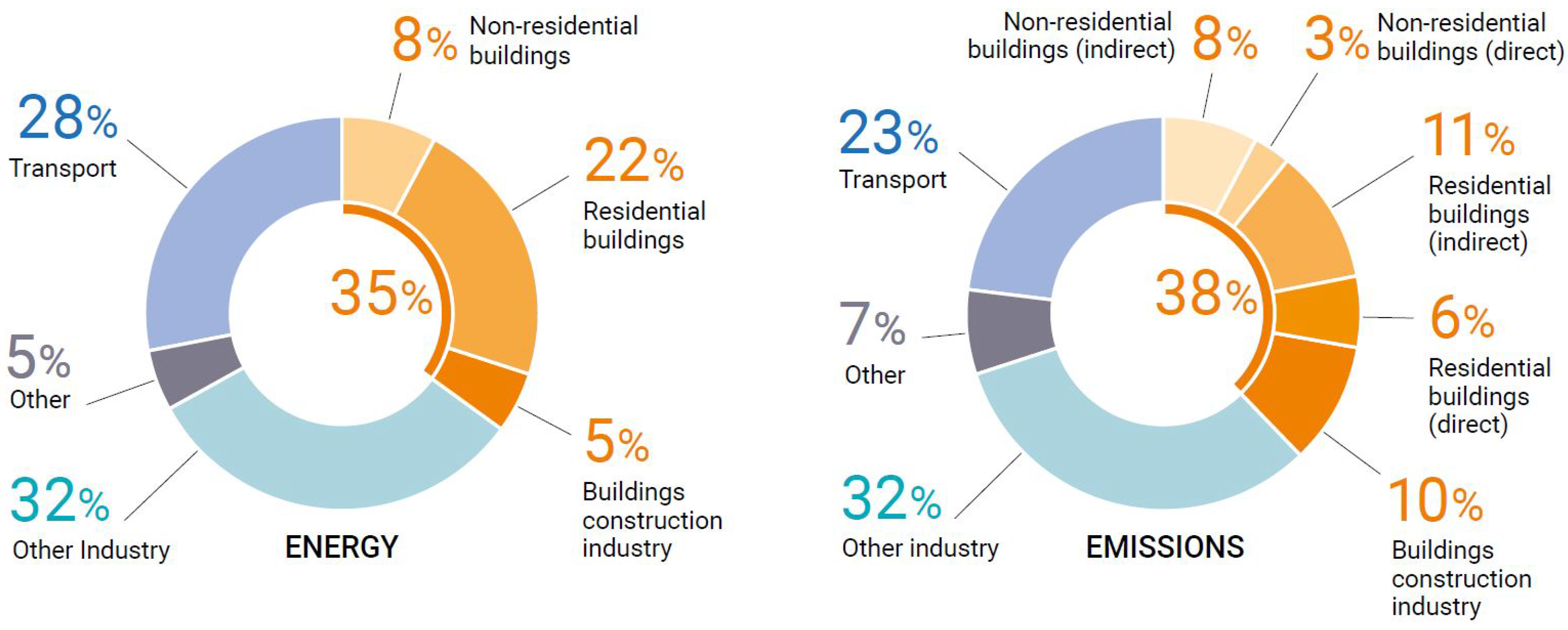
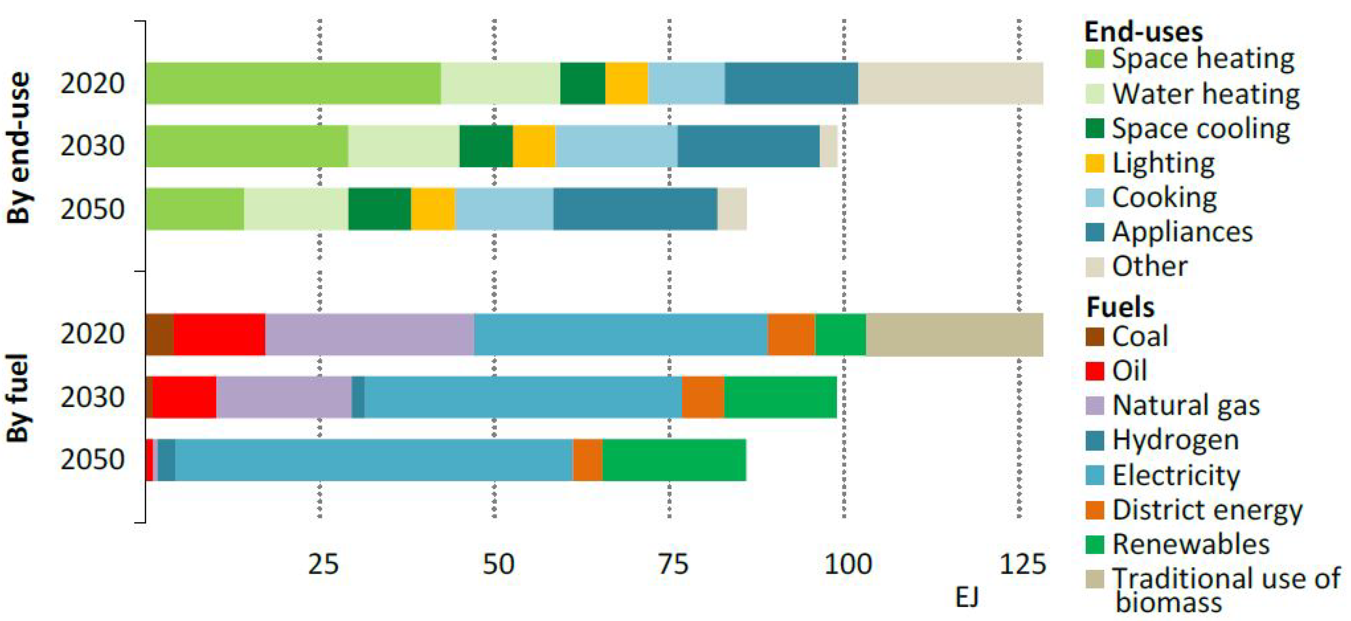
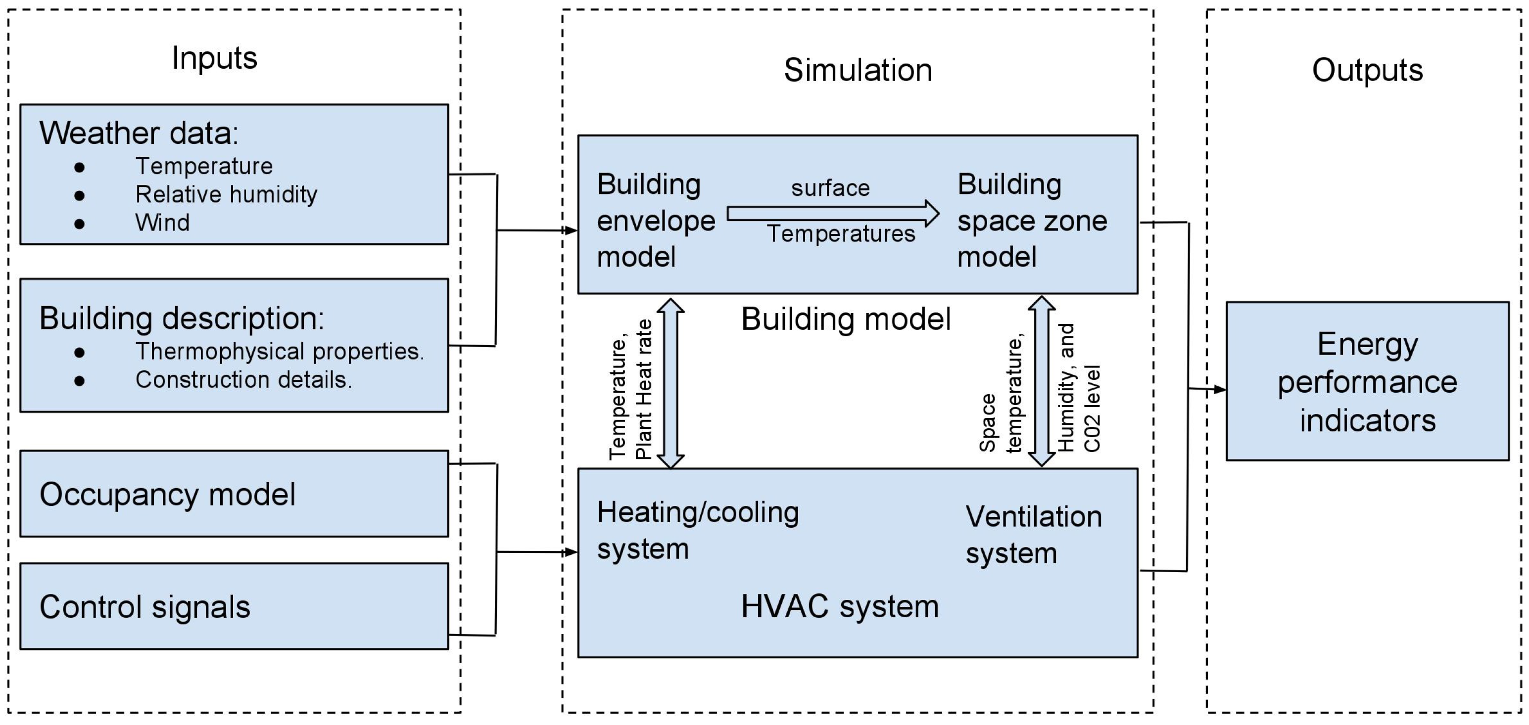
:1. Introduction
Building Thermal Models
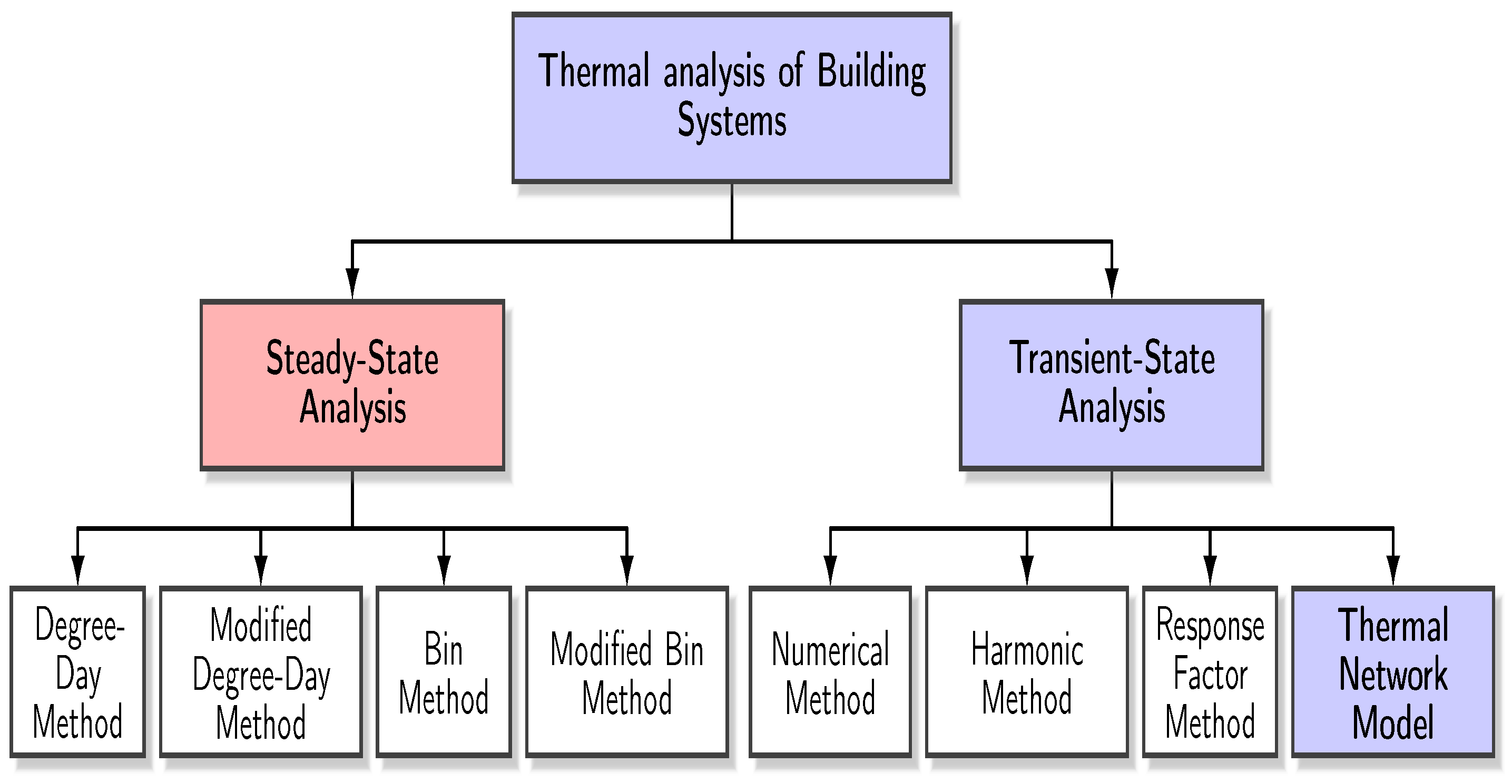
- Steady-state models
- Dynamic/Transient models
- Analytical (white-box) models: are a physical modeling approach relying on thermodynamic and/or mathematical equations, and engineering methods for energy modeling. Some examples are the building energy analysis simulation software programs such as EnergyPlus [29], the Transient System Simulation Tool (TRNSYS) [30], eQuest, etc. Data for all the thermo-physical characteristics are required to develop white-box models. The complexity of these models increases with an increase in the size of a building, thus resulting in high computational costs. These models are not suitable for controller applications.
- Data-driven (black-box) models: are data-driven building energy models, which are built on the basis of available data [31,32] are often considered easy to model compared to physics-based white-box models. Black-box model examples are Artificial Neural Networks (ANNs) [33], Support Vector Machines (SVM) [34], Genetic Algorithms (GAs) [35], Reinforcement Learning models (RL), deep machine learning models [36], etc. Aside from their ease of application, black-box models, require large amounts of input data to train the model. This data may not be available in buildings where sensors are not installed, thereby limiting their application to the few buildings with installed sensors.
- Hybrid (gray-box) models: to overcome white-box and black-box model drawbacks, hybrid (gray-box) models were introduced [37]. Gray-box models are a combination of physics-based models (white-box models) and statistical methods (black-box models). Gray-box modeling is found to be the most robust and accurate method for modeling building systems and improving building performance [38]. These models were mainly developed using the lumped-capacitance method, which includes a network of thermal resistors and capacitors (called a thermal-network model).
2. Thermal-Network Models
- 1.
- Model for a building envelope (walls, floors, roofs, etc.).
- 2.
- Model for space-zone and its thermal interactions with the envelope.
- 3.
- Model for a complete zone.
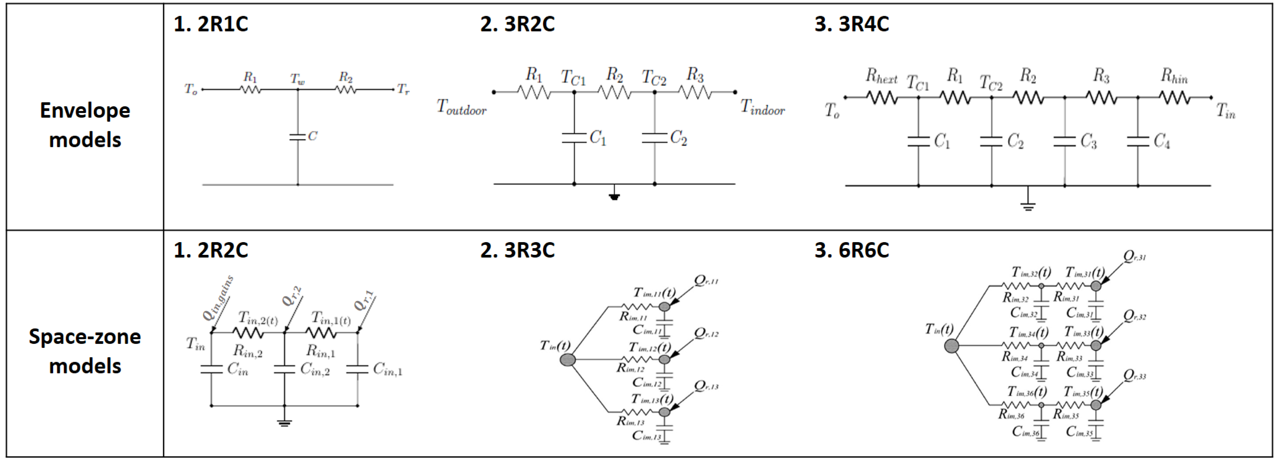
2.1. Building Envelope Models
2.2. Models for Space-Zones and Their Thermal Interactions with Envelopes
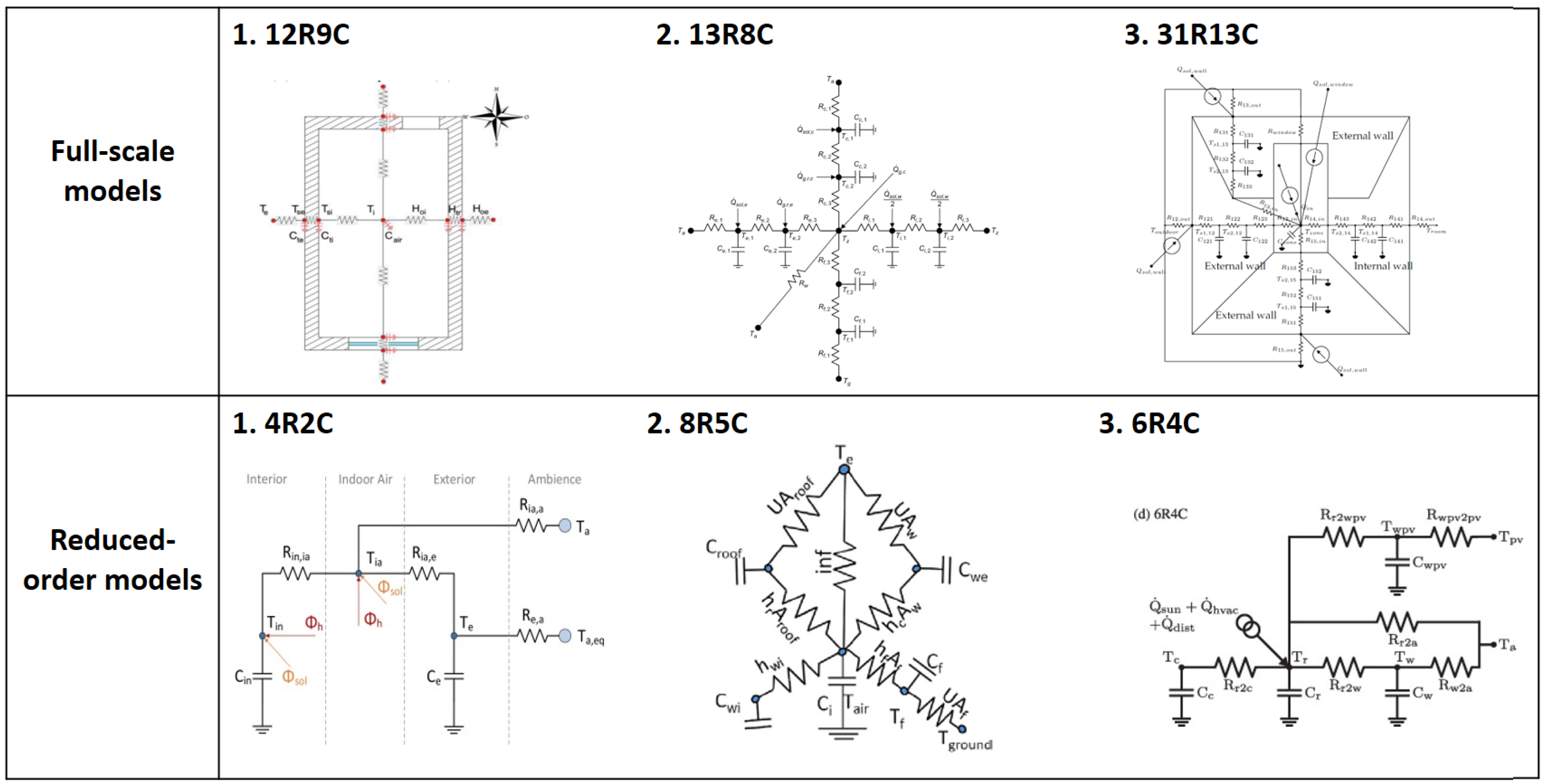
2.3. Models for a Complete-Zone Full-Scale Model
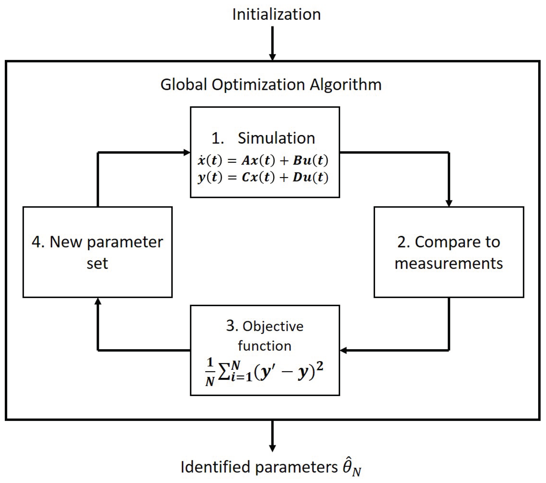
3. Parametric Identification
- Forward/direct methods
- Inverse methods
- Hybrid methods
3.1. Forward/Direct Methods
3.2. Inverse Models
- Parameter estimation: Inverse modeling is used to determine the parameters, such as resistor or capacitor values in the thermal-network model. These parameters will have some physical meaning and boundaries during the optimization.
- System identification: The inverse modeling is applied to identify complete systems with all parameters that may or may not have any physical meaning. These models use patterns to predict the system’s dynamics.
- Deterministic models
- Stochastic time series models
- Black-box models

| Reference | Building Type | Thermal-Network Model | Optimization Method/Algorithm | Simulation Tool | Simulation Period | Performance Metrics | Contributions | Limitations |
|---|---|---|---|---|---|---|---|---|
| [60] | University | Multi-zone | Maximum likelihood estimator | MATLAB | 48 h | Sum squared error (SSE) | Convective heat transfer between zones is considered and parameters are estimated for the same zone | Zone temperatures are maintained at a constant value (closed-loop data), this is likely to lead to grossly inaccurate parameter estimation |
| [147] | Residential | 5R2C | Least squares identification | MATLAB | 120 days | fit | The models for input systems are modeled and linearised to obtain simple models | Physical interpretation of obtained parameter values are not studied. Furthermore, the boundaries of parameter values are not clearly stated. |
| [105] | Monumental | Multiple configurations | GA, pattern search, fmincon | MATLAB | 1 year | fit, mean squared error (MSE), mean absolute error (MAE) | Simplified hygrothermal model is developed with multiple parametric optimization methods. Indoor temperature and RH are predicted for free floating monumental building with higher accuracy | Sensitivity analysis is not conducted. The computation time complexity for optimization process is high, as is the difference between each optimization algorithm output parameter. |
| [95] | Office | 6R2C | Interior point algorithm | Training : 1,2,3 weeks, Test : 3 weeks | fit, RMSE, energy relative error (ERE) | Multiple RC models are compared. Sensitivity analyses of parameters are presented. | Robustness of the proposed model should be validated for long-term predictions. | |
| [89] | Lodging | 1R1C | Nelder–Mead simplex algorithm | Parametric estimation : 12 days, model simulation : 2 and 4 days | RMS and MAE | Multiple RC models are compared. On-line estimation of occupancy heat gains is estimated and included in the model. | The model should be validated for long-term predictions. Physical interpretations of parameters are not included. | |
| [123] | Residential | Envelope model - 2R1C | Bayesian analysis | CERN MINUIT [148] | 14 days | Combining physical and Bayesian analyses lead to significantly reduced measurement periods required to estimate U- and R-values compared to conventional steady-state methods. | Lower order RC model is not suitable for the high thermal mass walls. Robustness of the methodology should be verified for different materials. | |
| [111] | Office | 3R3C | least squares algorithm | MATLAB | 3, 7, 21, and 42 days | RMSE | Gaussian process (GP) is developed to represent building dynamics. The prediction errors for occupied period are 27% lower than gray-box models. | Long-term simulation is not studied. Dynamic occupancy, and other heat inputs are not fully taken into account. |
| [149] | Office | Envelope model - 2R1C and 3R2C | Maximum a posteriori (MAP) and bayesian analysis | SciPy [150] | 3 days | fit | R and C values are estimated for building envelopes based on in-situ measurements. The positioning of R and C parameters are optimally positioned in 3R2C model | The methodology to chose parameter boundary values is not clearly presented. |
| [142] | Office | 4R2C | System identification toolbox | MATLAB | 1 day | fit | EMSs are developed based on mixed integer linear programming (MILP) to optimize the bi-directional energy flow while managing thermal comfort. | Selection of model structure is not discussed. Physical interpretation of each parameter is ignored. |
| [151] | Office | Multi-zone | GA and Prediction Error Method (PEM) | MATLAB | 17 days | fit and RMSE | Model reduction by removing non-identifiable parameters is presented. This also reduced the model uncertainty significantly. | Zone temperatures are maintained at a constant value (closed-loop data), this likely to lead to grossly inaccurate parameter estimation |
| [152] | University | 3R2C | Profile likelihood method [153,154] | RMSE | UKF and EnKF have been compared for the purpose of estimating residuals and covariance for evaluation of the likelihood function. | Closed-loop data is used for validation, this is likely to lead to grossly inaccurate parameter estimations |
3.3. Hybrid Models
4. Conclusions and Perspectives
- The models that are developed for envelopes are not generic and multiple configurations are presented. Therefore, research on development of a generic model to represent thermal dynamics through building envelopes (considering multiple types of thermal mass walls) is essential.
- As noted by authors, full-scale models are accurate but become complex when applied for multi-zone buildings. More research is needed on model reduction and calibrations techniques.
- In most studies, there is still a lack of analysis on the models’ suitability for seasonal variations, dynamic occupancy, and short and long-term simulations.
- Analysis of proper input selection and consideration of all influential inputs is still required.
- Comprehensive analysis on the development of hygric models (including latent heat and mass transfer dynamics) is essential. These models can be used to simulate indoor thermal conditions with greater accuracy.
- Most parametric and system identification studies lack a thorough explanation of model structure selection, physical interpretation of identified parameters, and boundary values selection during the optimization process.
- Uncertainty analysis of measured and simulated data is still poorly studied in the literature and has not been considered in most studies.
Author Contributions
Funding
Conflicts of Interest
Abbreviations
| ANN | Artificial neural networks |
| ARMAX | Auto-regressive moving average with external inputs |
| ARX | Auto-regressive with external inputs |
| BEMS | Building energy management system |
| BIM | Building information modeling |
| BJ | Box-jenkins |
| BSAS | Beetle swarm antenna search |
| Bi | Biot number |
| CSTM | Continuous time stochastic modeling) |
| CTF | Conduction transfer function |
| DLM | Dominant layer model |
| EKF | Extended Kalman filter |
| EMS | Energy management systems |
| ERE | Energy relative error |
| EU | European union |
| GA | Genetic algorithms |
| GHG | Greenhouse gases |
| GP | Gaussian process |
| HVAC | Heating, ventilation, and air-conditioning systems |
| IEA | International energy agency |
| MAE | Mean absolute error |
| MAP | Maximum a posteriori |
| MILP | Mixed integer linear programming |
| MPC | Model predictive controller |
| MSE | Mean squared error |
| NZE | Net zero energy |
| OE | Output error |
| PCM | Phase-change materials |
| PEM | Prediction error method |
| PRBS | Pseudo-random binary sequence signal |
| PSO | Particle swarm optimization |
| RL | Reinforcement learning |
| RMSE | Root mean square error |
| SSE | Sum squared-error |
| SVM | Support vector machine |
| TRNSYS | Transient system simulation tool |
| UHI | Urban heat intensity |
| UKF | unscented Kalman filtering |
References
- Energy Technology Perspectives 2020; Technical Report; IEA: Paris, France, 2020.
- World Energy Balances 2020; Technical Report; IEA: Paris, France, 2020.
- 2020 Global Status Report for Buildings and Construction: Towards a Zero-Emission, Efficient and Resilient Buildings and Construction Sector; Technical Report; United Nations Environment Programme: Nairobi, Kenya, 2020.
- Layke, J.; Mackres, E. Building Efficiency Finally Gets its Day in the Sun at COP 21; World Resources Institute: Washington, DC, USA, 2015. [Google Scholar]
- Global ABC Roadmap for Buildings and Construction; Technical Report; Global Alliance for Buildings and Construction (GlobalABC): Paris, France, 2020.
- Rocha, P.; Siddiqui, A.; Stadler, M. Improving energy efficiency via smart building energy management systems: A comparison with policy measures. Energy Build. 2015, 88, 203–213. [Google Scholar] [CrossRef] [Green Version]
- Net Zero by 2050—A Roadmap for the Global Energy Sector; Technical report; IEA Publications, International Energy Agency: Paris, France, 2021.
- González, A.B.R.; Díaz, J.J.V.; Caamaño, A.J.; Wilby, M.R. Towards a universal energy efficiency index for buildings. Energy Build. 2011, 43, 980–987. [Google Scholar] [CrossRef]
- Song, M.; Niu, F.; Mao, N.; Hu, Y.; Deng, S. Review on building energy performance improvement using phase change materials. Energy Build. 2018, 158, 776–793. [Google Scholar] [CrossRef]
- Sadineni, S.B.; Madala, S.; Boehm, R.F. Passive building energy savings: A review of building envelope components. Renew. Sustain. Energy Rev. 2011, 15, 3617–3631. [Google Scholar] [CrossRef]
- Gaur, A.S.; Fitiwi, D.Z.; Curtis, J. Heat pumps and our low-carbon future: A comprehensive review. Energy Res. Soc. Sci. 2021, 71, 101764. [Google Scholar] [CrossRef]
- Hannan, M.A.; Faisal, M.; Ker, P.J.; Mun, L.H.; Parvin, K.; Mahlia, T.M.I.; Blaabjerg, F. A Review of Internet of Energy Based Building Energy Management Systems: Issues and Recommendations. IEEE Access 2018, 6, 38997–39014. [Google Scholar] [CrossRef]
- Kanthila, C.; Boodi, A.; Beddiar, K.; Amirat, Y.; Benbouzid, M. Building Occupancy Behavior and Prediction Methods: A Critical Review and Challenging Locks. IEEE Access 2021, 9, 79353–79372. [Google Scholar] [CrossRef]
- Boodi, A.; Beddiar, K.; Benamour, M.; Amirat, Y.; Benbouzid, M. Intelligent systems for building energy and occupant comfort optimization: A state of the art review and recommendations. Energies 2018, 11, 2604. [Google Scholar] [CrossRef] [Green Version]
- ASHRAE. 2017 ASHRAE Handbook–Fundamentals (SI Edition); American Society of Heating, Refrigerating and Air-Conditioning Engineers: Atlanta, GA, USA, 2017. [Google Scholar]
- Wen, J.T.; Mishra, S. Intelligent Building Control Systems; Springer: Cham, Switzerland, 2018. [Google Scholar]
- Underwood, C.P.; Yik, F.W. Modelling Methods for Energy in Buildings; John Wiley & Sons: Hoboken, NJ, USA, 2008. [Google Scholar] [CrossRef]
- Papantoniou, S.; Kolokotsa, D.; Kalaitzakis, K. Building optimization and control algorithms implemented in existing BEMS using a web based energy management and control system. Energy Build. 2015, 98, 45–55. [Google Scholar] [CrossRef]
- Lee, D.; Cheng, C.C. Energy savings by energy management systems: A review. Renew. Sustain. Energy Rev. 2016, 56, 760–777. [Google Scholar] [CrossRef]
- Manic, M.; Wijayasekara, D.; Amarasinghe, K.; Rodriguez-Andina, J.J. Building energy management systems: The age of intelligent and adaptive buildings. IEEE Ind. Electron. Mag. 2016, 10, 25–39. [Google Scholar] [CrossRef]
- Amasyali, K.; El-Gohary, N.M. A review of data-driven building energy consumption prediction studies. Renew. Sustain. Energy Rev. 2018, 81, 1192–1205. [Google Scholar] [CrossRef]
- Wang, Z.; Srinivasan, R.S. A review of artificial intelligence based building energy use prediction: Contrasting the capabilities of single and ensemble prediction models. Renew. Sustain. Energy Rev. 2017, 75, 796–808. [Google Scholar] [CrossRef]
- Široký, J.; Oldewurtel, F.; Cigler, J.; Prívara, S. Experimental analysis of model predictive control for an energy efficient building heating system. Appl. Energy 2011, 88, 3079–3087. [Google Scholar] [CrossRef]
- Avci, M.; Erkoc, M.; Rahmani, A.; Asfour, S. Model predictive HVAC load control in buildings using real-time electricity pricing. Energy Build. 2013, 60, 199–209. [Google Scholar] [CrossRef]
- Prívara, S.; Široký, J.; Ferkl, L.; Cigler, J. Model predictive control of a building heating system: The first experience. Energy Build. 2011, 43, 564–572. [Google Scholar] [CrossRef]
- Dobbs, J.R.; Hencey, B.M. Model predictive HVAC control with online occupancy model. Energy Build. 2014, 82, 675–684. [Google Scholar] [CrossRef] [Green Version]
- Boodi, A.; Beddiar, K.; Amirat, Y.; Benbouzid, M. Simplified Building Thermal Model Development and Parameters Evaluation Using a Stochastic Approach. Energies 2020, 13, 2899. [Google Scholar] [CrossRef]
- Al-Homoud, M.S. Computer-aided building energy analysis techniques. Build. Environ. 2001, 36, 421–433. [Google Scholar] [CrossRef]
- Crawley, D.B.; Lawrie, L.K.; Winkelmann, F.C.; Buhl, W.F.; Huang, Y.J.; Pedersen, C.O.; Strand, R.K.; Liesen, R.J.; Fisher, D.E.; Witte, M.J. EnergyPlus: Creating a new-generation building energy simulation program. Energy Build. 2001, 33, 319–331. [Google Scholar] [CrossRef]
- University of Wisconsin–Madison. Solar Energy Laboratory. TRNSYS, a Transient Simulation Program; The Laboratory: Madison, WI, USA, 1975. [Google Scholar]
- Panchabikesan, K.; Haghighat, F.; Mankibi, M.E. Data driven occupancy information for energy simulation and energy use assessment in residential buildings. Energy 2021, 218, 119539. [Google Scholar] [CrossRef]
- Ahmad, T.; Chen, H.; Guo, Y.; Wang, J. A comprehensive overview on the data driven and large scale based approaches for forecasting of building energy demand: A review. Energy Build. 2018, 165, 301–320. [Google Scholar] [CrossRef]
- Schalkoff, R.J. Artificial Neural Networks; McGraw-Hill Higher Education: New York, NY, USA, 1997. [Google Scholar]
- Hearst, M.A.; Dumais, S.T.; Osuna, E.; Platt, J.; Scholkopf, B. Support vector machines. IEEE Intell. Syst. Their Appl. 1998, 13, 18–28. [Google Scholar] [CrossRef] [Green Version]
- Whitley, D. A genetic algorithm tutorial. Stat. Comput. 1994, 4, 65–85. [Google Scholar] [CrossRef]
- Goodfellow, I.; Bengio, Y.; Courville, A. Deep Learning; MIT Press: Cambridge, MA, USA, 2016. [Google Scholar]
- Oussar, Y.; Dreyfus, G. How to be a gray box: Dynamic semi-physical modeling. Neural Netw. 2001, 14, 1161–1172. [Google Scholar] [CrossRef]
- Braun, J.E.; Chaturvedi, N. An Inverse Gray-Box Model for Transient Building Load Prediction. HVAC&R Res. 2002, 8, 73–99. [Google Scholar]
- Evins, R. A review of computational optimisation methods applied to sustainable building design. Renew. Sustain. Energy Rev. 2013, 22, 230–245. [Google Scholar] [CrossRef]
- Al-Ghaili, A.M.; Kasim, H.; Al-Hada, N.M.; Jørgensen, B.N.; Othman, M.; Jihua, W. Energy Management Systems and Strategies in Buildings Sector: A Scoping Review. IEEE Access 2021, 9, 63790–63813. [Google Scholar] [CrossRef]
- Sbiti, M.; Beddiar, K.; Beladjine, D.; Perrault, R.; Mazari, B. Toward BIM and LPS Data Integration for Lean Site Project Management: A State-of-the-Art Review and Recommendations. Buildings 2021, 11, 196. [Google Scholar] [CrossRef]
- Mohammed, B.H.; Safie, N.; Sallehuddin, H.; Hussain, A.H.B. Building Information Modelling (BIM) and the Internet-of-Things (IoT): A Systematic Mapping Study. IEEE Access 2020, 8, 155171–155183. [Google Scholar] [CrossRef]
- Zalba, B.; Marın, J.M.; Cabeza, L.F.; Mehling, H. Review on thermal energy storage with phase change: Materials, heat transfer analysis and applications. Appl. Therm. Eng. 2003, 23, 251–283. [Google Scholar] [CrossRef]
- Webb, A.L. Energy retrofits in historic and traditional buildings: A review of problems and methods. Renew. Sustain. Energy Rev. 2017, 77, 748–759. [Google Scholar] [CrossRef]
- D’Oca, S.; Hong, T.; Langevin, J. The human dimensions of energy use in buildings: A review. Renew. Sustain. Energy Rev. 2018, 81, 731–742. [Google Scholar] [CrossRef] [Green Version]
- Al-Ghaili, A.M.; Kasim, H.; Al-Hada, N.M.; Othman, M.; Saleh, M.A. A Review: Buildings Energy Savings-Lighting Systems Performance. IEEE Access 2020, 8, 76108–76119. [Google Scholar] [CrossRef]
- Li, X.; Wen, J. Review of building energy modeling for control and operation. Renew. Sustain. Energy Rev. 2014, 37, 517–537. [Google Scholar] [CrossRef]
- Dounis, A.I.; Caraiscos, C. Advanced control systems engineering for energy and comfort management in a building environment—A review. Renew. Sustain. Energy Rev. 2009, 13, 1246–1261. [Google Scholar] [CrossRef]
- Parvin, K.; Lipu, M.H.; Hannan, M.A.; Abdullah, M.A.; Jern, K.P.; Begum, R.A.; Mansur, M.; Muttaqi, K.M.; Mahlia, T.I.; Dong, Z.Y. Intelligent Controllers and Optimization Algorithms for Building Energy Management Towards Achieving Sustainable Development: Challenges and Prospects. IEEE Access 2021, 9, 41577–41602. [Google Scholar] [CrossRef]
- Wei, Y.; Zhang, X.; Shi, Y.; Xia, L.; Pan, S.; Wu, J.; Han, M.; Zhao, X. A review of data-driven approaches for prediction and classification of building energy consumption. Renew. Sustain. Energy Rev. 2018, 82, 1027–1047. [Google Scholar] [CrossRef]
- Pohekar, S.D.; Ramachandran, M. Application of multi-criteria decision making to sustainable energy planning—A review. Renew. Sustain. Energy Rev. 2004, 8, 365–381. [Google Scholar] [CrossRef]
- Schmidt, M.; Åhlund, C. Smart buildings as Cyber-Physical Systems: Data-driven predictive control strategies for energy efficiency. Renew. Sustain. Energy Rev. 2018, 90, 742–756. [Google Scholar] [CrossRef] [Green Version]
- Mirakhorli, A.; Dong, B. Occupancy behavior based model predictive control for building indoor climate—A critical review. Energy Build. 2016, 129, 499–513. [Google Scholar] [CrossRef]
- Serale, G.; Fiorentini, M.; Capozzoli, A.; Bernardini, D.; Bemporad, A. Model Predictive Control (MPC) for Enhancing Building and HVAC System Energy Efficiency: Problem Formulation, Applications and Opportunities. Energies 2018, 11, 631. [Google Scholar] [CrossRef] [Green Version]
- Rupp, R.F.; Vásquez, N.G.; Lamberts, R. A review of human thermal comfort in the built environment. Energy Build. 2015, 105, 178–205. [Google Scholar] [CrossRef]
- Kanthila, C.; Boodi, A.; Beddiar, K.; Amirat, Y.; Benbouzid, M. Markov Chain-based Algorithms for Building Occupancy Modeling: A Review. In Proceedings of the 2021 3rd International Conference on Smart Power & Internet Energy Systems (SPIES), Shanghai, China, 25–28 September 2021; pp. 438–443. [Google Scholar]
- Kramer, R.; van Schijndel, J.; Schellen, H. Simplified thermal and hygric building models: A literature review. Front. Archit. Res. 2012, 1, 318–325. [Google Scholar] [CrossRef] [Green Version]
- Bagheri, A.; Feldheim, V.; Ioakimidis, C. On the Evolution and Application of the Thermal Network Method for Energy Assessments in Buildings. Energies 2018, 11, 890. [Google Scholar] [CrossRef] [Green Version]
- Robertson, A.F.; Gross, D. An Electrical-Analog Method for Transient Heat-Flow. J. Res. Natl. Bur. Stand. 1958, 61, 2892. [Google Scholar] [CrossRef]
- Goyal, S.; Liao, C.; Barooah, P. Identification of multi-zone building thermal interaction model from data. In Proceedings of the 2011 50th IEEE Conference on Decision and Control and European Control Conference, Orlando, FL, USA, 12–15 December 2011; pp. 181–186. [Google Scholar] [CrossRef]
- Gouda, M.; Danaher, S.; Underwood, C. Building thermal model reduction using nonlinear constrained optimization. Build. Environ. 2002, 37, 1255–1265. [Google Scholar] [CrossRef]
- Kircher, K.J.; Max Zhang, K. On the lumped capacitance approximation accuracy in RC network building models. Energy Build. 2015, 108, 454–462. [Google Scholar] [CrossRef] [Green Version]
- Bueno, B.; Norford, L.; Pigeon, G.; Britter, R. A resistance-capacitance network model for the analysis of the interactions between the energy performance of buildings and the urban climate. Build. Environ. 2012, 54, 116–125. [Google Scholar] [CrossRef]
- Xu, X.; Wang, S. A simplified dynamic model for existing buildings using CTF and thermal-network models. Int. J. Therm. Sci. 2008, 47, 1249–1262. [Google Scholar] [CrossRef]
- Boodi, A. On Energy-Efficient Buildings: Hybrid Dynamic Modeling for Analysis and Control. Ph.D. Thesis, Université de Bretagne Occidentale, Brest, France, 2021. [Google Scholar]
- Lorenz, F.; Masy, G. Méthode d’évaluation de l’économie d’énergie apportée par l’intermittence de chauffage dans les bâtiments. In Traitement par Differences Finies d’un Model a deux Constantes de Temps; Report No. GM820130-01; Faculte des Sciences Appliquees, University de Liege: Liege, Belgium, 1982. [Google Scholar]
- Fraisse, G.; Viardot, C.; Lafabrie, O.; Achard, G. Development of a simpli®ed and accurate building model based on electrical analogy. Energy Build. 2002, 34, 1017–1031. [Google Scholar] [CrossRef]
- Wang, S.; Xu, X. Simplified building model for transient thermal performance estimation using GA-based parameter identification. Int. J. Therm. Sci. 2006, 45, 419–432. [Google Scholar] [CrossRef]
- Ji, Y.; Xu, P.; Duan, P.; Lu, X. Estimating hourly cooling load in commercial buildings using a thermal-network model and electricity submetering data. Appl. Energy 2016, 169, 309–323. [Google Scholar] [CrossRef]
- Hassid, S. A linear model for passive solar calculations: Evaluation of performance. Build. Environ. 1985, 20, 53–59. [Google Scholar] [CrossRef]
- Tindale, A. Third-order lumped-parameter simulation method. Build. Serv. Eng. Res. Technol. 1993, 14, 87–97. [Google Scholar] [CrossRef]
- Lombard, C.; Mathews, E. A two-port envelope model for building heat transfer. Build. Environ. 1998, 34, 19–30. [Google Scholar] [CrossRef]
- Gouda, M.; Danaher, S.; Underwood, C. Low-order model for the simulation of a building and its heating system. Build. Serv. Eng. Res. Technol. 2000, 21, 199–208. [Google Scholar] [CrossRef]
- Underwood, C.P. An improved lumped parameter method for building thermal modelling. Energy Build. 2014, 79, 191–201. [Google Scholar] [CrossRef] [Green Version]
- Lombard, C.; Mathews, E. Efficient, steady state solution of a time variable RC network, for building thermal analysis. Build. Environ. 1992, 27, 279–287. [Google Scholar] [CrossRef]
- Madsen, H.; Holst, J. Estimation of continuous-time models for the heat dynamics of a building. Energy Build. 1995, 22, 67–79. [Google Scholar] [CrossRef]
- Hudson, G.; Underwood, C.P. A simple building modelling procedure for MATLAB/SIMULINK. In Proceedings of the International Building Performance and Simulation Conference, Kyoto, Japan, 13–15 September 1999; Citeseer: Pittsburgh, PA, USA, 1999; Volume 2, pp. 777–783. [Google Scholar]
- Wang, S. Dynamic simulation of building VAV air-conditioning system and evaluation of EMCS on-line control strategies. Build. Environ. 1999, 34, 681–705. [Google Scholar] [CrossRef]
- Tashtoush, B.; Molhim, M.; Al-Rousan, M. Dynamic model of an HVAC system for control analysis. Energy 2005, 30, 1729–1745. [Google Scholar] [CrossRef]
- Harish, V.; Kumar, A. Reduced order modeling and parameter identification of a building energy system model through an optimization routine. Appl. Energy 2016, 162, 1010–1023. [Google Scholar] [CrossRef]
- Freier, J.; Ceccolini, C.; Arnold, M.; Hesselbach, J. A Lumped-Capacitance Model for the Assessment of Energy Flexibility in different Building Typologies. In Proceedings of the 2020 55th International Universities Power Engineering Conference (UPEC), Turin, Italy, 1–4 September 2020; pp. 1–6. [Google Scholar] [CrossRef]
- Liao, Z.; Dexter, A. A simplified physical model for estimating the average air temperature in multi-zone heating systems. Build. Environ. 2004, 39, 1013–1022. [Google Scholar] [CrossRef]
- Wang, S.; Xu, X. Parameter estimation of internal thermal mass of building dynamic models using genetic algorithm. Energy Convers. Manag. 2006, 47, 1927–1941. [Google Scholar] [CrossRef]
- Park, H.; Ruellan, M.; Bennacer, R.; Monmasson, E. Thermal network of coupled building and electrical appliances. Mech. Ind. 2016, 17, 102. [Google Scholar] [CrossRef]
- Park, H.; Ruellan, M.; Bouvet, A.; Monmasson, E.; Bennacer, R. Thermal parameter identification of simplified building model with electric appliance. In Proceedings of the 11th International Conference on Electrical Power Quality and Utilisation, Lisbon, Portugal, 17–19 October 2011; pp. 1–6. [Google Scholar] [CrossRef]
- Harb, H.; Boyanov, N.; Hernandez, L.; Streblow, R.; Müller, D. Development and validation of grey-box models for forecasting the thermal response of occupied buildings. Energy Build. 2016, 117, 199–207. [Google Scholar] [CrossRef]
- Danza, L.; Belussi, L.; Meroni, I.; Salamone, F.; Floreani, F.; Piccinini, A.; Dabusti, A. A Simplified Thermal Model to Control the Energy Fluxes and to Improve the Performance of Buildings. Energy Procedia 2016, 101, 97–104. [Google Scholar] [CrossRef]
- Reynders, G.; Diriken, J.; Saelens, D. Quality of grey-box models and identified parameters as function of the accuracy of input and observation signals. Energy Build. 2014, 82, 263–274. [Google Scholar] [CrossRef]
- Fux, S.F.; Ashouri, A.; Benz, M.J.; Guzzella, L. EKF based self-adaptive thermal model for a passive house. Energy Build. 2014, 68, 811–817. [Google Scholar] [CrossRef]
- Bacher, P.; Madsen, H. Identifying suitable models for the heat dynamics of buildings. Energy Build. 2011, 43, 1511–1522. [Google Scholar] [CrossRef] [Green Version]
- Juhl, R.; Møller, J.K.; Madsen, H. Ctsmr—Continuous time stochastic modeling in R. arXiv 2016, arXiv:1606.00242. [Google Scholar]
- Palomo Del Barrio, E.; Lefebvre, G.; Behar, P.; Bailly, N. Using model size reduction techniques for thermal control applications in buildings. Energy Build. 2000, 33, 1–14. [Google Scholar] [CrossRef]
- Mejri, O.; Palomo Del Barrio, E.; Ghrab-Morcos, N. Energy performance assessment of occupied buildings using model identification techniques. Energy Build. 2011, 43, 285–299. [Google Scholar] [CrossRef]
- Massano, M.; Macii, E.; Patti, E.; Acquaviva, A.; Bottaccioli, L. A Grey-box Model Based on Unscented Kalman Filter to Estimate Thermal Dynamics in Buildings. In Proceedings of the 2019 IEEE International Conference on Environment and Electrical Engineering and 2019 IEEE Industrial and Commercial Power Systems Europe (EEEIC/I CPS Europe), Genova, Italy, 11–14 June 2019; pp. 1–6. [Google Scholar] [CrossRef]
- Berthou, T.; Stabat, P.; Salvazet, R.; Marchio, D. Development and validation of a gray box model to predict thermal behavior of occupied office buildings. Energy Build. 2014, 74, 91–100. [Google Scholar] [CrossRef]
- VDI 6007-Calculation of the Transient Thermal Behavior of Rooms and Buildings, VDI. 2016. Available online: https://www.vdi.de/ (accessed on 20 November 2021).
- Comité Europeo de Normalización. EN ISO 13790: Energy Performance of Buildings: Calculation of Energy Use for Space Heating and Cooling (ISO 13790: 2008); CEN: Brussels, Belgium, 2008. [Google Scholar]
- Michalak, P. A thermal-network model for the dynamic simulation of the energy performance of buildings with the time varying ventilation flow. Energy Build. 2019, 202, 109337. [Google Scholar] [CrossRef]
- European Standards, DIN EN 12831-1, Energy Performance of Buildings- Method for Calculation of the Design Heat Load-Part 1: Space Heating Load, Module M3-3. 2017. Available online: https://www.en-standard.eu/ (accessed on 4 December 2021).
- DIN, V. 18599, Energy Efficiency of Buildings–Calculation of the Net, Final and Primary Energy Demand for Heating, Cooling, Ventilation, Domestic Hot Water and Lighting; Deutsche Norm; Deutsches Institut für Normung: Berlin, Germany, 2007. [Google Scholar]
- Comité Européen de Normalisation. Water Based Surface Embedded Heating and Cooling Systems—Part 2: Floor Heating: Prove Methods for the Determination of the Thermal Output Using Calculation and Test Methods; Standard No. EN1264-2; CEN: Brussels, Belgium, 2008. [Google Scholar]
- Recknagel, H. Taschenbuch für Heizung und Klimatechnik: Einschlieąlich Warmwasser-und Kältetechnik: Mit über 2100 Abbildungen und über 350 Tafeln sowie 4 Einschlagtafeln; Oldenbourg Industrieverlag: Munich, Germany, 2011. [Google Scholar]
- Fonti, A.; Comodi, G.; Pizzuti, S.; Arteconi, A.; Helsen, L. Low Order Grey-box Models for Short-term Thermal Behavior Prediction in Buildings. Energy Procedia 2017, 105, 2107–2112. [Google Scholar] [CrossRef]
- MATLAB. Version 7.10.0 (R2010a); The MathWorks Inc.: Natick, MA, USA, 2010. [Google Scholar]
- Kramer, R.; van Schijndel, J.; Schellen, H. Inverse modeling of simplified hygrothermal building models to predict and characterize indoor climates. Build. Environ. 2013, 68, 87–99. [Google Scholar] [CrossRef]
- Sayadi, S.; Tsatsaronis, G.; Morosuk, T. Reducing the energy consumption of HVAC systems in buildings by using model predictive control. In Proceedings of the CLIMA, Aalborg, Denmark, 22–26 May 2016. [Google Scholar]
- Mahendra, S.; Stephane, P.; Frederic, W. Modeling for reactive building energy management. Energy Procedia 2015, 83, 207–215. [Google Scholar] [CrossRef] [Green Version]
- Goyal, S.; Barooah, P. A method for model-reduction of non-linear thermal dynamics of multi-zone buildings. Energy Build. 2012, 47, 332–340. [Google Scholar] [CrossRef]
- Wilson, M.; Luck, R.; Mago, P. A First-Order Study of Reduced Energy Consumption via Increased Thermal Capacitance with Thermal Storage Management in a Micro-Building. Energies 2015, 8, 12266–12282. [Google Scholar] [CrossRef] [Green Version]
- Massa Gray, F.; Schmidt, M. A hybrid approach to thermal building modelling using a combination of Gaussian processes and grey-box models. Energy Build. 2018, 165, 56–63. [Google Scholar] [CrossRef]
- Gray, F.M.; Schmidt, M. Thermal building modelling using Gaussian processes. Energy Build. 2016, 119, 119–128. [Google Scholar] [CrossRef]
- Wang, J.; Chen, H.; Yuan, Y.; Huang, Y. A novel efficient optimization algorithm for parameter estimation of building thermal dynamic models. Build. Environ. 2019, 153, 233–240. [Google Scholar] [CrossRef]
- Yang, S.; Wan, M.P.; Ng, B.F.; Zhang, T.; Babu, S.; Zhang, Z.; Chen, W.; Dubey, S. A state-space thermal model incorporating humidity and thermal comfort for model predictive control in buildings. Energy Build. 2018, 170, 25–39. [Google Scholar] [CrossRef]
- Belic, F.; Hocenski, Z.; Sliskovic, D. Algorithm for defining structure of thermal model of building based on RC analogy. In Proceedings of the 2019 23rd International Conference on System Theory, Control and Computing (ICSTCC), Sinaia, Romania, 9–11 October 2019; pp. 580–585. [Google Scholar] [CrossRef]
- Vivian, J.; Zarrella, A.; Emmi, G.; De Carli, M. An evaluation of the suitability of lumped-capacitance models in calculating energy needs and thermal behaviour of buildings. Energy Build. 2017, 150, 447–465. [Google Scholar] [CrossRef]
- Kämpf, J.H.; Robinson, D. A simplified thermal model to support analysis of urban resource flows. Energy Build. 2007, 39, 445–453. [Google Scholar] [CrossRef]
- Ogunsola, O.T.; Song, L. Application of a simplified thermal-network model for real-time thermal load estimation. Energy Build. 2015, 96, 309–318. [Google Scholar] [CrossRef]
- Gagliano, A.; Patania, F.; Nocera, F.; Signorello, C. Assessment of the dynamic thermal performance of massive buildings. Energy Build. 2014, 72, 361–370. [Google Scholar] [CrossRef]
- Ghiaus, C.; Hazyuk, I. Calculation of optimal thermal load of intermittently heated buildings. Energy Build. 2010, 42, 1248–1258. [Google Scholar] [CrossRef]
- Ramallo-González, A.P.; Eames, M.E.; Coley, D.A. Lumped parameter models for building thermal modelling: An analytic approach to simplifying complex multi-layered constructions. Energy Build. 2013, 60, 174–184. [Google Scholar] [CrossRef] [Green Version]
- Imanishi, T.; Tennekoon, R.; Palensky, P.; Nishi, H. Enhanced building thermal model by using CO2 based occupancy data. In Proceedings of the IECON 2015-41st Annual Conference of the IEEE Industrial Electronics Society, Yokohama, Japan, 9–12 November 2015; pp. 003116–003121. [Google Scholar] [CrossRef]
- Nielsen, T.R. Simple tool to evaluate energy demand and indoor environment in the early stages of building design. Sol. Energy 2005, 78, 73–83. [Google Scholar] [CrossRef]
- Biddulph, P.; Gori, V.; Elwell, C.A.; Scott, C.; Rye, C.; Lowe, R.; Oreszczyn, T. Inferring the thermal resistance and effective thermal mass of a wall using frequent temperature and heat flux measurements. Energy Build. 2014, 78, 10–16. [Google Scholar] [CrossRef] [Green Version]
- Ogunsola, O.T.; Song, L.; Wang, G. Development and validation of a time-series model for real-time thermal load estimation. Energy Build. 2014, 76, 440–449. [Google Scholar] [CrossRef]
- Afshari, A.; Friedrich, L.A. Inverse modeling of the urban energy system using hourly electricity demand and weather measurements, Part 1: Black-box model. Energy Build. 2017, 157, 126–138. [Google Scholar] [CrossRef]
- Gori, V.; Elwell, C.A. Characterization of the thermal structure of different building constructions using in-situ measurements and Bayesian analysis. Energy Procedia 2017, 132, 537–542. [Google Scholar] [CrossRef]
- Kozadajevs, J.; Broka, Z.; Sauhats, A. Modelling heat demand in buildings with an experimental approach. In Proceedings of the 2017 IEEE International Conference on Environment and Electrical Engineering and 2017 IEEE Industrial and Commercial Power Systems Europe (EEEIC/I CPS Europe), Milan, Italy, 6–9 June 2017; pp. 1–4. [Google Scholar] [CrossRef]
- Virk, G.; Cheung, J.; Loveday, D. Practical stochastic multivariable identification for buildings. Appl. Math. Model. 1995, 19, 621–636. [Google Scholar] [CrossRef]
- Doddi, H.; Talukdar, S.; Deka, D.; Salapaka, M. Data-Driven Identification of a Thermal Network in Multi-Zone Building. In Proceedings of the 2018 IEEE Conference on Decision and Control (CDC), Miami, FL, USA, 17–19 December 2018; pp. 7302–7307. [Google Scholar] [CrossRef] [Green Version]
- Rodríguez Jara, E.Á.; Sánchez de la Flor, F.J.; Álvarez Domínguez, S.; Molina Félix, J.L.; Salmerón Lissén, J.M. A new analytical approach for simplified thermal modelling of buildings: Self-Adjusting RC-network model. Energy Build. 2016, 130, 85–97. [Google Scholar] [CrossRef]
- Rouchier, S. Solving inverse problems in building physics: An overview of guidelines for a careful and optimal use of data. Energy Build. 2018, 166, 178–195. [Google Scholar] [CrossRef]
- Penman, J.M. Second order system identification in the thermal response of a working school. Build. Environ. 1990, 25, 105–110. [Google Scholar] [CrossRef]
- Coley, D.; Penman, J. Second order system identification in the thermal response of real buildings. Paper II: Recursive formulation for on-line building energy management and control. Build. Environ. 1992, 27, 269–277. [Google Scholar] [CrossRef]
- Andersen, K.K.; Madsen, H.; Hansen, L.H. Modelling the heat dynamics of a building using stochastic differential equations. Energy Build. 2000, 31, 13–24. [Google Scholar] [CrossRef] [Green Version]
- Nielsen, H.A.; Madsen, H. Modelling the heat consumption in district heating systems using a grey-box approach. Energy Build. 2006, 38, 63–71. [Google Scholar] [CrossRef] [Green Version]
- Mustafaraj, G.; Chen, J.; Lowry, G. Development of room temperature and relative humidity linear parametric models for an open office using BMS data. Energy Build. 2010, 42, 348–356. [Google Scholar] [CrossRef]
- Peitsman, H.C.; Bakker, V.E. Application of Black-Box Models to HVAC Systems for Fault Detection; Technical Report; American Society of Heating, Refrigerating and Air-Conditioning Engineers: Atlanta, GA, USA, 1996. [Google Scholar]
- Radecki, P.; Hencey, B. Online building thermal parameter estimation via Unscented Kalman Filtering. In Proceedings of the 2012 American Control Conference (ACC), Montreal, QC, Canada, 27–29 June 2012; pp. 3056–3062. [Google Scholar] [CrossRef]
- Rouchier, S.; Jiménez, M.J.; Castaño, S. Sequential Monte Carlo for on-line parameter estimation of a lumped building energy model. Energy Build. 2019, 187, 86–94. [Google Scholar] [CrossRef]
- Lin, Y.; Middelkoop, T.; Barooah, P. Issues in identification of control-oriented thermal models of zones in multi-zone buildings. In Proceedings of the 2012 IEEE 51st IEEE Conference on Decision and Control (CDC), Maui, HI, USA, 10–13 December 2012; pp. 6932–6937. [Google Scholar] [CrossRef]
- Ferracuti, F.; Fonti, A.; Ciabattoni, L.; Pizzuti, S.; Arteconi, A.; Helsen, L.; Comodi, G. Data-driven models for short-term thermal behaviour prediction in real buildings. Appl. Energy 2017, 204, 1375–1387. [Google Scholar] [CrossRef]
- Thomas, D.; Bagheri, A.; Feldheim, V.; Deblecker, O.; Ioakimidis, C.S. Energy and thermal comfort management in a smart building facilitating a microgrid optimization. In Proceedings of the IECON 2017-43rd Annual Conference of the IEEE Industrial Electronics Society, Beijing, China, 29 October–1 November 2017; pp. 3621–3626. [Google Scholar] [CrossRef]
- Afshari, A.; Liu, N. Inverse modeling of the urban energy system using hourly electricity demand and weather measurements, Part 2: Gray-box model. Energy Build. 2017, 157, 139–156. [Google Scholar] [CrossRef]
- Jiménez, M.; Madsen, H.; Andersen, K. Identification of the main thermal characteristics of building components using MATLAB. Build. Environ. 2008, 43, 170–180. [Google Scholar] [CrossRef]
- Rouchier, S.; Rabouille, M.; Oberlé, P. Calibration of simplified building energy models for parameter estimation and forecasting: Stochastic versus deterministic modelling. Build. Environ. 2018, 134, 181–190. [Google Scholar] [CrossRef]
- Brastein, O.; Ghaderi, A.; Pfeiffer, C.; Skeie, N.O. Analysing uncertainty in parameter estimation and prediction for grey-box building thermal behaviour models. Energy Build. 2020, 224, 110236. [Google Scholar] [CrossRef]
- Hazyuk, I.; Ghiaus, C.; Penhouet, D. Optimal temperature control of intermittently heated buildings using Model Predictive Control: Part I–Building modeling. Build. Environ. 2012, 51, 379–387. [Google Scholar] [CrossRef]
- James, F.; Winkler, M. Minuit User’s Guide; CERN: Geneva, Switzerland, 2004; Volume 23. [Google Scholar]
- Gori, V.; Marincioni, V.; Biddulph, P.; Elwell, C.A. Inferring the thermal resistance and effective thermal mass distribution of a wall from in situ measurements to characterise heat transfer at both the interior and exterior surfaces. Energy Build. 2017, 135, 398–409. [Google Scholar] [CrossRef] [Green Version]
- Virtanen, P.; Gommers, R.; Oliphant, T.E.; Haberland, M.; Reddy, T.; Cournapeau, D.; Burovski, E.; Peterson, P.; Weckesser, W.; Bright, J. SciPy 1.0: Fundamental algorithms for scientific computing in Python. Nat. Methods 2020, 17, 261–272. [Google Scholar] [CrossRef] [PubMed] [Green Version]
- Wang, Z.; Chen, Y.; Li, Y. Development of RC model for thermal dynamic analysis of buildings through model structure simplification. Energy Build. 2019, 195, 51–67. [Google Scholar] [CrossRef]
- Brastein, O.; Lie, B.; Sharma, R.; Skeie, N.O. Parameter estimation for externally simulated thermal-network models. Energy Build. 2019, 191, 200–210. [Google Scholar] [CrossRef]
- Raue, A.; Kreutz, C.; Maiwald, T.; Bachmann, J.; Schilling, M.; Klingmüller, U.; Timmer, J. Structural and practical identifiability analysis of partially observed dynamical models by exploiting the profile likelihood. Bioinformatics 2009, 25, 1923–1929. [Google Scholar] [CrossRef] [Green Version]
- Murphy, S.A.; Van Der Vaart, A.W. On Profile Likelihood. J. Am. Stat. Assoc. 2000, 95, 449–465. [Google Scholar] [CrossRef]
- Antonopoulos, K.; Koronaki, E. Apparent and effective thermal capacitance of buildings. Energy 1998, 23, 183–192. [Google Scholar] [CrossRef]
- Xu, X.; Wang, S. Optimal simplified thermal models of building envelope based on frequency domain regression using genetic algorithm. Energy Build. 2007, 39, 525–536. [Google Scholar] [CrossRef]


| Topic | Reference | Details |
|---|---|---|
| BEMS | [40] | A comprehensive study of the research related to computational optimization applied for sustainable building development. The study covers a range of topics from building envelopes to the energy systems installed in buildings. |
| BEMS | [40] | Energy management systems and strategies in the context of buildings are reviewed. Particularly focused on the different energy management systems (EMS) implemented in buildings. |
| Building energy modeling | [45] | Studies of building energy management systems and strategies in relation to human dimensions are reviewed. |
| BEMS | [14] | The authors conducted a comprehensive review of recent intelligent building controllers. This review also discusses three building modeling categories and compare them based on their application and robustness. |
| Building envelope materials | [43] | A comprehensive review carried out regarding the use of different building materials. The paper mainly focuses on phase-change materials (PCMs), with more than 150 different PCMs being reviewed. |
| Data-driven models | [50] | The authors conducted a detailed review of the models that are developed based on available data. |
| Thermal System | Electrical System | |
|---|---|---|
| Source | Temperature (T) | Voltage (V) |
| Heat flux () | Current (I) | |
| Element | Thermal conductivity (k) | Conductivity () |
| Thermal resistance (R) | Electrical resistance (R) | |
| Thermal capacity (C) | Electrical capacitance (C) |
| Ref. | External Wall | Internal Partitions | Ceiling | Floor | Windows |
|---|---|---|---|---|---|
| [66] | 2R1C | 1R1C | 1R | ||
| [70] | 2R1C | ||||
| [75] | 2R1C | ||||
| [71] | 2R1C | 2R1C | 1R | ||
| [76] | 1R | 1R | 1C | ||
| [72] | 3R2C | ||||
| [77] | 2R1C | 1R1C | 1R1C | 1R1C | 1R |
| [78] | 2R1C | 1R1C | 1R1C | 1R | |
| [73] | 2R1C | 2R1C | 2R1C | 2R1C | 1R |
| [61] | 3R2C | 3R2C | 3R2C | 3R2C | |
| [67] | 3R4C | 3R4C | 3R3C | 3R3C | 1R |
| [79] | 1R1C | 1R1C | |||
| [68] | 3R2C | 3R2C | |||
| [74] | 3R2C | ||||
| [80] | 3R2C | ||||
| [27] | 3R2C | 3R2C | 3R2C | 3R2C | 1R |
| [81] | 4R3C | 1R | 4R2C | 1R |
| Model | Model Order | Computational Time |
|---|---|---|
| Full-scale | 40 | 189–397 s |
| Reduced | 14 | 38–77 s |
| Maximally reduced | 8 | 32–64 s |
| Reference | Building Type | Zone Structure | Single-Zone | Multi-Zone | Contributions | Limitations |
|---|---|---|---|---|---|---|
| [109] | Micro-homes | 3R1C | ✓ | Passive heating is proposed for heating/cooling load reduction | Effects of all thermal dynamics are not taken into account | |
| [110] | Office | 4R4C | ✓ | Hybrid building modeling method with a reduced modeling and calibration effort | The use of two different modeling techniques requiring different sets of skills from the modeler may be an obstacle for its practical implementation | |
| [111] | Office | 3R3C | ✓ | The definition of the differential equations that govern the system is unnecessary, and less inputs and a priori information are required | GP presents a higher day-ahead prediction error, it requires longer training periods and is more sensitive to unknown input data | |
| [108] | - | 40 states | ✓ | The non-linear higher order model is reduced using balanced truncation-like model reduction method | Effect of all thermal dynamics are not taken into account | |
| [81] | Residential | 31R6C | ✓ | Lumped-capacitance building model with an HP based heating system managed by a predictive control, that allows some degree of flexibility to space conditioning | Node positioning is not discussed | |
| [112] | Single-room | 4R3C | ✓ | A novel optimization method is proposed for parametric identification | There is little difference between the results of PSO and BSAS, and the stability of the proposed algorithm should be studied for higher-order RC networks | |
| [87] | - | 12R9C | ✓ | 3R2C envelope model is used to constitute whole-zone model | Sensitivity analysis is not discussed. The parametric identification method and node positioning is not discussed | |
| [113] | Demonstrator building | 11 states | ✓ | An MPC is applied to control the indoor space based on the comfort index PMV | Positing of nodes is not discussed | |
| [98] | 4R1C | ✓ | The model performance accuracy is better than EN ISO 13790 model | Positing of nodes is not discussed. Sensitivity analysis is not discussed | ||
| [114] | Industrial building | 55 states | ✓ | This algorithm defines basic structures in model as sources, spaces, walls and openings, and enables rapid and automated development of thermodynamic model of a building in state-space representation, based on basic information about the building | Calculation of RC values in white box model is not clear. The author states that the values correspond to layer values but wall composition is not presented in the paper. The results are shown for 1 day and these are not properly fit with the measured data | |
| [115] | Single-room | 5R1C, 7R2C | ✓ | Both lumped-capacitance models appear to reliably calculate the overall energy needs of buildings in both heating and cooling seasons. As far as transient behavior is concerned, the first-order ISO 13790 model seems inappropriate to calculate neither the hourly cooling load profile nor the cooling peak load. The second-order model proposed by VDI 6007 is more accurate in both the heating and cooling modes | The current study hopes to be useful to building designers who must choose between simplified simulation tools based on the standards mentioned and to researchers who intend to integrate the lumped-capacitance models presented here into city district simulation tools | |
| [116] | Test room | ✓ | ✓ | The two-node model for one room presented in this paper gives reasonably good results for a variety of typical wall constructions. The extension of the model for a multi-zone building on the base of the two-node model seems to reproduce with good accuracy the results obtained by the dynamic thermal simulation program ESP-r | Of these, the explicit solution methods are too onerous for general purposes, both computationally and in terms of data requirements (and associated uncertainties) | |
| [117] | Office | ✓ | It has been proved that the analytical solution is asymptotically stable for all time steps, and therefore, there are no constraints on the feasible search region of the RC parameters | This model is proposed as a simplified but robust model, which is embedded in existing and future BAS without the need to install additional sensors | ||
| [118] | Historical building | ✓ | The study found that combining a high thermal-inertia-mass with a ventilation system eliminates overheating and improves indoor comfort while lowering cooling loads. | The model should be tested and validated for other types of buildings. |
Publisher’s Note: MDPI stays neutral with regard to jurisdictional claims in published maps and institutional affiliations. |
© 2022 by the authors. Licensee MDPI, Basel, Switzerland. This article is an open access article distributed under the terms and conditions of the Creative Commons Attribution (CC BY) license (https://creativecommons.org/licenses/by/4.0/).
Share and Cite
Boodi, A.; Beddiar, K.; Amirat, Y.; Benbouzid, M. Building Thermal-Network Models: A Comparative Analysis, Recommendations, and Perspectives. Energies 2022, 15, 1328. https://doi.org/10.3390/en15041328
Boodi A, Beddiar K, Amirat Y, Benbouzid M. Building Thermal-Network Models: A Comparative Analysis, Recommendations, and Perspectives. Energies. 2022; 15(4):1328. https://doi.org/10.3390/en15041328
Chicago/Turabian StyleBoodi, Abhinandana, Karim Beddiar, Yassine Amirat, and Mohamed Benbouzid. 2022. "Building Thermal-Network Models: A Comparative Analysis, Recommendations, and Perspectives" Energies 15, no. 4: 1328. https://doi.org/10.3390/en15041328
APA StyleBoodi, A., Beddiar, K., Amirat, Y., & Benbouzid, M. (2022). Building Thermal-Network Models: A Comparative Analysis, Recommendations, and Perspectives. Energies, 15(4), 1328. https://doi.org/10.3390/en15041328