
Thermal Analysis and Kinetic Modeling of Pyrolysis and Oxidation of Hydrochars


Abstract
:1. Introduction
2. Materials and Methods
2.1. Starting Samples: Grape Seeds and Hydrochars
2.2. Sample Characterization
2.3. Distributed Activation Energy Models (DAEMs)
2.3.1. Gaussian Model
2.3.2. Miura–Maki Model
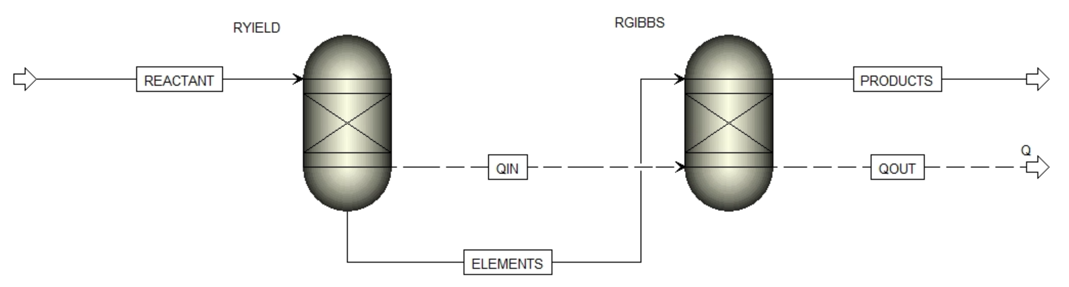
2.4. Aspen Plus Model
3. Results and Discussion
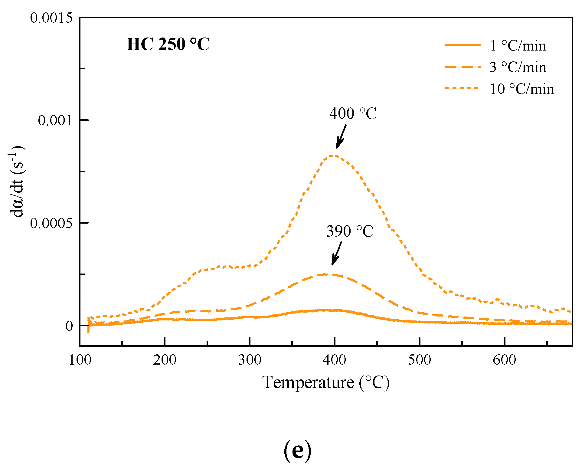
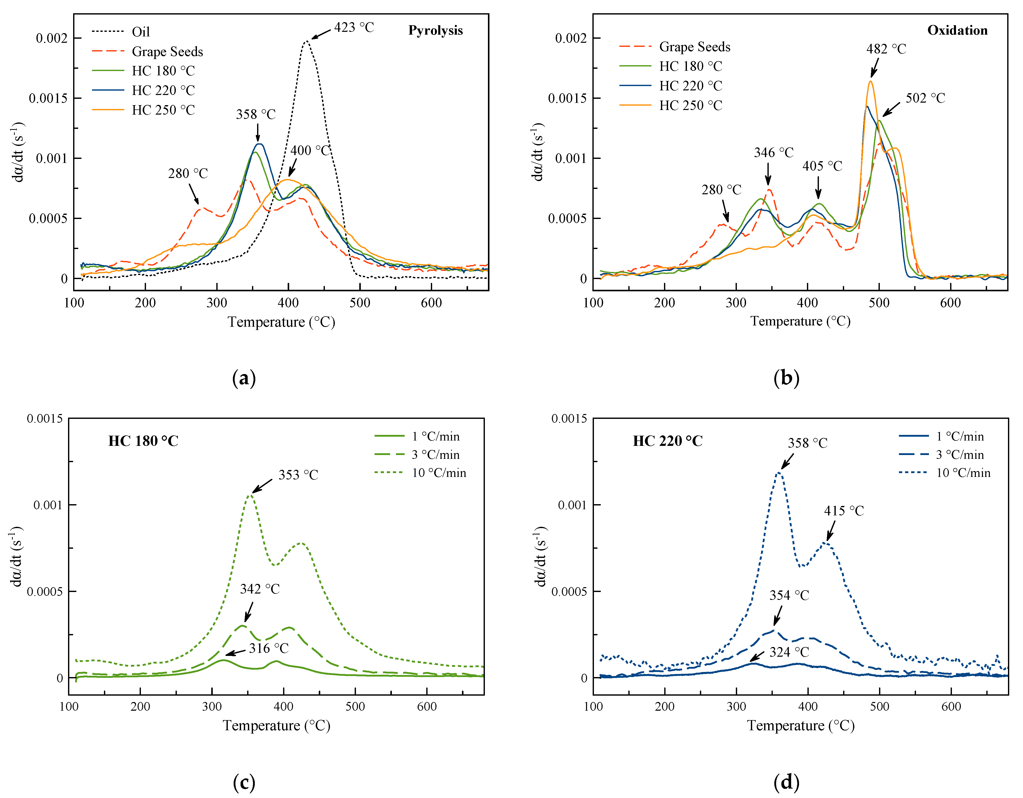
3.1. Derivative Thermogravimetric Curves
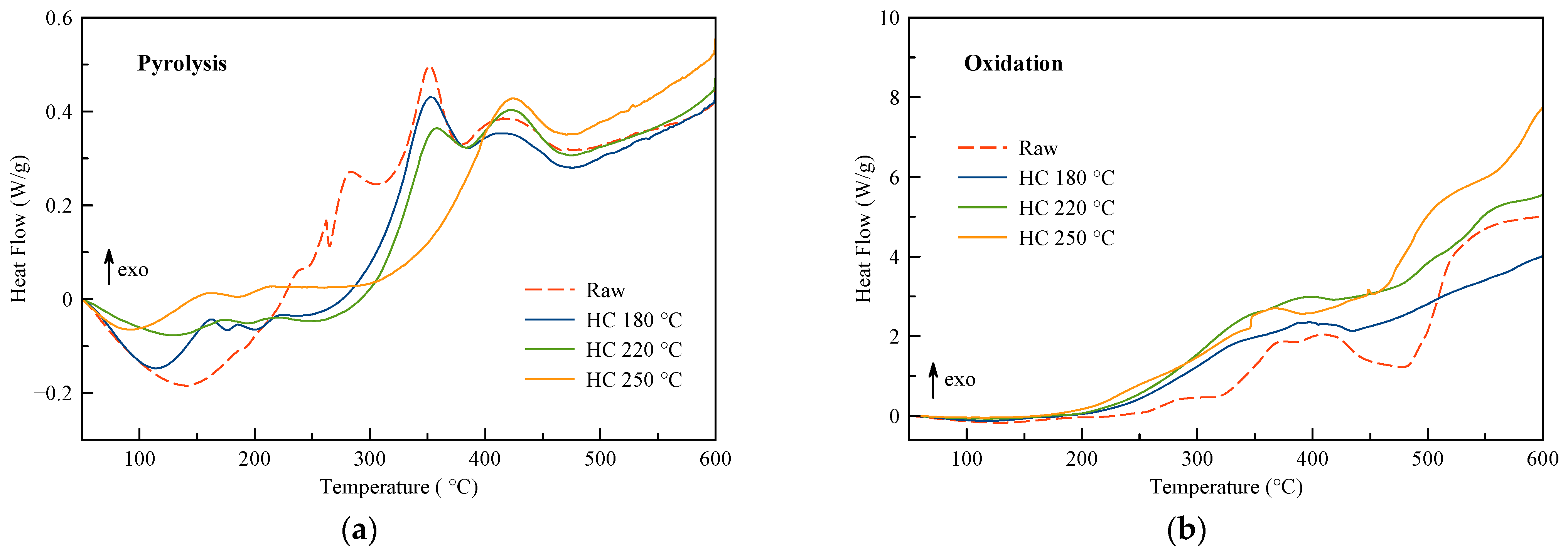
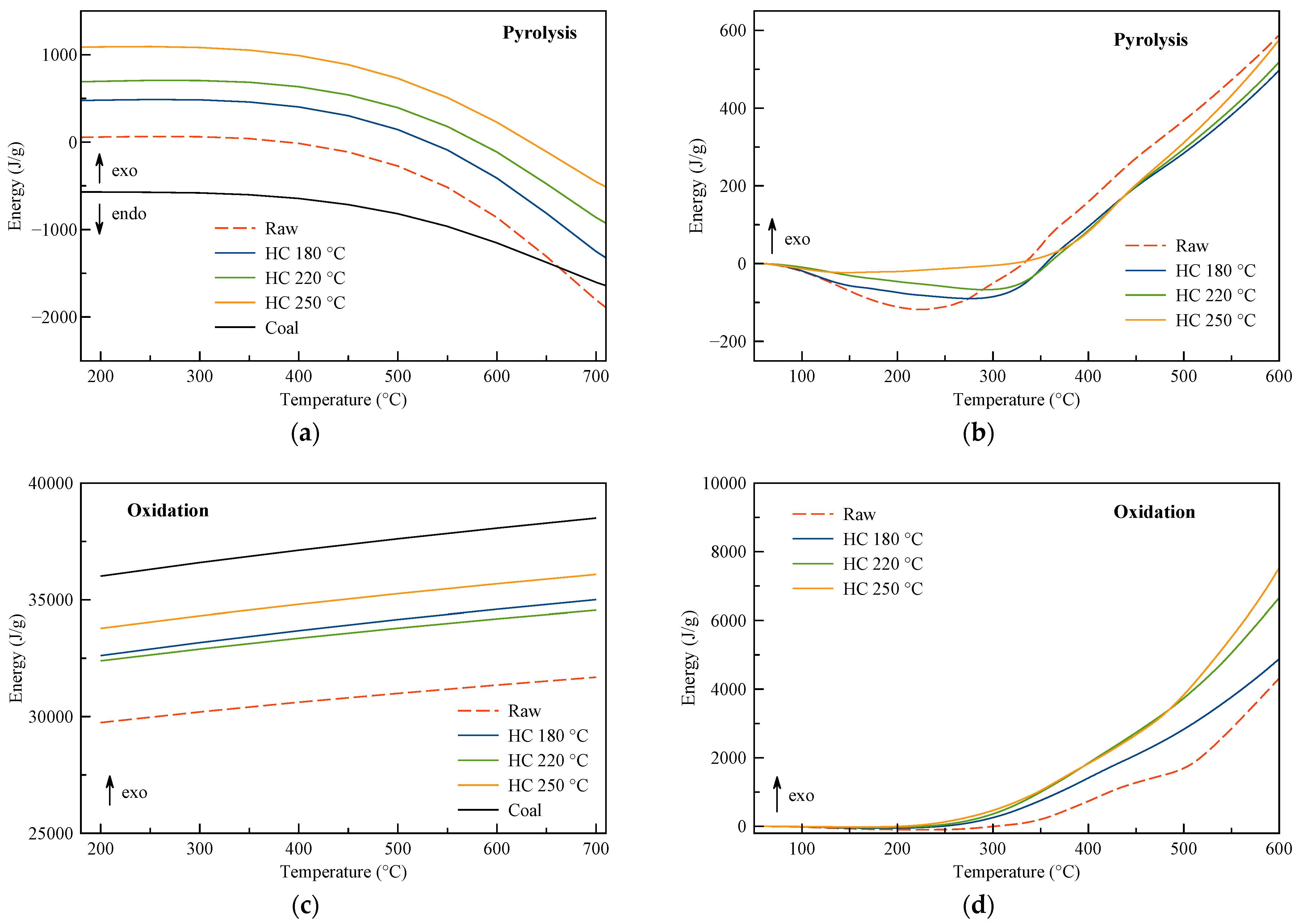
3.2. DSC Curves
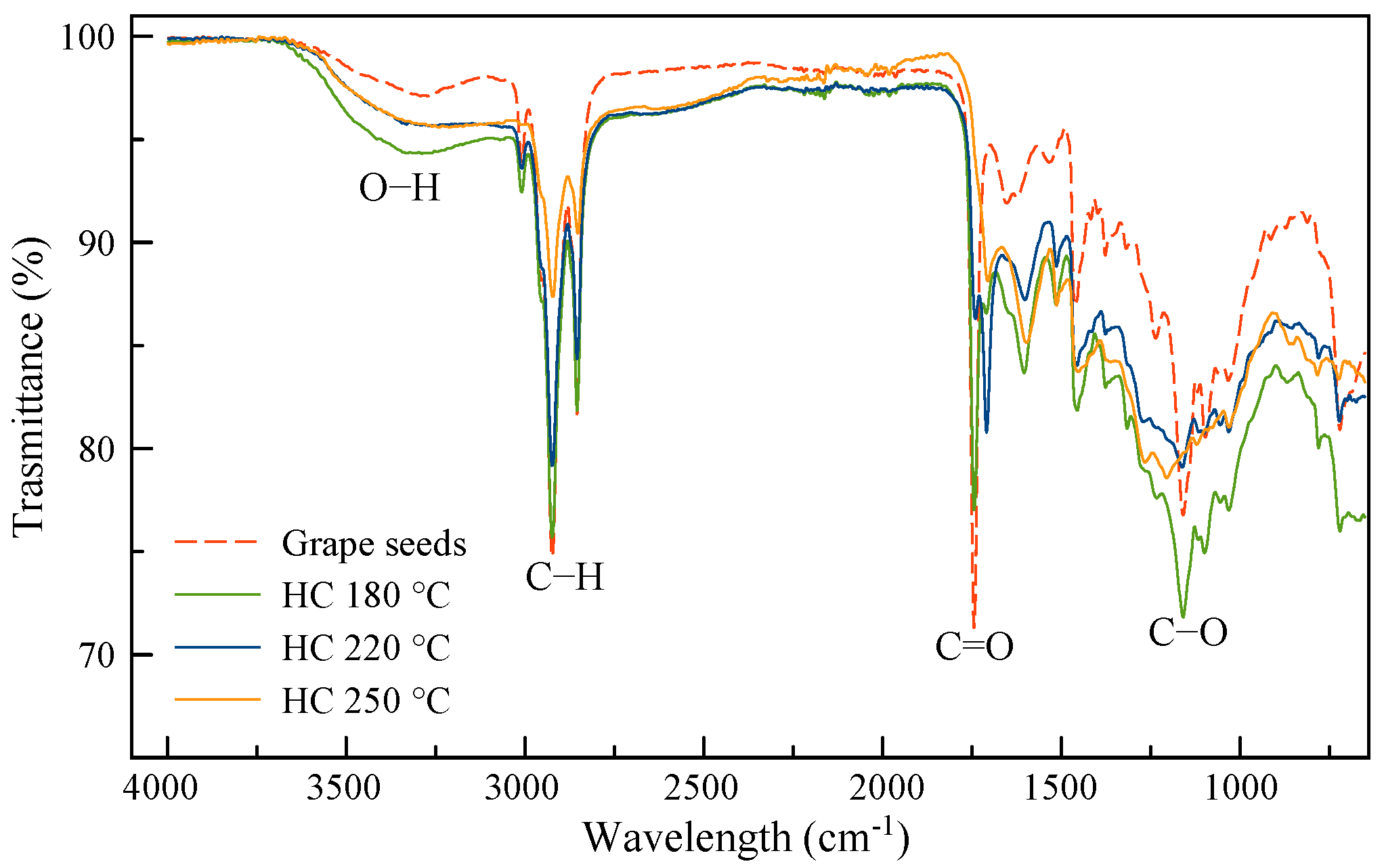
3.3. FTIR
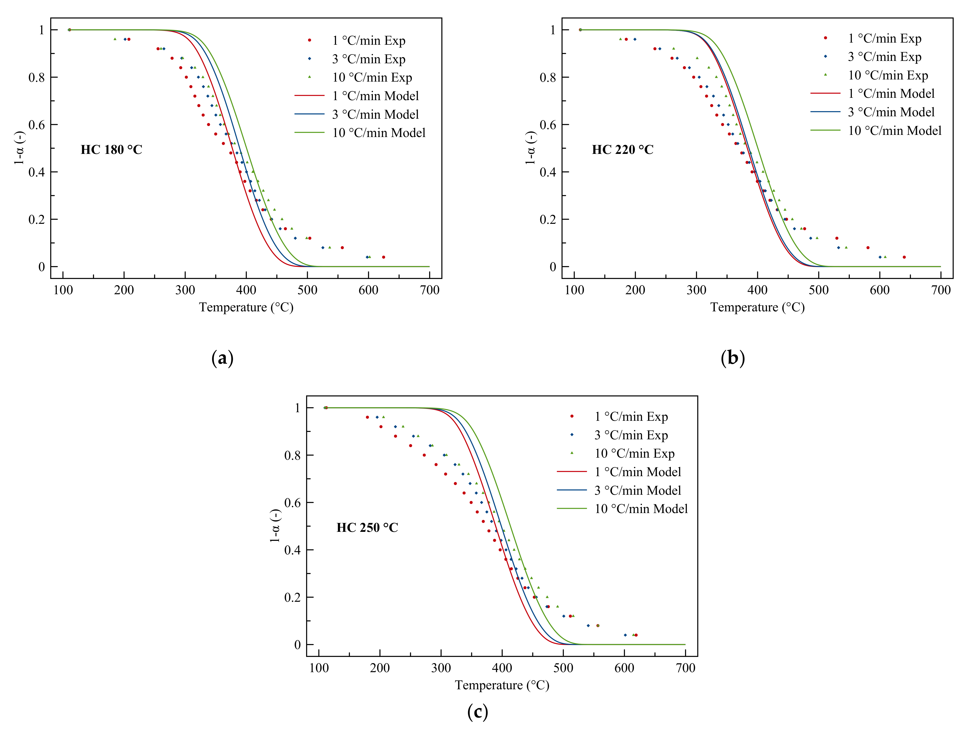
3.4. Kinetic Models
3.4.1. Gaussian Model
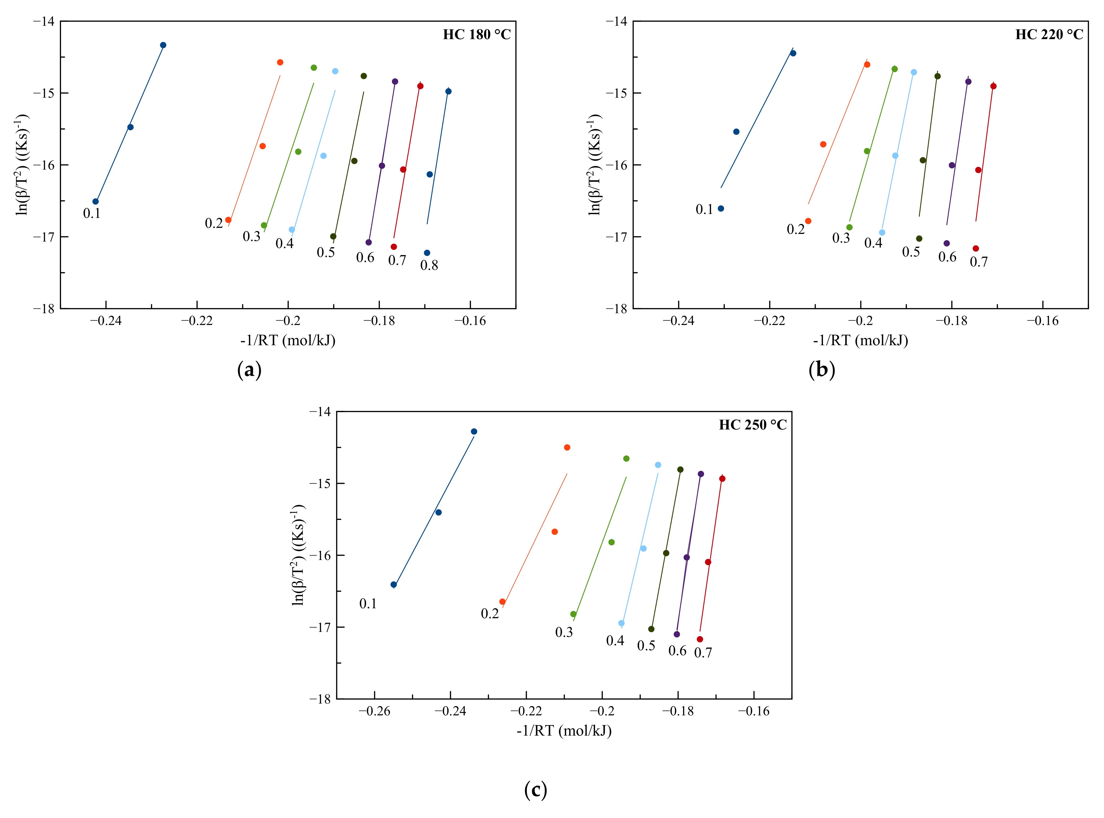
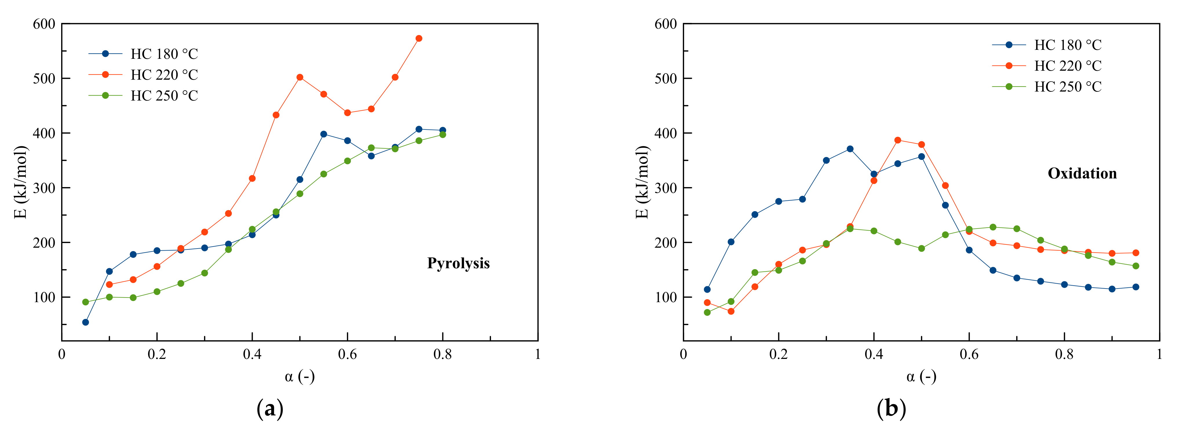
3.4.2. Miura–Maki Model
3.4.3. Comparison and Suggestions for Future Work
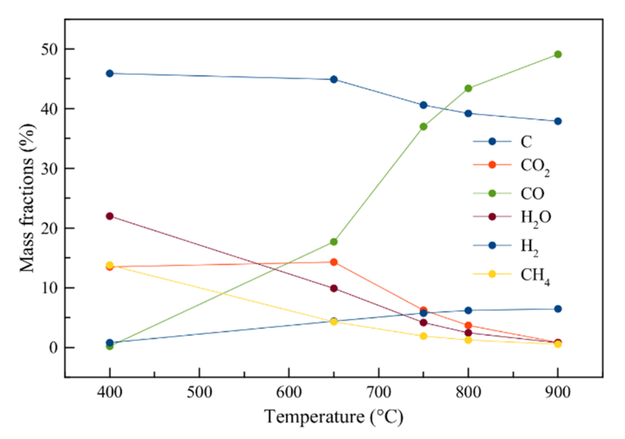
3.5. Aspen Plus Model
4. Conclusions
Supplementary Materials
Author Contributions
Funding
Institutional Review Board Statement
Informed Consent Statement
Data Availability Statement
Acknowledgments
Conflicts of Interest
References
- Li, J.; Pan, L.; Suvarna, M.; Tong, Y.W.; Wang, X. Fuel Properties of Hydrochar and Pyrochar: Prediction and Exploration with Machine Learning. Appl. Energy 2020, 269, 115166. [Google Scholar] [CrossRef]
- Ahmed, M.; Andreottola, G.; Elagroudy, S.; Negm, M.S.; Fiori, L. Coupling Hydrothermal Carbonization and Anaerobic Digestion for Sewage Digestate Management: Influence of Hydrothermal Treatment Time on Dewaterability and Bio-Methane Production. J. Environ. Manage. 2021, 281, 111910. [Google Scholar] [CrossRef] [PubMed]
- De Medeiros, A.D.M.; Da Silva Junior, C.J.G.; De Amorim, J.D.P.; Do Nascimento, H.A.; Converti, A.; De Santana Costa, A.F.; Sarubbo, L.A. Biocellulose for Treatment of Wastewaters Generated by Energy Consuming Industries: A Review. Energies 2021, 14, 1–18. [Google Scholar] [CrossRef]
- Yu, C.; Ren, S.; Wang, G.; Xu, J.; Teng, H.; Li, T.; Huang, C.; Wang, C.; Yu, C.; Ren, S.; et al. Kinetic Analysis and Modeling of Maize Straw Hydrochar Combustion Using a Multi- Gaussian-Distributed Activation Energy Model Kinetic Analysis and Modeling of Maize Straw Hydrochar Combustion Using a Multi-Gaussian-Distributed Activation. Energy Model. 2021, 28, 611–620. [Google Scholar]
- Zhang, N.; Wang, G.; Zhang, J.; Ning, X.; Li, Y.; Liang, W.; Wang, C. Study on Co-Combustion Characteristics of Hydrochar and Anthracite Coal. J. Energy Inst. 2020, 93, 1125–1137. [Google Scholar] [CrossRef]
- Chen, Z.; Hu, M.; Zhu, X.; Guo, D.; Liu, S.; Hu, Z.; Xiao, B.; Wang, J.; Laghari, M. Characteristics and Kinetic Study on Pyrolysis of Five Lignocellulosic Biomass via Thermogravimetric Analysis. Bioresour. Technol. 2015, 192, 441–450. [Google Scholar] [CrossRef]
- Chen, J.; Wang, Y.; Lang, X.; Ren, X.; Fan, S. Evaluation of Agricultural Residues Pyrolysis under Non-Isothermal Conditions: Thermal Behaviors, Kinetics, and Thermodynamics. Bioresour. Technol. 2017, 241, 340–348. [Google Scholar] [CrossRef]
- Ferrentino, R.; Merzari, F.; Fiori, L.; Andreottola, G. Coupling Hydrothermal Carbonization with Anaerobic Digestion for Sewage Sludge Treatment: Influence of HTC Liquor and Hydrochar on Biomethane Production. Energies 2020, 13, 6262. [Google Scholar] [CrossRef]
- Funke, A.; Ziegler, F. Hydrothermal Carbonization of Biomass: A Summary and Discussion of Chemical Mechanisms for Process Engineering. Biofuels, Bioprod. Biorefining 2010, 4, 160–177. [Google Scholar] [CrossRef]
- Olszewski, M.P.; Arauzo, P.J.; Wądrzyk, M.; Kruse, A. Py-GC-MS of Hydrochars Produced from Brewer’s Spent Grains. J. Anal. Appl. Pyrolysis 2019, 140, 255–263. [Google Scholar] [CrossRef]
- Ischia, G.; Cazzanelli, M.; Fiori, L.; Orlandi, M.; Miotello, A. Exothermicity of Hydrothermal Carbonization: Determination of Heat Profile and Enthalpy of Reaction via High-Pressure Differential Scanning Calorimetry. Fuel 2022, 310, 122312. [Google Scholar] [CrossRef]
- Ischia, G.; Fiori, L. Hydrothermal Carbonization of Organic Waste and Biomass: A Review on Process, Reactor, and Plant Modeling. Waste and Biomass Valorization 2021, 12, 2797–2824. [Google Scholar] [CrossRef]
- Scrinzi, D.; Andreottola, G.; Fiori, L. Composting Hydrochar-OFMSW Digestate Mixtures: Design of Bioreactors and Preliminary Experimental Results. Appl. Sci. 2021, 11, 1–15. [Google Scholar] [CrossRef]
- Lin, J.C.; Mariuzza, D.; Volpe, M.; Fiori, L.; Ceylan, S.; Goldfarb, J.L. Integrated Thermochemical Conversion Process for Valorizing Mixed Agricultural and Dairy Waste to Nutrient-Enriched Biochars and Biofuels. Bioresour. Technol. 2021, 328, 124765. [Google Scholar] [CrossRef]
- Hu, Q.; Yang, H.; Xu, H.; Wu, Z.; Lim, C.J.; Bi, X.T.; Chen, H. Thermal Behavior and Reaction Kinetics Analysis of Pyrolysis and Subsequent In-Situ Gasification of Torrefied Biomass Pellets. Energy Convers. Manag. 2018, 161, 205–214. [Google Scholar] [CrossRef]
- Román, S.; Libra, J.; Berge, N.; Sabio, E.; Ro, K.; Li, L.; Ledesma, B.; Alvarez, A.; Bae, S. Hydrothermal Carbonization: Modeling, Final Properties Design and Applications: A Review. Energies 2018, 11, 216. [Google Scholar] [CrossRef] [Green Version]
- Sharma, H.B.; Panigrahi, S.; Dubey, B.K. Hydrothermal Carbonization of Yard Waste for Solid Bio-Fuel Production: Study on Combustion Kinetic, Energy Properties, Grindability and Flowability of Hydrochar. Waste Manag. 2019, 91, 108–119. [Google Scholar] [CrossRef]
- Islam, M.A.; Kabir, G.; Asif, M.; Hameed, B.H. Combustion Kinetics of Hydrochar Produced from Hydrothermal Carbonisation of Karanj (Pongamia Pinnata) Fruit Hulls via Thermogravimetric Analysis. Bioresour. Technol. 2015, 194, 14–20. [Google Scholar] [CrossRef]
- He, C.; Giannis, A.; Wang, J.-Y. Conversion of Sewage Sludge to Clean Solid Fuel Using Hydrothermal Carbonization: Hydrochar Fuel Characteristics and Combustion Behavior. Appl. Energy 2013, 111, 257–266. [Google Scholar] [CrossRef]
- Bach, Q.V.; Tran, K.Q.; Skreiberg, Ø. Combustion Kinetics of Wet-Torrefied Forest Residues Using the Distributed Activation Energy Model (DAEM). Appl. Energy 2017, 185, 1059–1066. [Google Scholar] [CrossRef]
- Zhang, J.; Chen, T.; Wu, J.; Wu, J. Multi-Gaussian-DAEM-Reaction Model for Thermal Decompositions of Cellulose, Hemicellulose and Lignin: Comparison of N2 and CO2 Atmosphere. Bioresour. Technol. 2014, 166, 87–95. [Google Scholar] [CrossRef]
- Vand, V. A Theory of the Irreversible Electrical Resistance Changes of Metallic Films Evaporated in Vacuum. Proc. Phys. Soc. 1943, 55, 222–246. [Google Scholar] [CrossRef]
- Wang, S.; Dai, G.; Yang, H.; Luo, Z. Lignocellulosic Biomass Pyrolysis Mechanism: A State-of-the-Art Review. Prog. Energy Combust. Sci. 2017, 62, 33–86. [Google Scholar] [CrossRef]
- Radojević, M.; Janković, B.; Jovanović, V.; Stojiljković, D.; Manić, N. Comparative Pyrolysis Kinetics of Various Biomasses Based on Model-Free and DAEM Approaches Improved with Numerical Optimization Procedure. PLoS ONE 2018, 13, 1–25. [Google Scholar] [CrossRef]
- Hameed, S.; Sharma, A.; Pareek, V.; Wu, H.; Yu, Y. A Review on Biomass Pyrolysis Models: Kinetic, Network and Mechanistic Models. Biomass Bioenergy 2019, 123, 104–122. [Google Scholar] [CrossRef]
- White, J.E.; Catallo, W.J.; Legendre, B.L. Biomass Pyrolysis Kinetics: A Comparative Critical Review with Relevant Agricultural Residue Case Studies. J. Anal. Appl. Pyrolysis 2011, 91, 1–33. [Google Scholar] [CrossRef]
- Cai, J.; Wu, W.; Liu, R.; Huber, G.W. A Distributed Activation Energy Model for the Pyrolysis of Lignocellulosic Biomass. Green Chem. 2013, 15, 1331–1340. [Google Scholar] [CrossRef]
- Fiori, L.; Valbusa, M.; Lorenzi, D.; Fambri, L. Modeling of the Devolatilization Kinetics during Pyrolysis of Grape Residues. Bioresour. Technol. 2012, 103, 389–397. [Google Scholar] [CrossRef]
- Basso, D.; Weiss-Hortala, E.; Patuzzi, F.; Baratieri, M.; Fiori, L. In Deep Analysis on the Behavior of Grape Marc Constituents during Hydrothermal Carbonization. Energies 2018, 11, 1379. [Google Scholar] [CrossRef] [Green Version]
- Cai, J.M.; Bi, L.S. Kinetic Analysis of Wheat Straw Pyrolysis Using Isoconversional Methods. J. Therm. Anal. Calorim. 2009, 98, 325. [Google Scholar] [CrossRef]
- Branca, C.; Albano, A.; Di Blasi, C. Critical Evaluation of Global Mechanisms of Wood Devolatilization. Thermochim. Acta 2005, 429, 133–141. [Google Scholar] [CrossRef]
- Ischia, G.; Orlandi, M.; Fendrich, M.A.; Bettonte, M.; Merzari, F.; Miotello, A.; Fiori, L. Realization of a Solar Hydrothermal Carbonization Reactor: A Zero-Energy Technology for Waste Biomass Valorization. J. Environ. Manage. 2020. [Google Scholar] [CrossRef] [PubMed]
- Miura, K.; Maki, T. A Simple Method for Estimating f(E) and K0(E) in the Distributed Activation Energy Model. Energy and Fuels 1998, 12, 864–869. [Google Scholar] [CrossRef]
- Gao, L.; Volpe, M.; Lucian, M.; Fiori, L.; Goldfarb, J.L. Does Hydrothermal Carbonization as a Biomass Pretreatment Reduce Fuel Segregation of Coal-Biomass Blends during Oxidation? Energy Convers. Manag. 2019, 181, 93–104. [Google Scholar] [CrossRef]
- Miura, K. A New and Simple Method to Estimate f(E) and K0(E) in the Distributed Activation Energy Model from Three Sets of Experimental Data. Energy and Fuels 1995, 9, 302–307. [Google Scholar] [CrossRef]
- Coats, A.W.; Redfern, J.P. Kinetic Parameters from Thermogravimetric Data. Nature 1964, 201, 68–69. [Google Scholar] [CrossRef]
- Fischer, P.E.; Jou, C.S.; Gokalgandhi, S.S. Obtaining the Kinetic Parameters from Thermogravimetry Using a Modified Coats and Redfern Technique. Ind. Eng. Chem. Res. 1987, 26, 1037–1040. [Google Scholar] [CrossRef]
- Anthony, D.B.; Howard, J.B. Coal Devolatilization and Hydrogastification. AIChE J. 1976, 22, 625–656. [Google Scholar] [CrossRef]
- Güneş, M.; Güneş, S. A Direct Search Method for Determination of DAEM Kinetic Parameters from Nonisothermal TGA Data (Note). Appl. Math. Comput. 2002, 130, 619–628. [Google Scholar] [CrossRef]
- Ischia, G.; Fiori, L.; Gao, L.; Goldfarb, J.L. Valorizing Municipal Solid Waste via Integrating Hydrothermal Carbonization and Downstream Extraction for Biofuel Production. J. Clean. Prod. 2021, 289, 125781. [Google Scholar] [CrossRef]
- Spanghero, M.; Salem, A.Z.M.; Robinson, P.H. Chemical Composition, Including Secondary Metabolites, and Rumen Fermentability of Seeds and Pulp of Californian (USA) and Italian Grape Pomaces. Anim. Feed Sci. Technol. 2009, 152, 243–255. [Google Scholar] [CrossRef]
- Moldes, D.; Gallego, P.P.; Rodríguez Couto, S.; Sanromán, A. Grape Seeds: The Best Lignocellulosic Waste to Produce Laccase by Solid State Cultures of Trametes Hirsuta. Biotechnol. Lett. 2003, 25, 491–495. [Google Scholar] [CrossRef]
- Hubble, A.H.; Goldfarb, J.L. Synergistic Effects of Biomass Building Blocks on Pyrolysis Gas and Bio-Oil Formation. J. Anal. Appl. Pyrolysis 2021, 156, 105100. [Google Scholar] [CrossRef]
- Volpe, M.; Fiori, L. From Olive Waste to Solid Biofuel through Hydrothermal Carbonisation: The Role of Temperature and Solid Load on Secondary Char Formation and Hydrochar Energy Properties. J. Anal. Appl. Pyrolysis 2017, 124, 63–72. [Google Scholar] [CrossRef]
- Mackuľak, T.; Prousek, J.; Olejníková, P.; Bodík, I. Slovak Society of Chemical Engineering Institute of Chemical and Environmental Engineering Slovak University of Technology in Bratislava. Direct 2010, 1407–1412. [Google Scholar]
- Volpe, M.; Goldfarb, J.L.; Fiori, L. Hydrothermal Carbonization of Opuntia Ficus-Indica Cladodes: Role of Process Parameters on Hydrochar Properties. Bioresour. Technol. 2018, 247, 310–318. [Google Scholar] [CrossRef]
- Guo, S.; Dong, X.; Wu, T.; Shi, F.; Zhu, C. Characteristic Evolution of Hydrochar from Hydrothermal Carbonization of Corn Stalk. J. Anal. Appl. Pyrolysis 2015, 116, 1–9. [Google Scholar] [CrossRef]
- Purnomo, C.W.; Castello, D.; Fiori, L. Granular Activated Carbon from Grape Seeds Hydrothermal Char. Appl. Sci. 2018, 8, 1–16. [Google Scholar] [CrossRef] [Green Version]
- Diaz, E.; Manzano, F.; Villamil, J.A.; Rodriguez, J.; Mohedano, A. Low-Cost Activated Grape Seed-Derived Hydrochar through Hydrothermal Carbonization and Chemical Activation for Sulfamethoxazole Adsorption. Appl. Sci. 2019, 9, 5127. [Google Scholar] [CrossRef] [Green Version]
- Jiang, G.; Nowakowski, D.J.; Bridgwater, A.V. A Systematic Study of the Kinetics of Lignin Pyrolysis. Thermochim. Acta 2010, 498, 61–66. [Google Scholar] [CrossRef]
- Wang, S.; Ru, B.; Lin, H.; Sun, W.; Luo, Z. Pyrolysis Behaviors of Four Lignin Polymers Isolated from the Same Pine Wood. Bioresour. Technol. 2015, 182, 120–127. [Google Scholar] [CrossRef] [PubMed]
- Gomez, I.J.; Arnaiz, B.; Cacioppo, M.; Arcudi, F.; Prato, M. Nitrogen-Doped Carbon Nanodots for Bioimaging and Delivery of Paclitaxel. J. Mater. Chem. B 2018, 6, 5540–5548. [Google Scholar] [CrossRef] [PubMed] [Green Version]
- Cai, J.; Li, T.; Liu, R. A Critical Study of the Miura-Maki Integral Method for the Estimation of the Kinetic Parameters of the Distributed Activation Energy Model. Bioresour. Technol. 2011, 102, 3894–3899. [Google Scholar] [CrossRef] [PubMed]
- Xu, P.; Yu, B. The Scaling Laws of Transport Properties for Fractal-like Tree Networks. J. Appl. Phys. 2006, 100, 104906. [Google Scholar] [CrossRef] [Green Version]
- Liang, M.; Fu, C.; Xiao, B.; Luo, L.; Wang, Z. A Fractal Study for the Effective Electrolyte Diffusion through Charged Porous Media. Int. J. Heat Mass Transf. 2019, 137, 365–371. [Google Scholar] [CrossRef]
- Mäkelä, M.; Yoshikawa, K. Simulating Hydrothermal Treatment of Sludge within a Pulp and Paper Mill. Appl. Energy 2016, 173, 177–183. [Google Scholar] [CrossRef]
- Álvarez-Murillo, A.; Sabio, E.; Ledesma, B.; Román, S.; González-García, C.M. Generation of Biofuel from Hydrothermal Carbonization of Cellulose. Kinetics Modelling. Energy 2016, 94, 600–608. [Google Scholar] [CrossRef]


| Sample | Ultimate Analysis (wt.%) | Ash (wt.%) | HHV (MJ/kg) | ||||
|---|---|---|---|---|---|---|---|
| C | H | O | N | S | |||
| Grape seeds | 53.2 | 6.7 | 36.2 | 1.7 | 0.3 | 1.9 | 22.5 |
| HC 180 °C | 59.7 | 6.7 | 29.4 | 1.5 | 0.4 | 2.3 | 24.9 |
| HC 220 °C | 64.0 | 6.4 | 25.3 | 1.7 | 0.4 | 2.2 | 27.2 |
| HC 250 °C | 69.2 | 6.5 | 19.4 | 2.0 | 0.3 | 2.5 | 30.5 |
| Feedstock | Grape seeds, HC 180 °C, HC 220 °C, HC 250 °C, Coal |
| Products (at equilibrium) | C (graphite), CO2, CO, H2, O2, H2O, CH4, C2H2, C2H4, C2H6 |
| Equation of state | Peng–Robinson |
| Pyrolysis temperature | 300–900 °C |
| DTGA Peak | Pyrolysis | Oxidation | ||||||||
|---|---|---|---|---|---|---|---|---|---|---|
| Oil | Grape Seeds | HC 180 °C | HC 220 °C | HC 250 °C | Grape Seeds | HC 180 °C | HC 220 °C | HC 250 °C | ||
| 1 | T (°C) | - | 280 | - | - | - | 280 | - | - | - |
| dα/dt (s−1) | - | 5.9 × 10⁻⁴ | - | - | - | 4.4 × 10⁻⁴ | - | - | - | |
| 2 | T (°C) | - | 343 | 353 | 358 | - | 346 | 334 | 336 | - |
| dα/dt (s−1) | - | 8.2 × 10⁻⁴ | 1.0 × 10⁻³ | 1.1 × 10⁻³ | - | 7.4 × 10⁻⁴ | 6.6 × 10⁻⁴ | 5.7 × 10⁻⁴ | - | |
| 3 | T (°C) | 423 | 421 | 424 | 428 | 400 | 415 | 415 | 406 | 409 |
| dα/dt (s−1) | 2.0 × 10⁻³ | 6.6 × 10⁻⁴ | 7.8 × 10⁻⁴ | 7.7 × 10⁻⁴ | 8.2 × 10⁻⁴ | 4.6 × 10⁻⁴ | 6.2 × 10⁻⁴ | 5.8 × 10⁻⁴ | 5.3 × 10⁻⁴ | |
| 4 | T (°C) | - | - | - | - | - | 502 | 502 | 482 | 480–523 |
| dα/dt (s−1) | - | - | - | - | - | 1.1 × 10⁻³ | 1.3 × 10⁻³ | 1.4 × 10⁻³ | 1.6–1.1 × 10⁻³ | |
| Pyrolysis | Oxidation | |||||||
|---|---|---|---|---|---|---|---|---|
| Raw | HC 180 °C | HC 220 °C | HC 250 °C | Raw | HC 180 °C | HC 220 °C | HC 250 °C | |
| Endothermic 1 (J/g) | 118 | 90 | 67 | 23 | 98 | 54 | 31 | 19 |
| Exothermic 1 (J/g) | 705 | 587 | 585 | 598 | 4406 | 4928 | 6678 | 7533 |
| Net energy 1 (J/g) | 587 | 497 | 518 | 575 | 4309 | 4874 | 6647 | 7514 |
| Mass loss 1 (%) | 61.2 | 56.2 | 55.4 | 43.7 | 73.7 | 69.0 | 73.3 | 69.0 |
| Grape Seeds | Oil | HC 180 °C | HC 220 °C | HC 250 °C | |||
|---|---|---|---|---|---|---|---|
| Pyrolysis | E0 (kJ/mol) | 1 °C/min | - | - | 205 | 207 | 209 |
| 3 °C/min | - | - | 203 | 202 | 206 | ||
| 10 °C/min | 193 | 218 | 200 | 200 | 204 | ||
| σ (kJ/mol) | 1 °C/min | - | - | 15 | 16 | 17 | |
| 3 °C/min | - | - | 14 | 15 | 16 | ||
| 10 °C/min | 16 | 11 | 15 | 15 | 16 | ||
| h (-) | 1 °C/min | - | - | 0.083 | 0.090 | 0.089 | |
| 3 °C/min | - | - | 0.061 | 0.072 | 0.073 | ||
| 10 °C/min | 0.084 | 0.022 | 0.064 | 0.062 | 0.076 | ||
| Oxidation | E0 (kJ/mol) | 1 °C/min | - | - | 211 | 214 | 219 |
| 3 °C/min | - | - | 215 | 215 | 220 | ||
| 10 °C/min | 213 | - | 214 | 213 | 221 | ||
| σ (kJ/mol) | 1 °C/min | - | - | 14 | 15 | 15 | |
| 3 °C/min | - | - | 15 | 14 | 15 | ||
| 10 °C/min | 17 | - | 16 | 15 | 15 | ||
| h (-) | 1 °C/min | - | - | 0.057 | 0.065 | 0.065 | |
| 3 °C/min | - | - | 0.071 | 0.066 | 0.066 | ||
| 10 °C/min | 0.102 | - | 0.084 | 0.077 | 0.077 | ||
| Model | Atmosphere | Parameter | Grape Seeds | Oil | Hydrochar | ||
|---|---|---|---|---|---|---|---|
| 180 °C | 220 °C | 250 °C | |||||
| Gaussian | Pyrolysis | E (kJ/mol) | 193 | 218 | 203 | 203 | 206 |
| σ (kJ/mol) | 16 | 11 | 15 | 15 | 16 | ||
| Oxidation | E (kJ/mol) | 213 | - | 213 | 214 | 220 | |
| σ (kJ/mol) | 17 | - | 15 | 15 | 15 | ||
| Miura-Maki | Pyrolysis | E (kJ/mol) | - | - | 265 | 339 | 239 |
| k0 (s−1) | - | - | 7.6 × 1027 | 6.0 × 1038 | 9.8 × 1024 | ||
| Oxidation | E (kJ/mol) | - | - | 222 | 215 | 181 | |
| k0 (s−1) | - | - | 3.4 × 1026 | 1.0 × 1026 | 2.9 × 10¹³ | ||
Publisher’s Note: MDPI stays neutral with regard to jurisdictional claims in published maps and institutional affiliations. |
© 2022 by the authors. Licensee MDPI, Basel, Switzerland. This article is an open access article distributed under the terms and conditions of the Creative Commons Attribution (CC BY) license (https://creativecommons.org/licenses/by/4.0/).
Share and Cite
Gonnella, G.; Ischia, G.; Fambri, L.; Fiori, L. Thermal Analysis and Kinetic Modeling of Pyrolysis and Oxidation of Hydrochars. Energies 2022, 15, 950. https://doi.org/10.3390/en15030950
Gonnella G, Ischia G, Fambri L, Fiori L. Thermal Analysis and Kinetic Modeling of Pyrolysis and Oxidation of Hydrochars. Energies. 2022; 15(3):950. https://doi.org/10.3390/en15030950
Chicago/Turabian StyleGonnella, Gabriella, Giulia Ischia, Luca Fambri, and Luca Fiori. 2022. "Thermal Analysis and Kinetic Modeling of Pyrolysis and Oxidation of Hydrochars" Energies 15, no. 3: 950. https://doi.org/10.3390/en15030950
APA StyleGonnella, G., Ischia, G., Fambri, L., & Fiori, L. (2022). Thermal Analysis and Kinetic Modeling of Pyrolysis and Oxidation of Hydrochars. Energies, 15(3), 950. https://doi.org/10.3390/en15030950