Forecasting Solar Home System Customers’ Electricity Usage with a 3D Convolutional Neural Network to Improve Energy Access

Abstract

Off-grid technologies, such as solar home systems (SHS), offer the opportunity to alleviate global energy poverty, providing a cost-effective alternative to an electricity grid connection. However, there is a paucity of high-quality SHS electricity usage data and thus a limited understanding of consumers’ past and future usage patterns. This study addresses this gap by providing a rare large-scale analysis of real-time energy consumption data for SHS customers (n = 63,299) in Rwanda. Our results show that 70% of SHS users’ electricity usage decreased a year after their SHS was installed. This paper is novel in its application of a three-dimensional convolutional neural network (CNN) architecture for electricity load forecasting using time series data. It also marks the first time a CNN was used to predict SHS customers’ electricity consumption. The model forecasts individual households’ usage 24 h and seven days ahead, as well as an average week across the next three months. The last scenario derived the best performance with a mean squared error of 0.369. SHS companies could use these predictions to offer a tailored service to customers, including providing feedback information on their likely future usage and expenditure. The CNN could also aid load balancing for SHS based microgrids.

1. Introduction

Globally, 770 million people had no access to electricity in 2019, of which 75% lived in Sub-Saharan Africa [1]. Considering that energy is vital to the functioning of many services, including health and education, urgent action is needed to increase current energy access levels. Consequentially, the United Nations proposed Sustainable Development Goal 7, aiming for affordable and clean energy for all by 2030 as part of the Paris Agreement [2]. Households tend to gain energy access by connecting to the national electricity grid or via off-grid energy technologies. The off-grid energy market has grown in recent years, offering energy access to rural low density populations that are unable to afford an electricity grid connection or live outside the grid’s vicinity [3].

This study focusses on solar home system (SHS) customers, who have multiplied in recent years, with over 30 million SHSs purchased globally since 2010, particularly in Sub-Saharan Africa [4]. A SHS consists of a solar panel and battery and includes appliances, such as radios [5]. Their growth over recent years is partly due to innovate business models, such as pay-as-you-go (PAYG), which eased the affordability barrier faced by many households. PAYG models allow individuals to only pay for days of electricity when they can afford to, thus offering payment flexibility. Several countries, including Rwanda, are relying on SHSs as part of their electrification strategy [6]. Being considered a key contender in providing energy access, it is important to better understand SHS users and their experiences [7]. The literature on SHS consumption patterns and electricity load forecasting has been particularly sparse, likely due to the paucity of high-quality data. Only a few studies explored SHS electricity consumption data directly derived from SHSs. Gustavsson [8] examined Zambian SHS customers’ usage through data loggers, finding that SHS usage was mainly concentrated in the morning and evenings. However, their analysis was based on only three users. Opoku et al. [9] studied the SHS consumption patterns of one Ghanaian household, discovering key differences in weekday and weekend consumption, as well as the importance of maximising electricity use directly from the solar panel. Another key study by Bisaga and Parikh [10] examined 217 Rwandan customers’ SHS electricity usage for three months, finding the group of customers with the fewest appliances to consistently use more energy than groups with more appliances. Bhatti and Williams [11] investigated electricity load data from four SHS households in India and discovered that half of the solar energy produced was surplus energy. Although, these studies provide important insights into usage patterns, there is room for analysis on larger customer samples and a longer time period. Electricity load forecasting of SHS-derived data is still nascent, where Manur et al. [12] published one of the first papers on this topic. Although, they only examined one SHS customer in India using a long short-term memory model. This study will aim to address the gaps in both the SHS electricity consumption analysis and forecasting literature through a case study of SHS users in Rwanda using real-time electricity usage data from a SHS provider.

2. Literature Review

Electricity load forecasting has become common practice and is considered crucial in many sectors. The government utilises long-term forecasting to plan for future capital investment and utilities may use short-term forecasting to enable demand-response planning [13,14]. With the advent of more decentralised renewable energy, such as wind or solar energy, powering the grid, accurate forecasting is becoming more important, due to their intermittent nature [15]. The literature on electricity load forecasting for individual households has particularly flourished in recent years. In developed countries, this is partly due to the increased usage of smart meters that record electricity usage of individuals in real-time [16]. Predicting future electricity demand for residential purposes enables electricity generators, distributors and suppliers to effectively plan ahead. It can also promote energy conservation amongst users, as they become aware of their own energy demand. Forecasting at an individual level can be more challenging than aggregate predictions, due to the accompanying data volatility. Consumption can be influenced by a wide variety of factors, including “devices’ operational characteristics, users’ behaviours, economic factors, time of the day, day of the week, holidays, weather conditions, geographic patterns and random effects” [17]. Therefore, individuals’ consumption can vary considerably from one another, which makes forecasting more difficult.

Differences between developed and developing nations’ electricity consumption can be observed. For instance, electricity loads are much lower in African households, which also tend to have fewer appliances compared to households in high-income nations [18]. Moreover, the electricity grid is often unreliable in developing countries, with households experiencing frequent outages [19]. There is a high concentration of decentralised technologies, including SHSs, particularly amongst the off-grid population in developing countries. Gaining access to consumption data from these technologies is difficult, as only a few companies measure this data and may be unwilling to share it to protect their intellectual property. These factors influence the ability to forecast electricity consumption of off-grid users in developing countries. Electricity usage of SHSs can also be highly variable due to the intermittency of the energy supply and battery capacity limitations that can result in individuals running out of battery [8,12]. Another factor that contributes to this intermittency is the dominance of PAYG payments that enable individuals to only pay for electricity usage when they can afford to. This results in periods of time, where no electricity is consumed. These factors can make forecasting more challenging than for households in developed countries. This study aims to highlight that forecasting multiple individual SHS customers’ consumption in developing countries is possible and important to better cater to their specific needs.

2.1. Common Load Forecasting Models

A number of load forecasting models are used in the energy domain to predict individuals’ consumption, which include regression-based, ARIMA, grey, fuzzy logic, artificial neural networks and support vector machines (

Table 1. Description of various load forecasting models and their application (adapted from [20]). Adapted with permission from ref. [20]. Copyright 2018 Elsevier.

Models	Feature	Advantages	Disadvantages
Regression-based	Find out influencing factors; build the regression equation between factors and objectives	Good at analysing multi-factor models; provide error checking of model estimation parameters; easy to calculate	Does not consider the un-testability of certain influence factors; results cannot reflect periodic wave
ARIMA	Established by regression of the dependent variable only for its lag value and the present value of the random error term	The mathematical model requires only endogenous variables without resorting to exogenous variables	Require timing data to be stable; cannot reflect non-linear relationships; the determination of model parameters is complicated
Fuzzy Logic	Perform fuzzy judgment for systems with unknown models; reasoning solves the regular fuzzy information problem that is difficult to deal with by conventional methods	High accuracy in reflecting uncertainty qualitative knowledge; good at uncertain situation prediction of input variables	Lack of specific prediction formulas; cannot reflect the relationship between predicted values and historical data
Artificial Neural Networks	It abstracts the human brain neural network from the perspective of information processing; usually a logical expression of some kind of algorithm in nature.	Provide self-learning function and high-speed search for optimal solutions; fully approximate any arbitrarily complex non-linear relationship; can learn and adapt to unknown or uncertain systems	No ability to explain reasoning process and reasoning basis; cannot work when data is insufficient; turning all reasoning into numerical calculations results in the loss of information
Support Vector Regression	Find the best compromise between the complexity of the model and the learning ability based on limited sample information	Can solve machine learning and non-linear problems in the case of small samples; simplify the usual classification and regression issues; can improve generalization performance; less parameters to solve	Sensitive to missing data; difficult to implement large-scale training samples; difficult to solve multiple classification problem

).

The method chosen is highly dependent on the data characteristics, number of variables and the forecast period. Forecasting time periods can be split into very short-term, short-term, medium-term and long-term, where the amount of time for each differs depending on the sector. Long-term predictions cover any period over a year and medium-term constitutes the period between a month and a season [21]. Short-term forecasting refers to an hour to several days, whilst very short-term is less than an hour [21]. This study specifically examines short- and medium-term forecasting. Wang et al. [20] highlighted which models were optimal, in terms of predictive performance, based on the data characteristics (

Table 2. Comparison of model’s predictive performance (adapted from [20]). Adapted with permission from ref. [20]. Copyright 2018 Elsevier.

Models	Data Trend Characteristics		Forecast Period		Number of Variables		Most Applied Case in Energy Field
	Linear	Non-Linear	Long-Term	Short-Term	Multivariate	Univariate
Regression-based							Short-term load forecasting
ARIMA							Electricity price/energy consumption
Fuzzy Logic							Short-term electricity consumption
Artificial Neural Networks							Electricity price/energy consumption
Support Vector Regression							Hourly/daily/monthly load demand

Note: The symbol means the relative superiority of predictive performance.

).

This research utilised a discrete multivariate time series with non-linear data. The aim was to forecast short- and medium-term electricity usage of individual SHS customers. Based on Table 2, an ANN or Fuzzy Logic model would be ideal. An ANN was chosen partly due to the large dataset available, which suits ANN’s learning ability [22]. This dataset also does not fit the fuzzy logic model, which normally deals with vague information [23]. ANNs have several advantages, which include being able to understand non-linear relationships between variables and reducing the need for feature engineering due to its reliance on the universal approximation theorem [24,25]. The diminished need for feature engineering is particularly useful in a developing country context, as it enables less reliance on external often difficult to access data. Several ANN types have been used for electricity load forecasting, where popular ones include multi-layer perceptron (MLP), long short-term memory (LSTM) and convolutional neural network (CNN). This study chose a CNN as it benefits from greater context for feature extraction due to its stacked layers, allowing the data structure to be kept intact [26]. Moreover, a CNN faces fewer computational challenges than MLP and LSTM, due to its local connectivity feature that allows for weight sharing and the limited use of fully connected layers [26]. Finally, the CNN can be trained more quickly than an LSTM, for instance, as it can run concurrently [27]. This study will utilise a CNN for short- and medium-term electricity load forecasting for SHS customers.

A few studies have used CNNs to predict electricity consumption of individual households. Acharya et al. [28] forecasted households in Korea using a one-dimensional CNN, which performed better than the LSTM when utilising augmented data. A French household’s usage for the subsequent 60 h was predicted by Amarasinghe et al. [29] with a CNN, which fared better than their Support Vector Machine and was comparable in performance to LSTM with sequence to sequence. Lang et al. [30] forecasted the next 36 h of Irish households’ electricity usage using a CNN, highlighting the effectiveness of a simple architecture. The CNN’s prediction of a solar photovoltaic system’s consumption in the next 30 min in an Australian study was better than the LSTM and MLP model outcomes for the same dataset [31]. Finally, Heo et al. [32] forecasted solar power output in South Korea for the next month using a multi-channel CNN to extract more features. These studies all utilise a one-dimensional CNN architecture. In contrast, three-dimensional (3D) CNNs have not yet been trialled for electricity load forecasting of time series data, as far as the authors could see. A 3D architecture enables the data structure to remain intact, thereby providing valuable spatial information that could improve the CNN’s prediction capability.

2.2. Intervention Research

Electricity load predictions of individual households help utilities offer relevant time-of-use tariffs and assists load management purposes [33]. These forecasts also enable providers or policymakers to intervene, in order to spark behaviour change in users. There has been a recent focus on reducing electricity usage, particularly at peak hours to reach emission targets in developed nations [34,35]. In countries where energy access levels are low though, there has been a concerted effort to electrify households and to ensure their electricity amount can satisfy their energy needs reliably.

Individuals’ electricity consumption could be influenced through behavioural interventions, such as “commitment, goal setting, providing information, reward [and] result feedback” [36]. Bonan et al. [37] studied how households’ PAYG repayments for off-grid electricity are affected by setting commitments, finding that a combination of commitment and PAYG flexibility was better than a strict schedule to lower the number of defaults in the long term. Interventions, such as information and feedback, place more emphasis on the electricity provider. Gaining information relates to more general advice, whilst feedback refers to specific tips to change behaviour, tailored to an individuals’ electricity usage profile [36,38]. Smart meters that highlight the electricity used in a house in real time, offer households such feedback, where multiple studies found their installation to have reduced electricity consumption, usually in the short-term [16,39]. Normative feedback, which involves informing a specific household how their energy usage differs to that of others, has been shown as especially constructive [16,40]. Load forecasting could be used to provide feedback information that potentially leads to behaviour change. This information enables households to become aware of their future usage and manage their upcoming expenditure [41]. However, the literature on interventions based on forecasted data is limited. Electricity usage data from smart homes was used by Chen and Cook [42] to train a linear regression and SVR model, the results of which were then accessible to both households. However, future research is needed to understand whether this feedback induces behaviour change and the longevity of this effect.

SHS providers and policymakers may use load forecasting to help make proactive decisions and provide feedback to consumers. SHS companies can analyse their customers’ past and predicted consumption to spot trends on whether a households’ usage is on an upward or downward trend. SHS consumers could then benefit from receiving a more tailored service from their provider based on their individual profile. Households could also react to a company’s feedback. For instance, if customers were informed in which hours they use their SHS extensively, it may help them reduce occasions they run out of battery. Moreover, being aware of their likely usage can help households better plan their future expenditure and thus lower their likelihood of defaulting on payments and losing their SHS. Microgrid operators that connect multiple SHSs to each other, could use the electricity consumption forecasts for load balancing purposes to limit outages [43]. Finally, it can be helpful for policymakers to examine past SHS usage data and load forecasts to help pinpoint regions well suited for electricity grid expansion or microgrids.

2.3. Gaps in Literature

Despite research on SHS usage rising over recent years, a number of gaps remain in the literature [44]. One of these is a lack of analysis on SHS usage patterns, with the limited studies on this subject often examining self-reported data, for instance in the Opiyo [45] study. Such self-reported data is normally recorded at seldom intervals or the respondent is asked to estimate an average, thereby making the data less precise. Only a few studies explored electricity consumption data directly derived from SHSs [8,9,10,11]. There is a need for more SHS analysis on larger customer samples and a longer time period, which this study will address, thereby aiming to provide more generalisable findings. There are limited load forecasting models that concern individual households in developing countries. Much of the existing literature focusses on developed nations, which operate in a different context, usually centred on electricity grid consumers. The SHS consumption forecasting sector is particularly nascent, where a study by Manur et al. [12] was the only paper discovered to tackle this issue. They used an LSTM to predict the next hour’s usage of a single SHS customer in India. Finally, as discussed in Section 2.1, the lack of 3D CNNs for load forecasting based on time series data should be addressed. 3D CNNs have become the norm in image classification; however, this architecture should also be explored more extensively in wider use cases, including load forecasting for individuals.

3. Materials and Methods

This study utilised data from a solar energy provider, Bboxx, which operates in 11 countries across Africa and Asia. They sell ‘smart’ SHSs, which have a sim card that transfers data about the SHS on a millisecond scale back to their headquarters [46]. The company offers SHSs with different capacity sizes, including 20-, 50- and 300-Watt (W) SHSs. Bboxx uses a hybrid rent-to-own and fee-for-service business model to cater to the low-income population, which are often unable to pay for a SHS outright [47,48,49]. This involves households paying an initial down payment, followed by regular instalments over a three-year period, at the end of which they own the accompanying appliances, but not the solar panel or battery. After three years, the household pays an ‘Energy Service Fee’ whenever they want to use electricity, for which they receive continued access to maintenance services. The company offers customers a PAYG payment option, as long as they pay for a set minimum number of days. This research focusses specifically on customers in Rwanda using a 50 W SHS, which was the company’s first country of operation and type of SHS, respectively, thus this combination resulted in the most data to examine.

This study utilises a time series analysis and CNN to investigate SHS users’ past and future electricity consumption patterns. The two methods examined different time periods. Overall, only data until March 2020 was used to avoid any potential impact of the COVID-19 pandemic on the electricity usage data. The CNN was tested on various input time periods, starting with the one in

Table 3. Dates and number of customers per method.

Method	Dates	Number of Customers
Time series analysis	1 March 2019–29 Feburary 2020	63,299
CNN	11 Feburary 2019–29 December 2019	48,485

, which comprised six months as input and three months as output. However, the CNN’s forecasting ability improved with a lower input period of 17 weeks, which was thus used to derive the results presented in this study.

Both methods utilised Python 3.7 and for the CNN PyTorch 1.6 was used as the machine learning framework.

3.1. Time Series Analysis

A time series analysis was conducted to gain insights on the electricity usage behaviour of SHS customers. Specifically, the yearly, monthly and weekly patterns were examined. The Wilcoxon signed-rank test was used to investigate whether the weekday and weekend samples derived from different distributions, where a p-value of below 0.05 was deemed significant. The customers were also placed into groups depending on which appliances they owned. The SHS provider offered the following appliances: torches, bulbs, shavers, radios and televisions. After examining the electricity consumption data, the clearest distinction in usage was visible between television owners and households without a television. Additional appliances did not have a considerable impact on this divide. Therefore, the time series analysis focussed specifically on television and non-television owners (

Table 4. Number of customers and average daily electricity consumption per group.

Groups	Customers	Percent (%)	Mean Daily Electricity Usage (Wh)
No television	56,166	90	43.2
Television	6291	10	66.3
	62,457	100

).

Individual SHS users’ consumption at different stages across a year was examined to better understand their customer journey. Specifically, households that became active customers between February and March 2019, which owned a television (n = 219) and ones without a television (n = 2288). Each household’s total electricity usage was calculated a month after their SHS was installed and then compared to their consumption in three, six, nine and twelve months’ time. A t-test for paired samples was performed to see whether the difference in electricity usage from the first month to each of these subsequent months was statistically significant, where the significance level was 0.05. This analysis provides a valuable insight into how electricity usage of individual households tends to change over time, highlighting when customers may require additional support.

3.2. CNN

3.2.1. CNN Architecture

A multivariate 3D CNN was developed for this research to predict short- and medium-term electricity consumption of SHS customers. The model development process is highlighted in Figure 1, which outlines the splitting of data and the individual model steps, which proceed in a largely linear manner, with the exception of two loops.

Figure 1 highlights that the first step was to clean the SHS electricity consumption data, which included removing households that had not used their SHS for a minimum of three months and patching implausible electricity and temperature data for specific timestamps. The cleaned data was split into individual training, validation and test datasets. Each of these datasets were pre-processed before being loaded into the model, which involved reshaping the data, so it had the required number of dimensions. The electricity usage and temperature values were normalised before the initial hyperparameters of the CNN were specified and the weights initialised. The training data was shuffled before the model was trained on batches of the dataset. The initial loop in Figure 1 details whether the network has converged or in other words whether the loss has stopped reducing and is stable. The loss function used to train the CNN was the mean absolute error (MAE), which quantifies the absolute difference between the model’s forecasts and the true values [50]. The model calculates the MAE for each batch of input data received and the adaptative moment estimation (Adam) optimiser uses this to effectively adjust the weights to reduce the loss, thereby training the model. The second loop in Figure 1 is activated if the model performance is unsatisfactory, which leads to the hyperparameters being changed and the weights being initialised again to train the model anew. The hyperparameter values have to be set by the researcher prior to training and are key, as they influence the learning process and the model’s shape [51]. If the CNN performance is satisfactory, the model is saved and to highlight its generalisability, it is trialled on an unseen test dataset.

This study shows the first 3D CNN architecture utilised for load forecasting based on time series data, as far as the authors are aware. This design enables the CNN to make use of the spatial dimensions to determine temporal patterns, as is done in image classification. CNNs consist of one input layer, multiple hidden layers and an output layer, with the specific model architecture used in this study visualised in Figure 2.

The input channel receives the input data on an hourly scale. The fifteen convolutional layers examine the time dependent variables: electricity usage and temperature on an hourly scale, as well as days from the start of the month and until the end of the month. Figure 2 shows that the CNN receives this data and views it in three different ways using convolutional filters: weekly, daily and hourly. For the weekly view, the CNN examines all the data from week 1 to week 17. The hourly view focusses on every hour from 00:00 to 23:00 across 17 weeks. The daily view examines the data on a daily basis from Monday to Sunday. This approach thus highlights every variable’s hourly and daily trends thereby providing more information that increases prediction performance. The weekly view is depicted in Figure 3, where the data slice first viewed by the CNN consists of four variables at midnight across one week (shaded slice). Following this, the CNN examines the data for a week at 01:00, etc., until finally reaching 23:00.

The daily view is identical to Figure 3, except that the hours are replaced by the weeks (Week 1 to 17). For the hourly view, an additional change is required, which consists of swapping the days to hours (0 to 23). Dimensionality reduction occurs in all three views by using strided convolutions, where convolutional layers have a stride above one, which means the CNN moves across the data more than one step at a time, thereby summarising the data (Figure 2). Figure 2 shows that after the convolutional layers, the data passes through two transformations: batch normalisation and a Leaky Rectified Linear Unit (Leaky ReLU) activation function. The data is then flattened from three to one dimension and additional variables that are not time dependent are concatenated. Once this is done, the data passes through six fully connected layers, also known as linear layers, before the predicted electricity values are outputted in the output layer (Figure 2).

3.2.2. Scenarios

The data was split into high and low energy consumers, depending on whether they consumed more or less than 2.1 Watt-hours (Wh) on average. This value marks the average hourly consumption across all customers. This divide led to better results than providing the CNN with all the data at once, which resulted in more outliers. Both groups had their own training, validation and test sets (

Table 5. Number of low and high energy users per training, validation and test datasets.

	Low Energy Users (<2.1 Wh)	High Energy Users (≥2.1 Wh)
Training	25,973	7308
Validation	5018	2561
Test	5054	2571
	36,045	12,440

). The forecasting ability of the model is trialled based on the test set.

All datasets initially had six months input and three months of prediction data. However, the optimal input time period was trialled and the CNN turned out to have a lower average validation loss with an input of 17 weeks. The CNN was developed to be highly adaptable, in terms of forecasting scenarios and the variables that can be added. Several forecasting intervals were trialled and this study will present three: 24 h ahead, daily sums for the next week and the mean hourly consumption in a week across the next three months (

Table 6. Model scenarios.

Scenario	CNN Forecast Interval	CNN’s Output	Naïve Baseline
1	24 h	24	Previous 24 h
2	1 week (daily sum)	7	Previous 1 week (daily sum)
3	3 months (hourly mean over a week)	168	Previous 4 weeks (hourly sum)

). The forecasting intervals were chosen to enable both a short- and medium-term view of customers’ consumption, which can be utilised for multiple purposes. For instance, to improve companies’ decision-making on how to support individual households, for load balancing SHS powered microgrids and to provide customers with useful feedback on their usage.

The naïve baseline method was used to place the CNN results into context. The naïve baseline is a simple and a commonly used method, which can often be highly effective [52]. The assumption in this method is that future electricity consumption will continue as it has done in previous timestamps. For each scenario in this study, a fitting baseline was chosen, which are outlined in Table 6. These baselines are calculated for every individual rather than as an average across the entire sample, which improves their accuracy. As a performance measure the mean squared error (MSE) was utilised to evaluate the difference between the CNN forecast and the actual predictions. The MSE was also calculated for the naïve baseline output versus the actual values. This enables a comparison in forecasting performance of the CNN and baseline, where the baseline’s MSE should be higher to make it worthwhile to use a CNN.

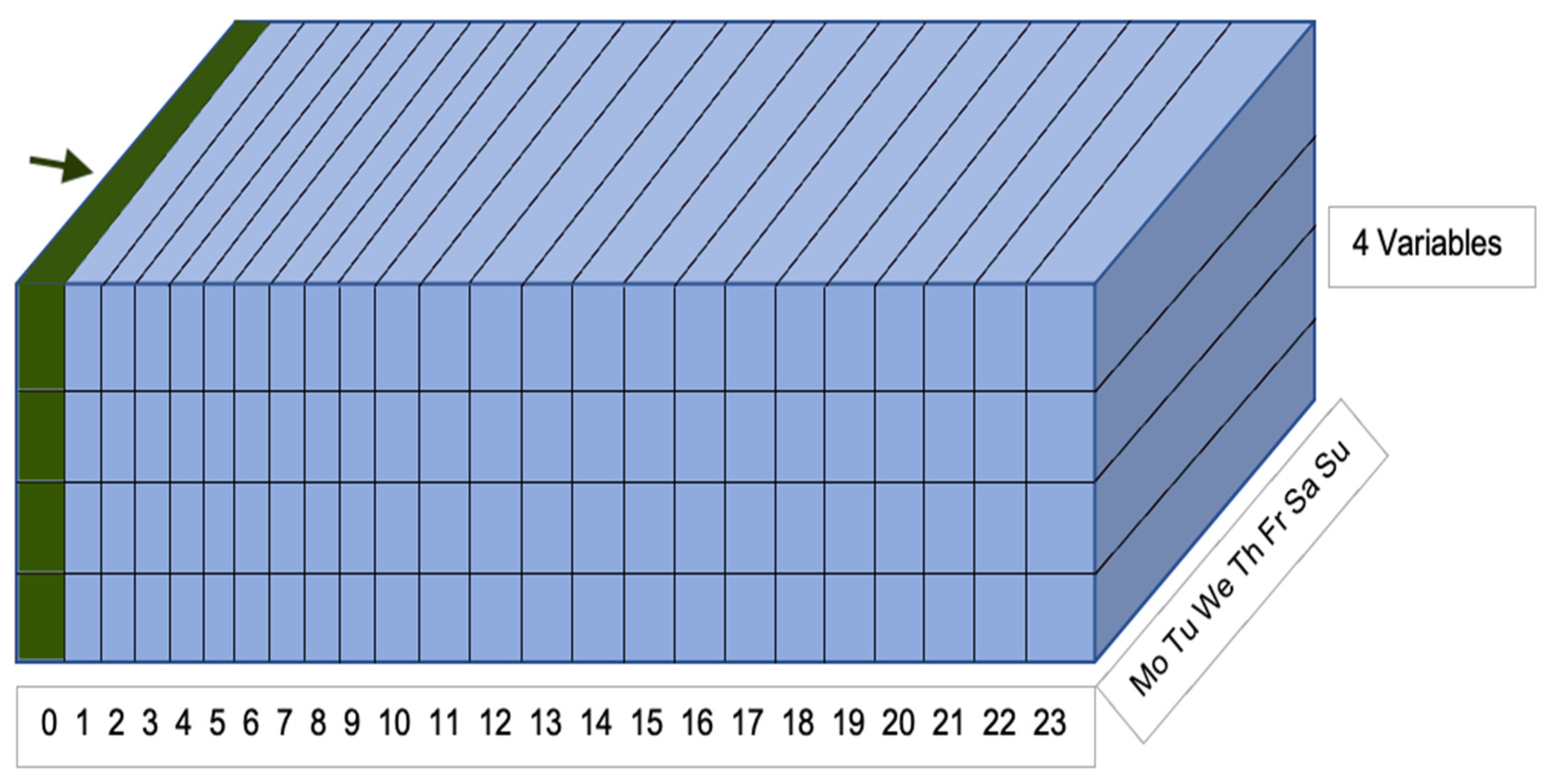
3.2.3. Used Variables

A multivariate time series analysis was utilised and the importance of the variables was tested. The CNN was initially run with all 18 variables for 300 epochs to establish the average validation MSE in the last ten epochs, which was taken as the control value. Following this, one variable in the model was set to the constant value of one and the model was rerun and the validation MSE was recorded. In each subsequent model run, a different variable was set to one each time. For each of these runs, the percentage difference to the control value was calculated. If this difference is positive, it highlights that the CNN performs better with this variable as a non-constant value and thus it is important, alternatively the variable can be removed.

Table 7. Variables utilised in CNN.

	Variables	Description	Unit of Measurement	Average % Difference to Control Value
1	Hourly power usage	Mean power usage per hour per customer, where: power = current × voltage	Wh	N.A.
2	Mean power	Mean weekly power values over the entire training period	Wh	1.059%
3	Days until month end	The number of days until the end of the month	Integer	0.926%
4	Province	Province in which the SHS is installed. Categories: Eastern, Southern, Western, Northern, Kigali City	Text	0.744%
5	Number of torches	Number of torches per customer	Integer	0.433%
6	Age	Customer age	Integer	0.405%
7	Number of bulbs	Number of bulbs per customer	Integer	0.337%
8	Maximum power	Maximum weekly power values over the entire training period	Wh	0.336%
9	Temperature	Hourly temperature recorded per SHS, i.e., customer	Celsius	0.346%
10	Number of TVs	Number of televisions per customer	Integer	0.340%
11	How heard about Bboxx	Method through which customer first heard about Bboxx. Categories: sales agent, flyer, other client, radio, shop, tv, other	Text	0.325%
12	Days from month start	The number of days from the start of the month	Integer	0.307%
13	Number of radios	Number of radios per customer	Integer	0.147%
14	Previous lighting source	Previous light or energy source used by customer. Categories: candles, batteries, lantern, other	Text	0.001%

displays the positive variables that were included in the CNN, with the first variable consisting of hourly power usage, which remained unaltered.

The most important variable according to the CNN was the mean hourly consumption over the previous four weeks. The second key variable concerned the number of days until the end of the month, indicating that customers’ usage differs across the month, potentially being related to when they receive their pay checks. This was followed by the province in which the customer resided, where a breakdown of energy consumption by province did highlight key differences in usage.

In addition to ensuring the variables were relevant, the researchers needed to choose the hyperparameter values, as discussed in Section 3.2.1. Different hyperparameter values were trialled on the validation dataset to test model performance. To aid the selection of hyperparameter values, Bayesian optimisation was used. Minimum and maximum values are chosen for each hyperparameter and the Bayesian optimiser starts off with a random value between these two to try on the validation dataset. The MAE is evaluated for each model run, where the optimiser is able to recall the values that performed well and can thus narrow down the range within the set number of model runs until it finds the optimal value [51]. In this study, the optimiser trialled 20 variants for each hyperparameter, where the CNN’s epoch number was 200, before the value with the lowest MAE was picked. Bayesian optimisation was used to determine multiple hyperparameter values, including dropout, number of input neurons and batch normalisation momentum, where the minimum and maximum ranges specified and the value eventually used for each are shown in

Table 8. Minimum to maximum hyperparameter values specified for Bayesian optimisation and the hyperparameter value used in presented CNN.

Hyperparameter	Min to Max Value Range	Value Used
Batch size	128–256	256
Dropout	0–0.7	0.5
Input neurons	128–2048	900
Batch normalisation momentum	0.6–0.99	0.65
Learning rate start Learning rate patience Learning rate weight decay Learning rate minimum	0.01–0.05 3–5 1 × 10−5–1 × 10−3 0.0005–0.002	0.02 5 1 × 10−4 0.001

.

An epoch number of 400 was used for all three forecasting scenarios. To reduce the likelihood of overfitting, the dropout method was utilised, where a specified number of neurons are arbitrarily deactivated. The validation loss continued to reduce during each model run, providing reassurance that overfitting did not occur.

4. Results and Discussion

4.1. Yearly Usage

The electricity consumption trends of SHS customers were observed at different timescales, including yearly, daily and hourly. Figure 4 shows the seven-day rolling mean for the year 2019 across all television and non-television owners.

The consumption is quite stable for customers without a television, whilst television owners experience more fluctuations (Figure 4). The variations in usage can stem from differences in weather conditions across the year, as was observed by Khan et al. [53]. Figure 4 also shows that SHS customers’ daily electricity consumption is relatively low. This is partly due to the SHS provider’s appliances being particularly energy efficient, in order to maximise SHS usage time. Soltowski et al. [54] found Rwandan users with 50 W SHS to have daily consumption levels up to 110 Wh, depending on the appliances owned. van der Plas and Hankins [55] observed an average daily energy usage of 113 Wh in Kenya. However, consumption can be even higher with a larger SHS capacity, where Heeten et al. [56] observed an average usage of 310 Wh per day when examining households with a 100 W SHS in Cambodia. Electricity consumption is constrained by the SHS capacity and the number of appliances owned and their efficiency. However, these results show that, on average, customers are far from reaching the capacity limit and many customers may find that smaller SHSs could sufficiently meet their needs. Previous studies have also observed that SHS users tend produce surplus energy [11,54].

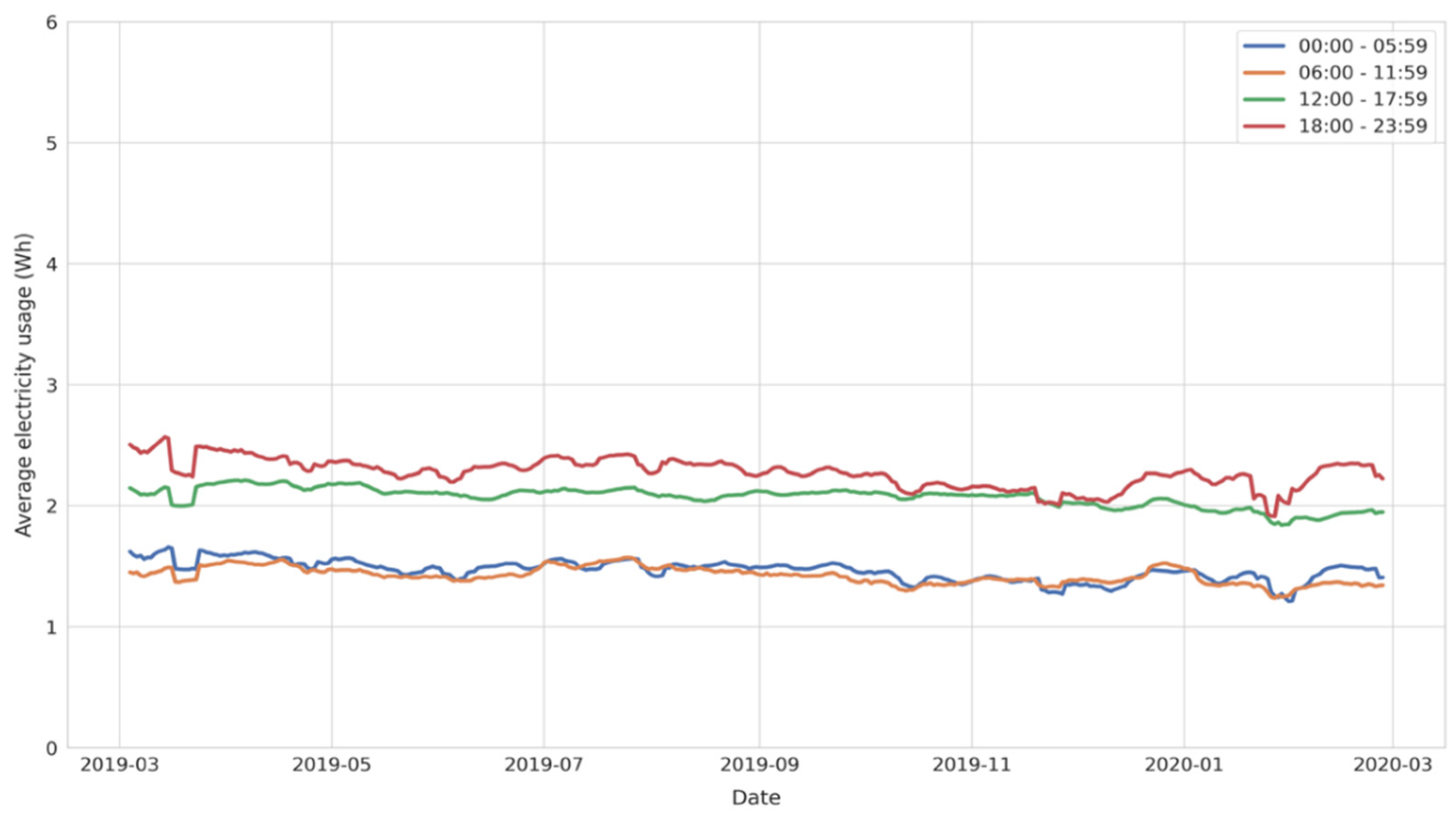
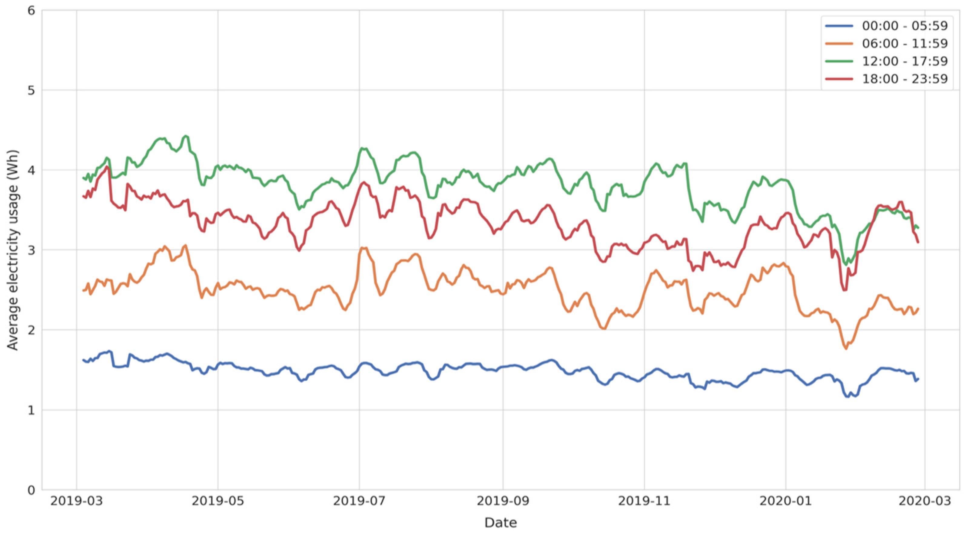
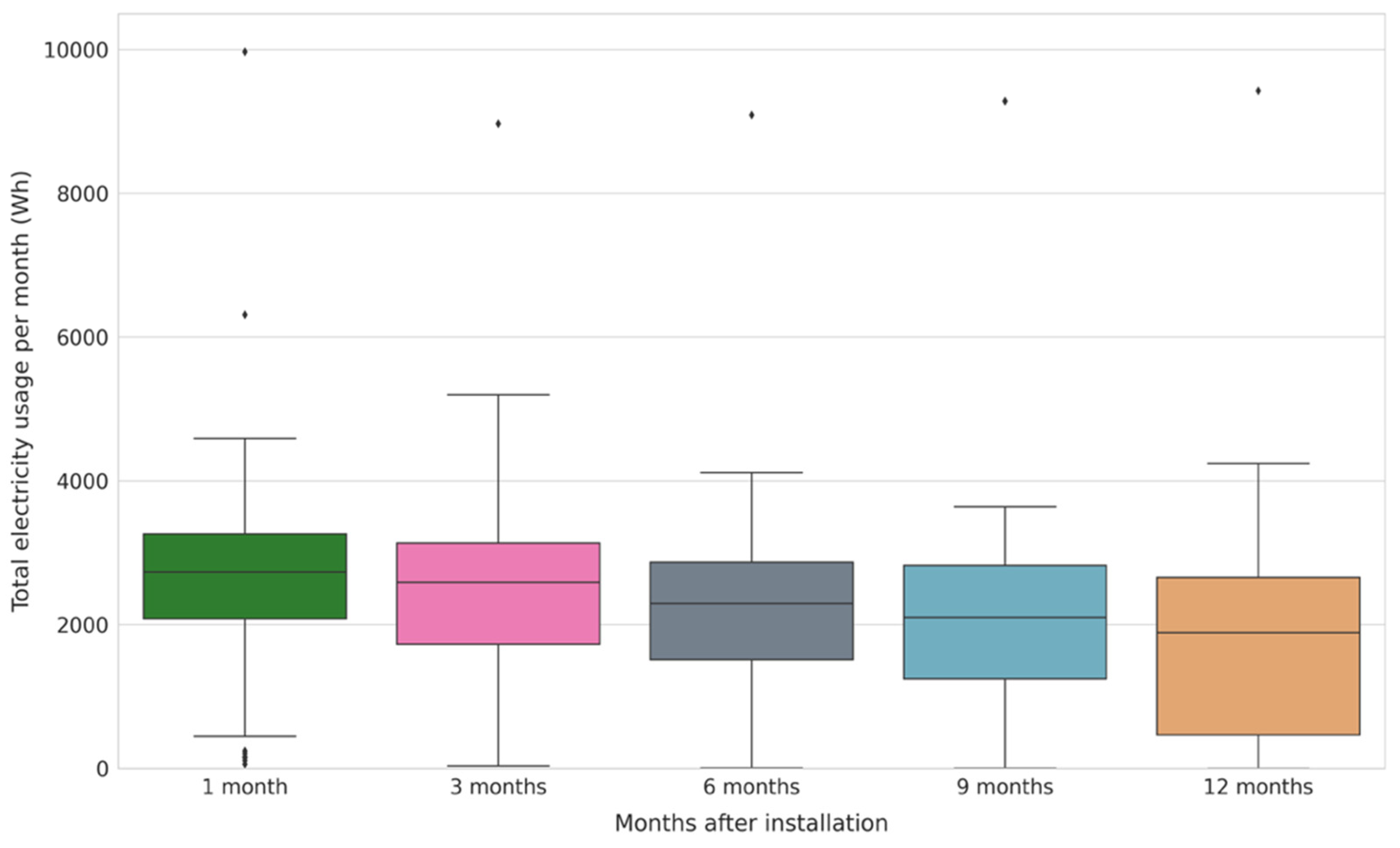
4.2. Usage across a Year

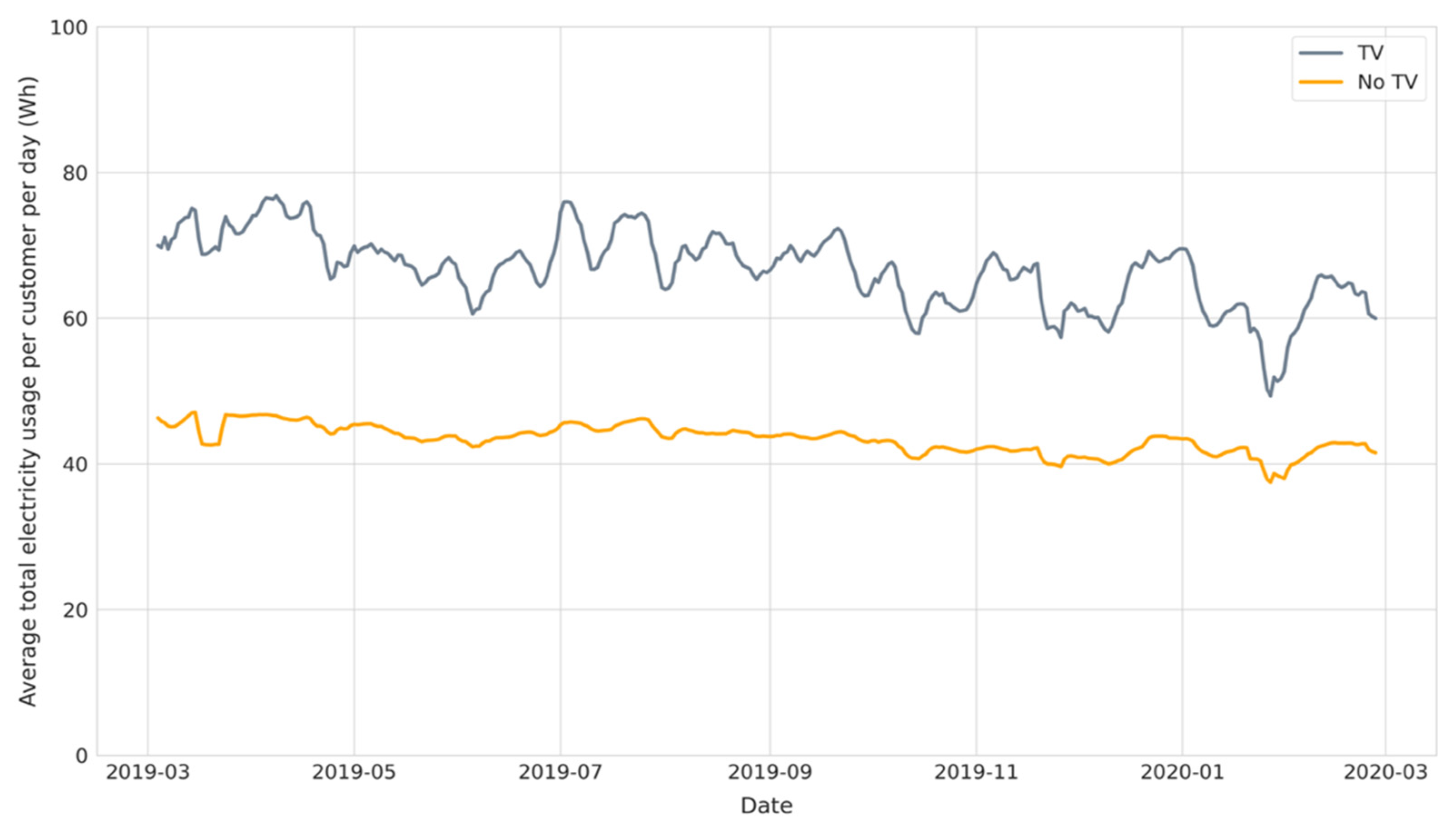
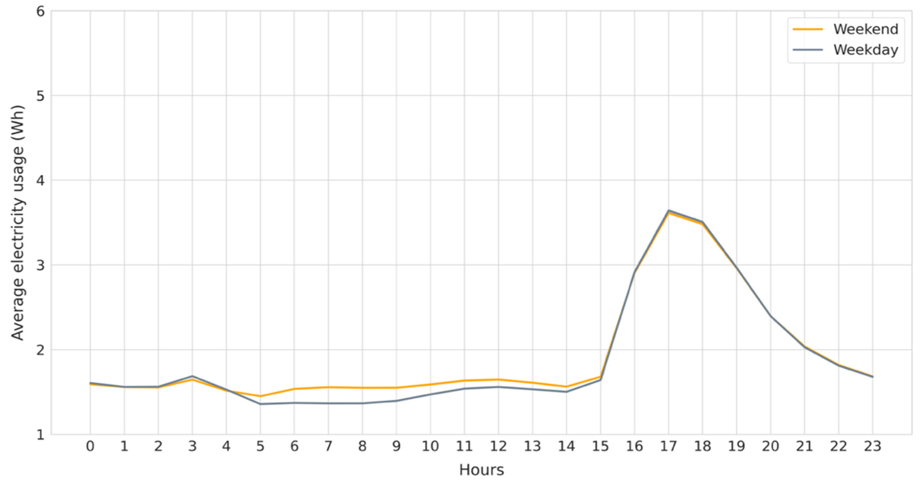
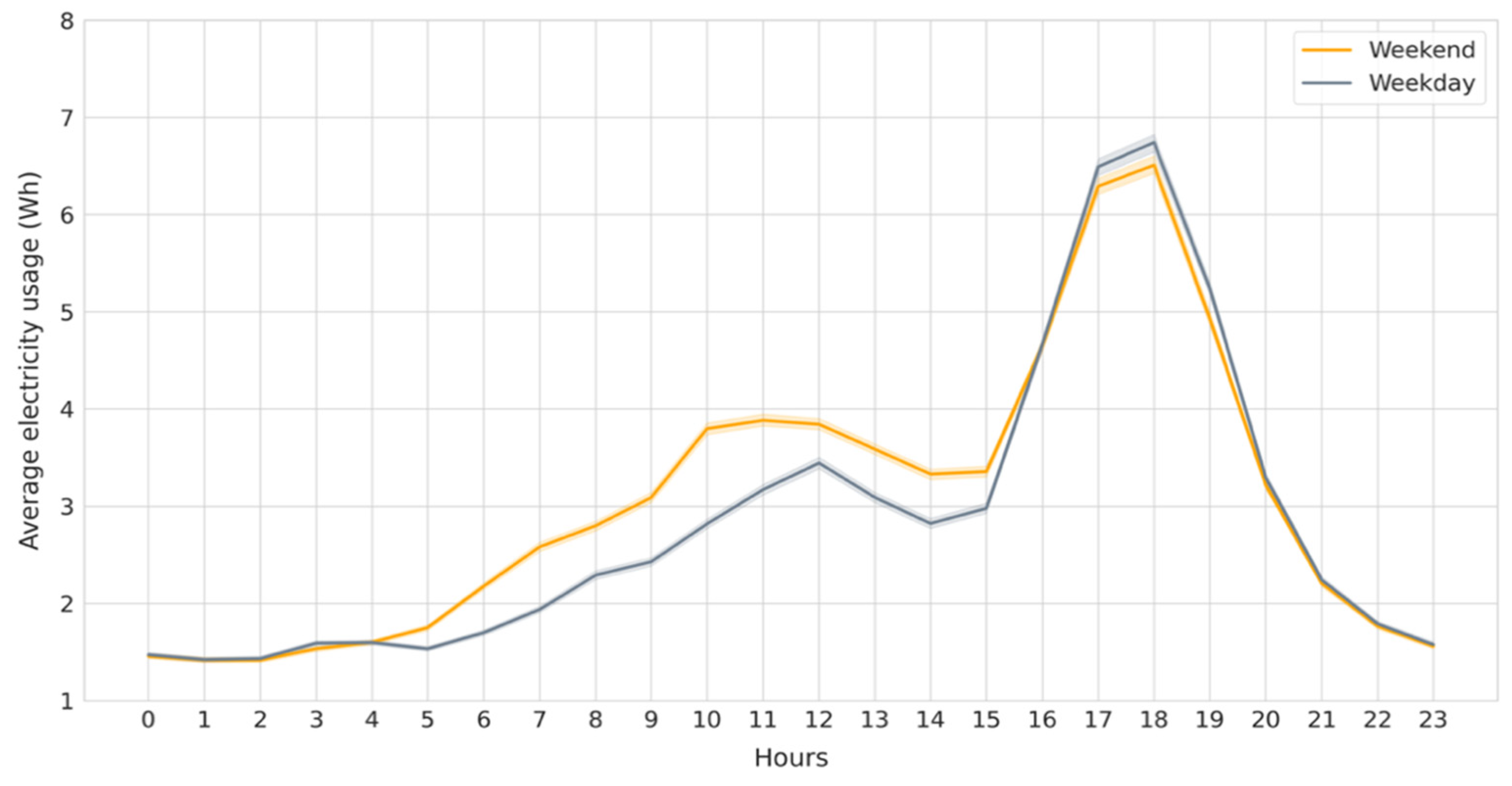
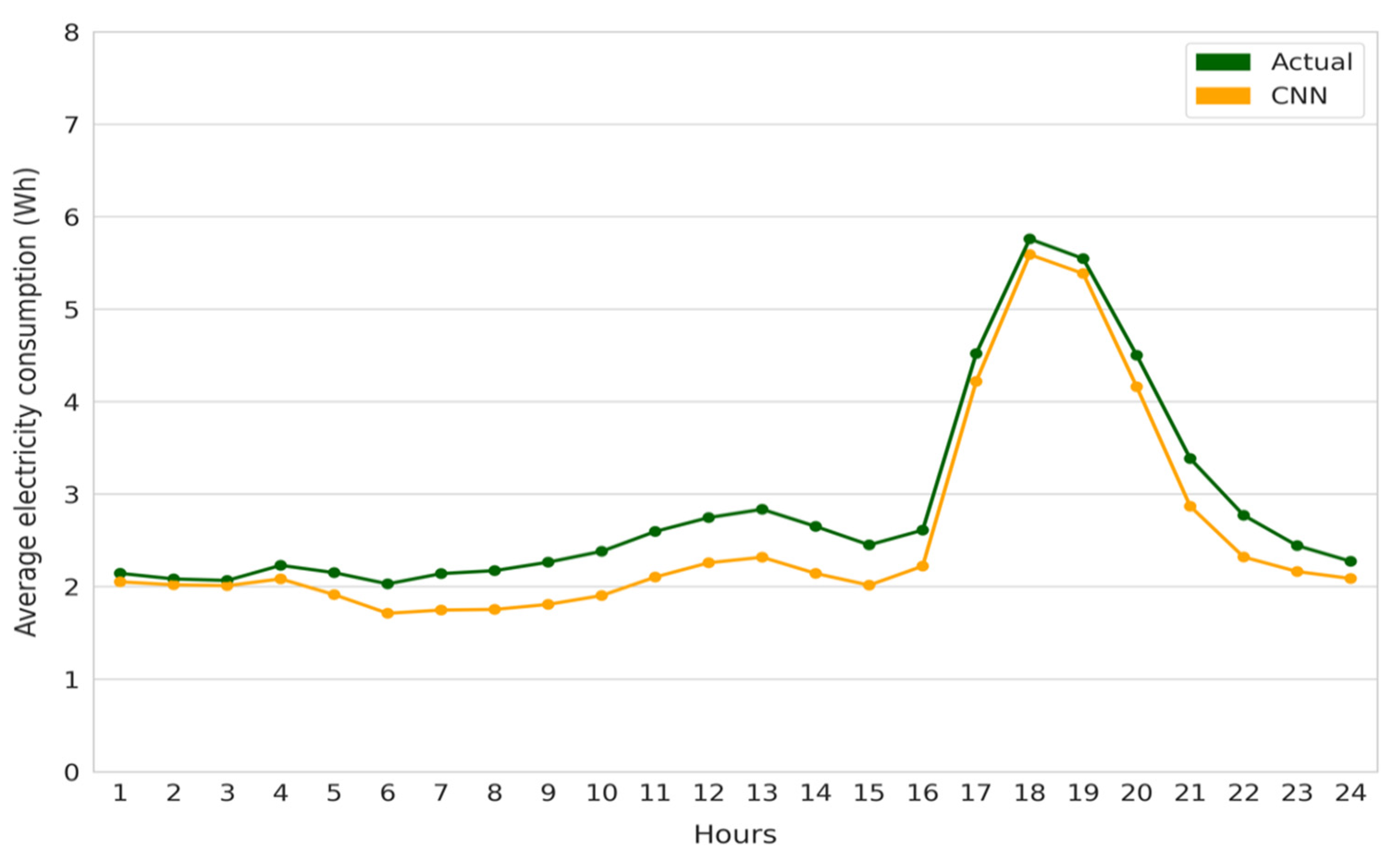
Households’ average electricity usage was split into four hourly groups to understand how consumption differs across time periods (Figure 5 and Figure 6).

Figure 5 and Figure 6 highlight that television owners mostly used their electricity in the afternoon (12:00–17:59) and evening, respectively, whilst customers without televisions saw the reverse pattern, using a large amount of electricity in the evening (18:00–23:59). The other key difference between the groups was that television owners used their SHS more in the morning period (06:00–11:59) compared to households that did not possess a television. This could be due to household occupants watching television at that time. Consumption at night was low and similar between television owners and households without a television. Gustavsson [8] examined Zambian SHS customers’ usage through data loggers and also found night-time usage to be low, particularly compared to the high consumption in the evening and morning. Although, the SHS usage did vary depending on appliance ownership, where high users’ peaks were particularly pronounced.

4.3. Daily Usage

Differences between weekday and weekend consumption were examined, where weekend usage was slightly higher (Figure 7 and Figure 8). However, this was only statistically significant for customers without a television (Wilcoxon Signed-Rank Test, p-value: 0.037).

Households’ electricity consumption may be higher at the weekend (Figure 7), due to more occupants being present in the house and additional usage of appliances [57,58]. Laicane et al. [59] also discovered that electricity usage was higher on the weekend, reasoning that families spent more time in the house than on weekdays. Figure 7 and Figure 8 highlight the hourly profile across a day, showcasing an evening peak from 17:00 to 18:00. Several studies observed that electricity grid users in both developing and developed countries faced a peak in usage in the evening. Soares and Medeiros [60] found peak hours to be between 19:00 and 21:00 for electricity consumers in Brazil. In Nigeria, grid users in rural areas experienced their evening peak between 17:00 and 22:00 [57]. Heeten et al. [56] observed a pronounced evening peak between 19:00 and 21:00 when examining 111 SHS customers in Cambodia. The increased usage in the evening is likely linked to a higher occupancy rate and fading daylight, the latter leading to lights being turned on.

Television customers in this study also experienced a second smaller usage peak in the afternoon between 11:00–13:00 (Figure 8). This could be linked to consumers watching television at that time, as households without a television do not have a comparable peak. This highlights a key distinction in behaviour between households with different appliances. Heeten et al. [56] also observed a usage peak around noon and suggested that it was due to the powering of a fan at lunchtime. McLoughlin et al. [61] used unsupervised clustering methods on residential electricity load data in Ireland to identify ten electricity load profiles depending on their customer characteristics. They discovered that each of these profiles had different load peaks, although most had a peak around midday [61]. This study offers a rare glimpse into SHS users’ daily usage patterns, with differences in consumption occurring based on whether it is a weekend and the appliance type owned. This knowledge enables SHS companies to provide a more targeted service that can better meet consumers’ needs.

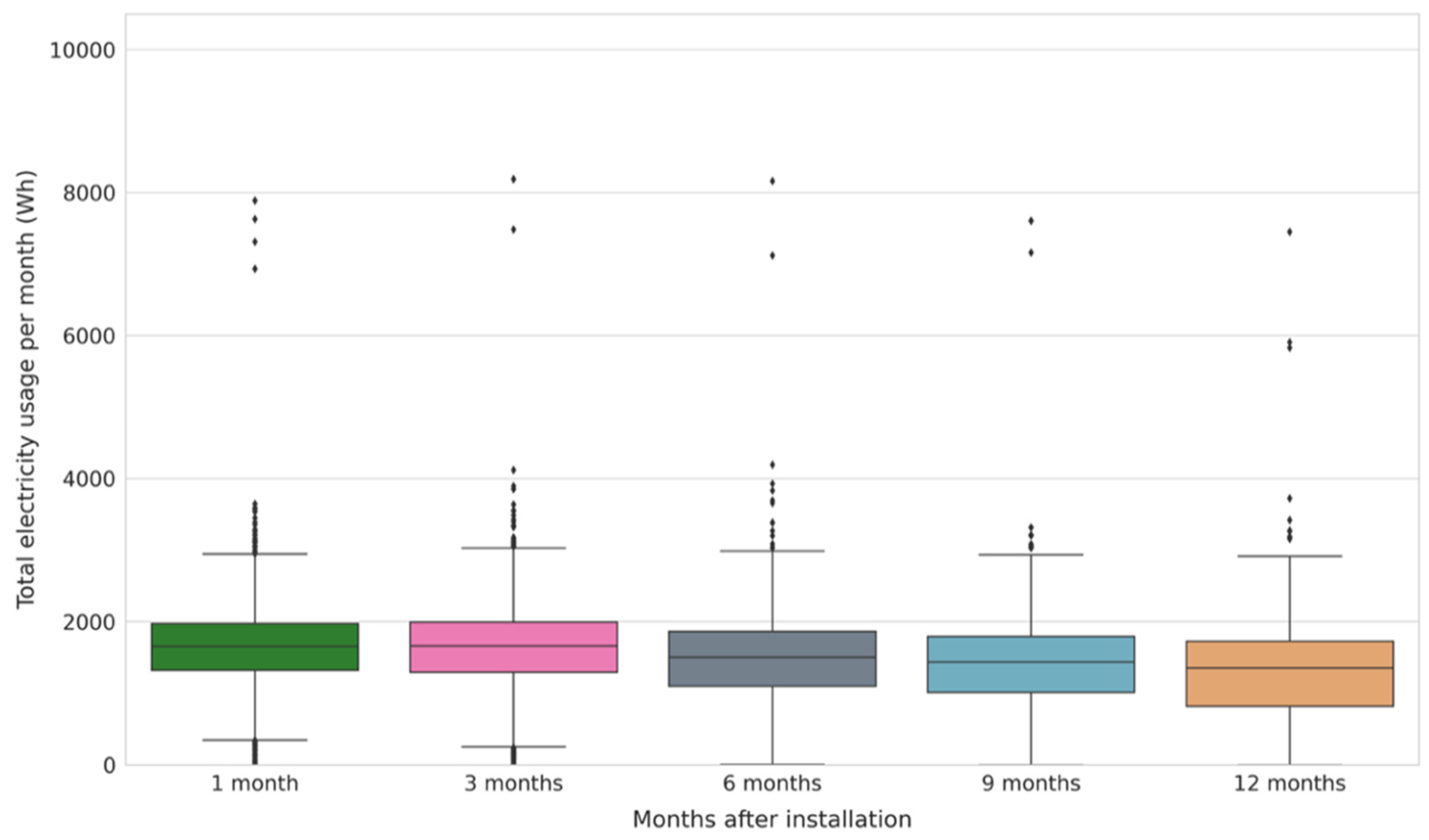
4.4. Usage Change per Customer

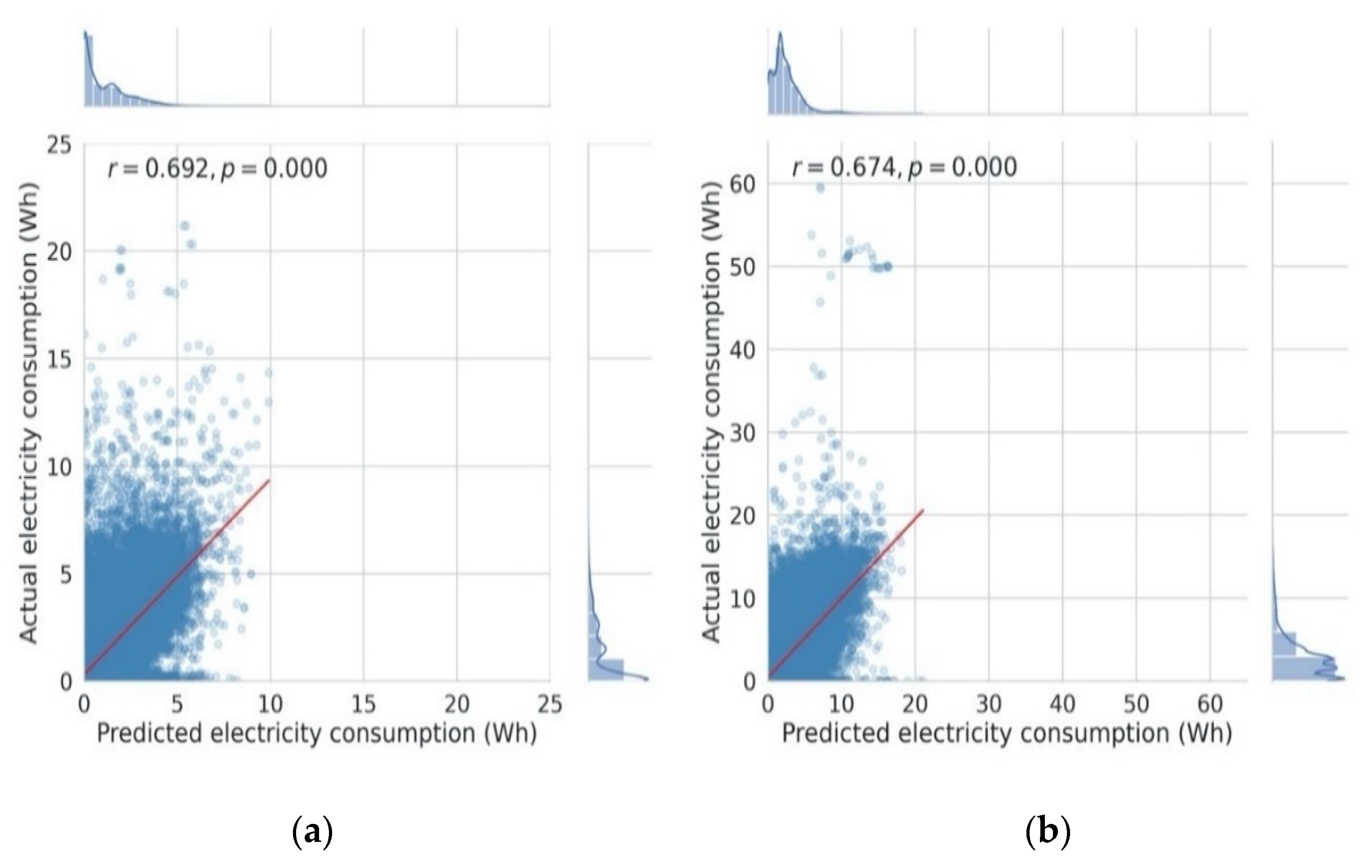
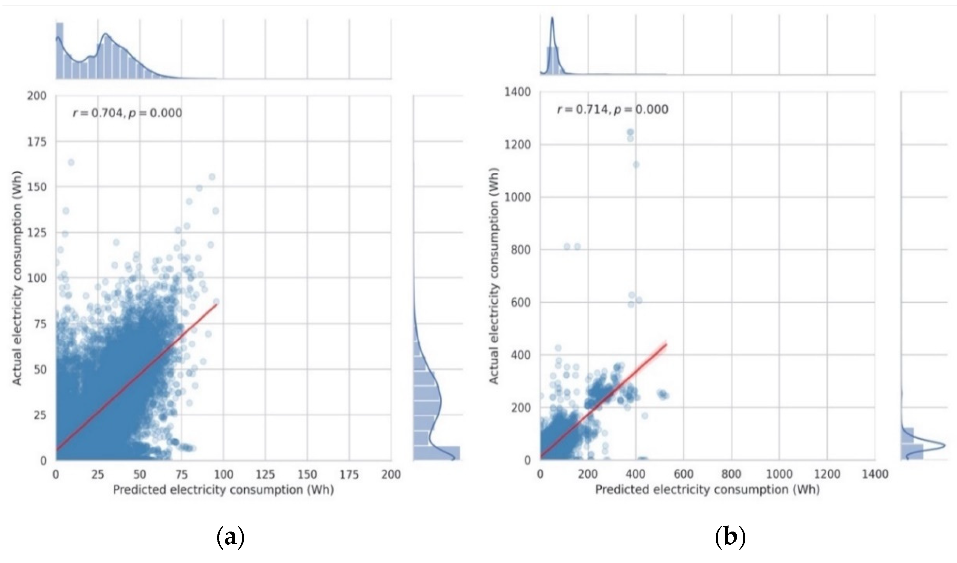
Another area of investigation covered whether and how SHS usage changes for individual consumers following their SHS installation. Households that became active customers between February and March 2019 and either owned a television or not were examined. Their total electricity usage in the month following installation, as well as six, nine and twelve months following this first month were recorded (Figure 9 and Figure 10).

The results highlight that television and non-television owners experienced a fall in usage after the first month (Figure 9 and Figure 10). This drop is especially evident for television customers (Figure 10). The t-test for paired samples performed reveals that for customers without a television the difference in households’ first month of electricity usage compared to a year later was statistically significant (t(2287) = 25.21, p-value = 5.82 × 10⁻¹²⁴). The difference between these two periods was also statistically significant for television owners (t(2287) = 9.70, p-value = 1.018 × 10⁻¹⁸). Specifically, 71% of non-television and 76% of television owners’ electricity usage decreased in a years’ time. The difference between each of the other intervals (3, 6, 9 months) and the first month of usage was also statistically significant. Customers with a television pay higher prices each month, which could thus leave them more vulnerable if their finances worsen after SHS purchase, leading to usage changes. SHS customers’ monthly income can be quite unstable and they may struggle to make electricity payments in particular months [62]. Television usage would also have a larger drain on a SHS’ battery compared to other appliances, which could deteriorate the battery’s performance and in due time affect consumption levels.

Few studies examined the question of whether SHS consumption rises over time. Opiyo [45] saw an increase in average daily electricity consumption for 27 Kenyan SHS users over a five-year period, which was accompanied by higher appliance ownership. However, this study utilised self-reported data on average daily usage, which might not be entirely accurate. Bisaga and Parikh [10] found that consumption did not increase across a three-month period of hourly data derived directly from the SHS. Although, in this short time, any alterations in usage may not have manifested themselves yet.

4.5. CNN Results

The 3D CNN was used to forecast three scenarios: 24 h ahead, daily sum for the next week and an average week across the next three months for low and higher energy users. The MSE for the CNN and naïve baseline forecasts are displayed in

Table 9. CNN and naïve baseline results for each scenario for low and high energy users (presented in an hourly format).

Scenario	Forecast Interval	Type of Energy User	Baseline MSE	CNN MSE	Percentage Difference
1	24 h	Low	2.788	1.386	50.3%
		High	8.052	4.577	43.2%
2	1 week (sum per day)	Low	0.669 (385) 1	0.382 (220) 1	42.9%
		High	2.014 (1160) 1	1.265 (729) 1	37.2%
3	3 months (hourly mean)	Low	0.768	0.369	52.0%
		High	2.568	1.194	53.5%

¹ Converted to daily format.

, which showcase their prediction performance for both types of energy users.

The results highlight that the CNN’s best performance compared to the naïve baseline was forecasting an average week across the next three months for both low and high energy users. The percentage difference between the CNN and baseline MSE was lowest in the second scenario, which forecasts the following week, although the CNN forecast was still superior.

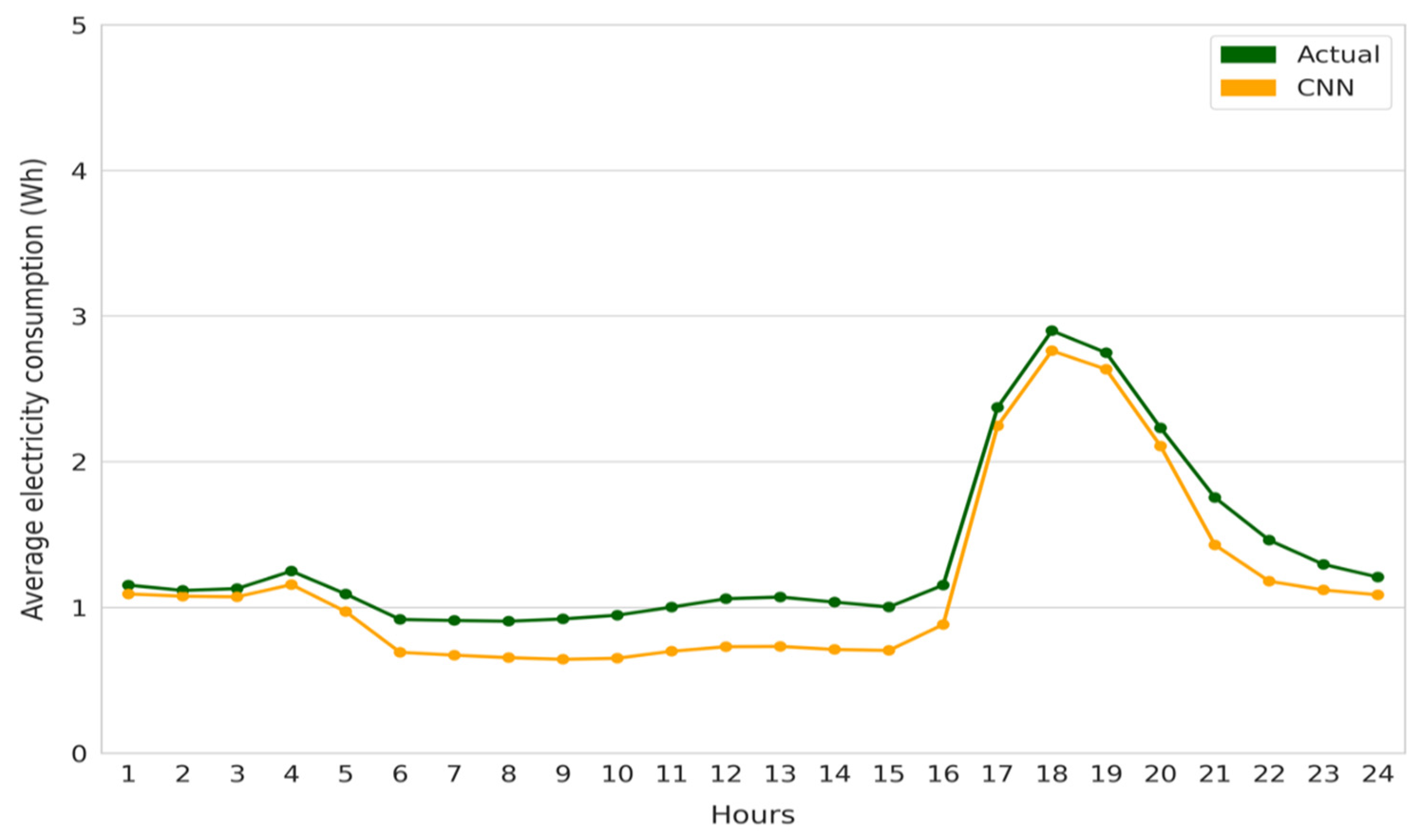
4.5.1. Scenario 1: 24 Hours

The first scenario consisted of the next 24 h of each individual households’ electricity usage. The CNN’s predictions compared to the actual hourly electricity consumption values for both low and high energy users are depicted in Figure 11. The Pearson correlation coefficient assesses the linear association between the CNN’s forecasted and actual values, where 1 represents perfect correlation [63]. In this case, the correlation coefficient was 0.692 and 0.674 for the low and high energy users, respectively (Figure 11a,b). Figure 11a,b show that actual hourly electricity consumption tends to be higher than the CNN predictions.

In the absence of SHS specific electricity load forecasting models, SHS operators likely rely on naïve baselines. In this scenario, the CNN performed over 40% better than such a naïve baseline for both low and high energy users (Table 9). As the CNN forecasts individual customers, it is difficult to portray the results representatively. Therefore, the average hourly electricity consumption over all test dataset customers was examined for low and high energy users, respectively (Figure 12 and Figure 13).

The results highlight that overall the CNN tends to predict lower values than SHS users’ actual consumption. The predictions are particularly close to reality in the morning hours and during the evening peak (Figure 12 and Figure 13). Gustavsson [8] also showed that households mainly utilised their SHS in the evening (18:00–21:00). The 24 h ahead forecast could be used by operators of SHS based microgrids to improve their ability to balance loads and anticipate potential demand surges. Soltowski et al. [54] highlights that connecting multiple SHSs to each other in such a microgrid would likely lead to less generated electricity being squandered.

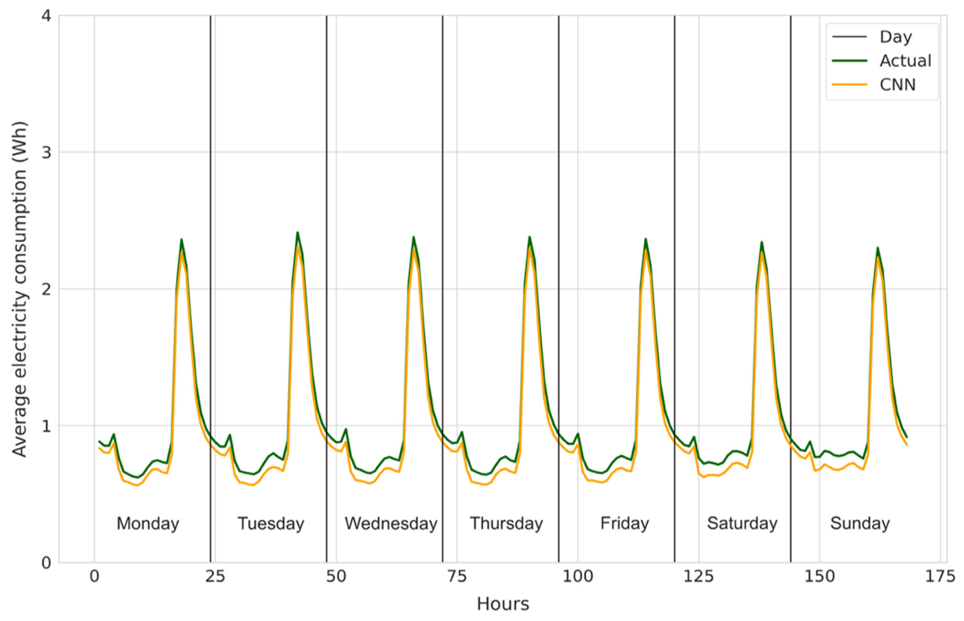
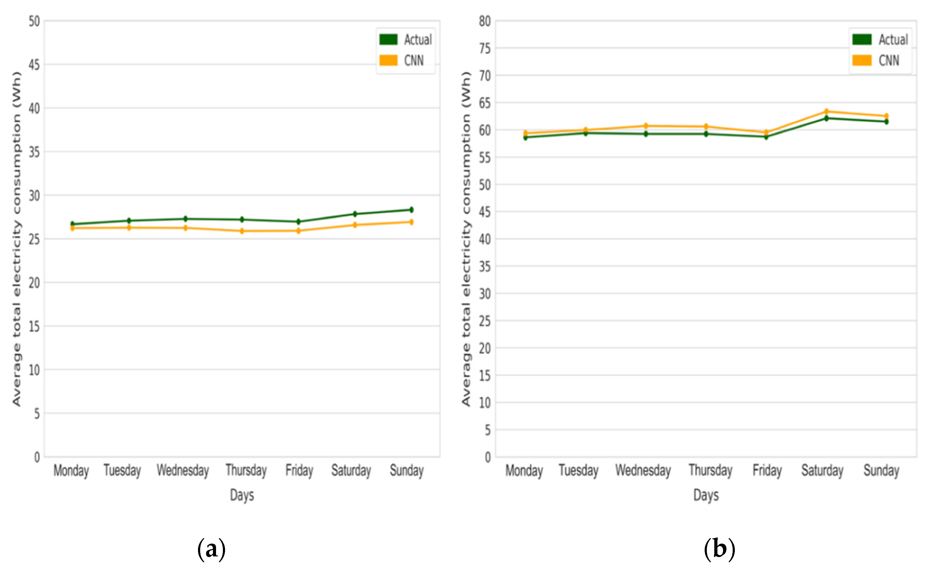
4.5.2. Scenario 2: 7 Daily Sums

The CNN forecasted the next seven days’ total daily electricity consumption for individual customers (Figure 14a,b). The low and high energy users had Pearson correlation coefficients of 0.704 and 0.714, respectively. Figure 14 shows that the CNN tends to predict that households consume less than they actually do.

Figure 15 displays customers’ actual electricity consumption and the CNN’s prediction for both low and high energy users. It highlights that the CNN performs generally well when forecasting the actual sum values for the next seven days.

The average actual daily consumption across customers is relatively stable over the week, although for high energy users there does appear to be an increase in usage on the weekend in Figure 15. SHS companies could provide valuable feedback to households on their expected energy usage for the next seven days through phone calls or visits. For instance, if these forecasts highlight a stark difference in usage for particular days in the next week, customers could be informed of this early on. This enables households to change their behaviour and reduce their likelihood of running out of battery. Consumers may also be interested to know by how much their consumption varies on a weekday compared to a weekend and reflect for what activities they utilise their SHS. As discussed in Section 2, previous studies highlighted the effectiveness of such feedback interventions on changing consumption behaviour [16,39]. Both Fischer [64] and Karjalainen [65] observed that households value regular feedback information on their past electricity usage. Moreover, consumers could be informed of their likely future electricity usage based on the model’s forecast, enabling them to manage their upcoming expenditure [41,42]. Future studies could trial this approach to gauge the impact on households’ electricity consumption and perceived financial control.

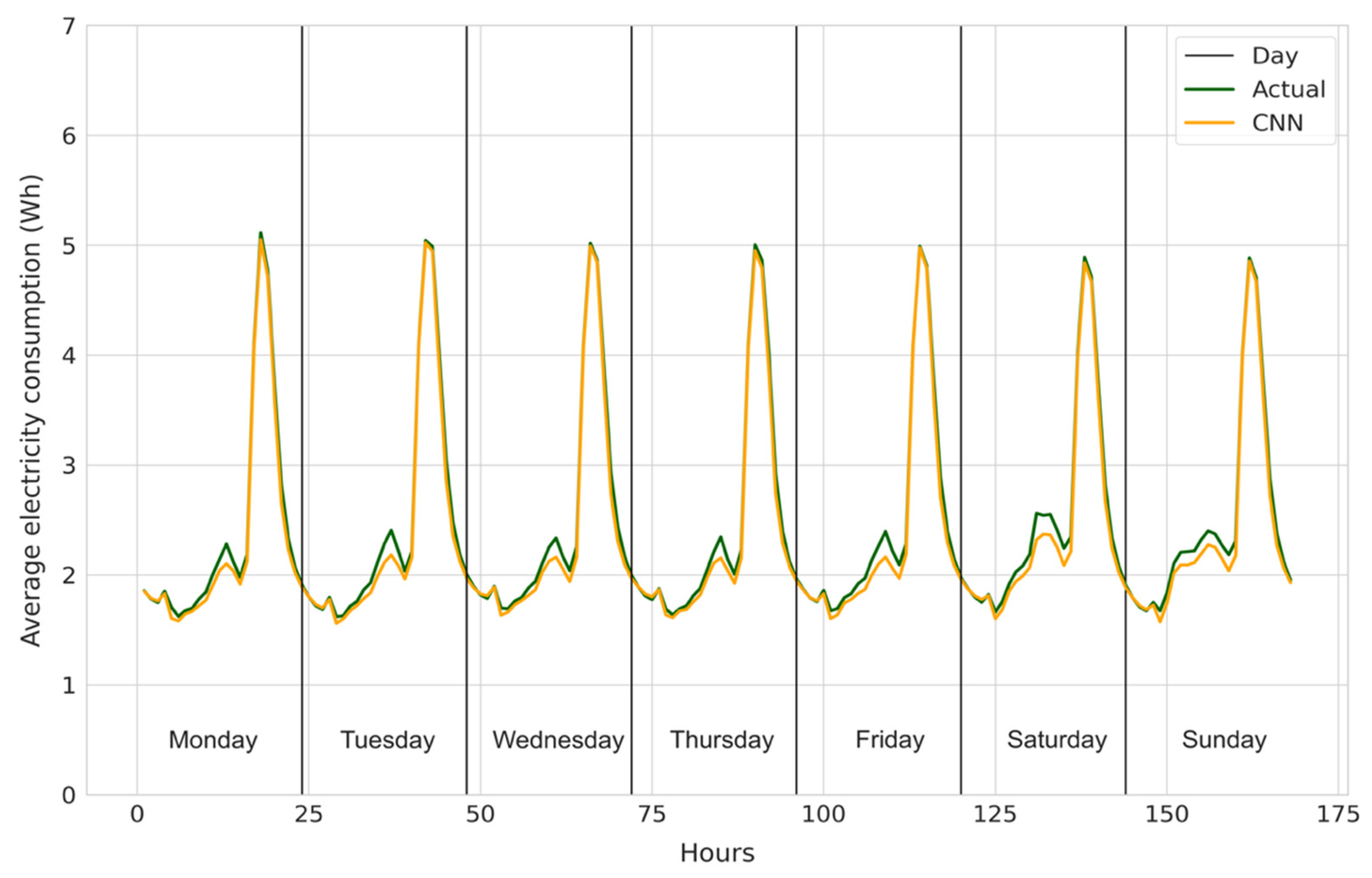
4.5.3. Scenario 3: Usage across 3 Months

The final scenario consists of forecasting an average week in the next three months for each customer. This prediction offers a more robust picture of a household’s future consumption than if the CNN was tasked with only predicting a week 3 months in the future, which may feature atypical usage patterns. This scenario shows households’ average usage in the future, enabling decisions based on these forecasts to be made more confidently. The CNN performs better in this average based scenario compared to forecasting sum values (Figure 16a,b). The Pearson correlation coefficients for low and high energy users are 0.795 and 0.811, respectively. The CNN is more likely to predict higher usage values compared to the actual values in the high energy scenario, which accounts for the outliers in Figure 16b.

The electricity consumption of all low and high energy consumers within the test dataset are pictured in Figure 17 and Figure 18, respectively. The CNN’s forecasted results nearly match the real values, although the model tends to be quite cautious, being prone to predict lower peaks than actually occurred.

The electricity consumption across a week for the whole customer base is relatively stable and follows a regular pattern (Figure 17 and Figure 18). High energy users had a more pronounced peak during midday compared to low energy users. A similar distinction was observed in the behaviour of television and non-television owners in Section 4.3, with television owners also experiencing this midday peak.

The SHS provider can use these predictions to better cater to their customers’ needs based on their specific past and future usage profile. For instance, a household’s forecast may reveal that their consumption levels will result in them regularly running out of battery, which other studies have also identified as an issue affecting consumers [8,12]. The company could then intervene by giving customers the option to switch to a SHS with a higher capacity that would match their requirements. Policymakers could also aggregate these load forecasts to a district or even province level to pinpoint areas that will experience high average consumption levels. This information, in addition to an investigation of the districts’ past usage trends, could factor into decision-making on where future microgrids should be built or grid expansion should commence. Zeyringer et al. [66] highlighted the importance of regionally specific electricity planning, as in certain areas decentralised solar solutions can be more cost efficient than grid expansion.

5. Conclusions

Significant strides were made to increase energy access over recent years, including providing additional support for off-grid energy technologies, which have grown in prominence. However, more work is urgently required to achieve energy access for all by 2030. To aid this mission, it is important to gain a better insight of the households that adopt off-grid energy systems, such as SHSs, to understand both how they use them and for what purpose. This enables off-grid energy providers to reach unelectrified households more effectively and retain customers that are at risk of repossession.

This paper provided a rare insight into SHS customers’ electricity usage based on a large-scale analysis of real-time data derived directly from the SHSs of 63,299 households. The past usage trends revealed differences in daily electricity consumption patterns for television owners and those without a television. In addition to an evening peak, television owners also experienced a second usage peak in the afternoon. This study found that for over 70% of customers monthly electricity consumption had decreased a year after SHS installation. This highlights that merely owning a SHS is not enough, as households also require the financial stability to make regular payments in the long run. SHS providers and policymakers should take note of this finding and examine possible strategies to aid affordability. These could include companies offering longer payment periods or the government introducing end-user subsidies.

This is the first study to utilise a CNN to forecast SHS customers’ electricity consumption and one of the first to use a 3D CNN architecture for load forecasting with time series data, as far as the authors are aware. A novel 3D CNN was tested on three scenarios, which forecasted individual SHS customers’ electricity consumption. These consisted of predicting 24 h ahead, the daily sum for the next week and an average week across the next three months for low and high energy users. The CNN’s performance was consistently superior when predicting low energy users compared to high energy users’ consumption and the lowest MSE was derived when forecasting an average week across the next three months. This study highlights the value of using an advanced forecasting model, such as a 3D CNN, which outperformed the naïve baseline in each scenario. Despite the challenge of SHS users’ highly variable electricity usage, this study argues that more electricity forecasting should be performed, as the results could aid policymakers, off-grid energy providers and households. SHS companies could use these predictions to offer a more tailored service to individual households and provide them with direct feedback, enabling customers to better budget for their future expenditure and avoid running out of battery. The CNN could also be utilised to aid load balancing for SHS based microgrids and help policymakers to identify areas with high consumption that could be well-placed for future grid expansion.

The findings of this research and the developed model could be applied to a multitude of contexts. It would be insightful if future studies used this type of model to forecast individual household’s consumption in different countries to observe potential similarities or differences. To gain an even deeper insight of customers’ usage pattens, more advanced clustering techniques should be considered. Different models could be used to forecast SHS users’ future electricity consumption, including a LSTM or a one-dimensional CNN, whose performance could then be compared to this study’s CNN. Finally, future studies could test the performance of 3D CNNs for other load forecasting purposes.

References

1. IEA Access to Electricity Database, Electronic Dataset, IEA, Paris. 2020. Available online: https://www.iea.org/reports/sdg7-data-and-projections/access-to-electricity (accessed on 19 June 2021).
2. United Nations The Sustainable Development Goals Report 2016; United Nations Publications: New York, NY, USA, 2016.
3. Zerriffi, H. Innovative business models for the scale-up of energy access efforts for the poorest. Curr. Opin. Environ. Sustain. 2011, 3, 272–278. [Google Scholar] [CrossRef]
4. Lighting Global; GOGLA; ESMAP. Off-Grid Solar Market Trends Report 2020; Lighting Global Program: Washington, DC, USA, 2020. [Google Scholar]
5. Narayan, N.; Chamseddine, A.; Vega-Garita, V.; Qin, Z.; Popovic-Gerber, J.; Bauer, P.; Zeman, M. Exploring the boundaries of Solar Home Systems (SHS) for off-grid electrification: Optimal SHS sizing for the multi-tier framework for household electricity access. Appl. Energy 2019, 240, 907–917. [Google Scholar] [CrossRef]
6. Koo, B.B.; Rysankova, D.; Portale, E.; Angelou, N.; Keller, S.; Padam, G. Rwanda: Beyond Connections; World Bank: Washington, DC, USA, 2018. [Google Scholar]
7. IEA Africa Energy Outlook 2019; IEA Publications: Paris, France, 2019.
8. Gustavsson, M. With time comes increased loads—An analysis of solar home system use in Lundazi, Zambia. Renew. Energy 2007, 32, 796–813. [Google Scholar] [CrossRef]
9. Opoku, R.; Obeng, G.Y.; Adjei, E.A.; Davis, F.; Akuffo, F.O. Integrated system efficiency in reducing redundancy and promoting residential renewable energy in countries without net-metering: A case study of a SHS in Ghana. Renew. Energy 2020, 155, 65–78. [Google Scholar] [CrossRef]
10. Bisaga, I.; Parikh, P. To climb or not to climb? Investigating energy use behaviour among Solar Home System adopters through energy ladder and social practice lens. Energy Res. Soc. Sci. 2018, 44, 293–303. [Google Scholar] [CrossRef] [Green Version]
11. Bhatti, S.; Williams, A. Estimation of surplus energy in off-grid solar home systems. Renew. Energy Environ. Sustain. 2021, 6, 25. [Google Scholar] [CrossRef]
12. Manur, A.; Marathe, M.; Manur, A.; Ramachandra, A.; Subbarao, S.; Venkataramanan, G. Smart Solar Home System with Solar Forecasting. Proceedings of 2020 IEEE International Conference on Power Electronics, Smart Grid and Renewable Energy (PESGRE2020), Cochin, India, 2–4 January 2020; pp. 1–6. [Google Scholar] [CrossRef]
13. Andersen, F.M.; Larsen, H.V.; Boomsma, T.K. Long-term forecasting of hourly electricity load: Identification of consumption profiles and segmentation of customers. Energy Convers. Manag. 2013, 68, 244–252. [Google Scholar] [CrossRef]
14. Aung, Z.; Toukhy, M.; Williams, J.R.; Sanchez, A.; Herrero, S. Towards Accurate Electricity Load Forecasting in Smart Grids. In Proceedings of the DBKDA 2012: The Fourth International Conference on Advances in Databases, Knowledge, and Data Applications, Reunion Island, France, 1 March 2012; IARIA: Saint Gilles, Brussels, 2012. [Google Scholar]
15. Humeau, S.; Wijaya, T.K.; Vasirani, M.; Aberer, K. Electricity load forecasting for residential customers: Exploiting aggregation and correlation between households. In Proceedings of the 2013 Sustainable Internet and ICT for Sustainability SustainIT, Palermo, Italy, 30–31 October 2013; pp. 1–6. [Google Scholar] [CrossRef] [Green Version]
16. Schultz, P.W.; Estrada, M.; Schmitt, J.; Sokoloski, R.; Silva-Send, N. Using in-home displays to provide smart meter feedback about household electricity consumption: A randomized control trial comparing kilowatts, cost, and social norms. Energy 2015, 90, 351–358. [Google Scholar] [CrossRef] [Green Version]
17. Gajowniczek, K.; Zabkowski, T. Short term electricity forecasting using individual smart meter data. Procedia Comput. Sci. 2014, 35, 589–597. [Google Scholar] [CrossRef] [Green Version]
18. Efficiency for Access Coalition. The State of the Off-Grid Appliance Market; Efficiency for Access Coalition, 2019. [Google Scholar]
19. Practical Action. Poor People’s Energy Outlook 2014; Practical Action Publishing: Rugby, UK, 2014. [Google Scholar]
20. Wang, Q.; Li, S.; Li, R. Forecasting energy demand in China and India: Using single-linear, hybrid-linear, and non-linear time series forecast techniques. Energy 2018, 161, 821–831. [Google Scholar] [CrossRef]
21. Kuster, C.; Rezgui, Y.; Mourshed, M. Electrical load forecasting models: A critical systematic review. Sustain. Cities Soc. 2017, 35, 257–270. [Google Scholar] [CrossRef]
22. Lazzeri, F. Machine Learning for Time Series Forecasting with Python; John Wiley & Sons, Inc.: Indianapolis, Indiana, 2020. [Google Scholar]
23. Dostál, P. Forecasting of Time Series with Fuzzy Logic. In Prediction, Modeling and Analysis of Complex Systems. Advances in Intelligent Systems and Computing; Zelinka, I., Chen, G., Rössler, O., Snasel, V.A.A., Eds.; Springer: Berlin/Heidelberg, Germany, 2013. [Google Scholar]
24. González, P.A.; Zamarreño, J.M. Prediction of hourly energy consumption in buildings based on a feedback artificial neural network. Energy Build. 2005, 37, 595–601. [Google Scholar] [CrossRef]
25. Nielsen, M.A. A visual proof that neural nets can compute any function. In Neural Networks and Deep Learning; Determination Press: San Francisco, CA, USA, 2015. [Google Scholar]
26. Pujari, P.; Sewak, M.; Rezaul Karim, M. Practical Convolutional Neural Networks; Packt Publishing: Birmingham, UK, 2018; ISBN 978-1-78839-230-3. [Google Scholar]
27. Amran, N.A.; Soltani, M.D.; Yaghoobi, M.; Safari, M. Deep Learning Based Signal Detection for OFDM VLC Systems. In Proceedings of the 2020 IEEE International Conference on Communications Workshops (ICC Workshops), Online, 7–10 June 2020; pp. 1–6. [Google Scholar]
28. Acharya, S.K.; Wi, Y.M.; Lee, J. Short-term load forecasting for a single household based on convolution neural networks using data augmentation. Energies 2019, 12, 3560. [Google Scholar] [CrossRef] [Green Version]
29. Amarasinghe, K.; Marino, D.L.; Manic, M. Deep neural networks for energy load forecasting. In Proceedings of the 2017 IEEE 26th International Symposium on Industrial Electronics (ISIE), Edinburgh, UK, 19–21 June 2017; pp. 1483–1488. [Google Scholar] [CrossRef]
30. Lang, C.; Steinborn, F.; Steffens, O.; Lang, E.W. Electricity load forecasting—An evaluation of simple 1D-CNN network structures. arXiv 2019, arXiv:1911.11536. [Google Scholar]
31. Koprinska, I.; Wu, D.; Wang, Z. Convolutional Neural Networks for Energy Time Series Forecasting. In Proceedings of the 2018 International Joint Conference on Neural Networks (IJCNN), Rio de Janeiro, Brazil, 8–13 July 2018; pp. 1–8. [Google Scholar] [CrossRef]
32. Heo, J.; Song, K.; Han, S.; Lee, D.-E. Multi-channel convolutional neural network for integration of meteorological and geographical features in solar power forecasting. Appl. Energy 2021, 295, 1–13. [Google Scholar] [CrossRef]
33. Kiguchi, Y.; Heo, Y.; Weeks, M.; Choudhary, R. Predicting intra-day load profiles under time-of-use tariffs using smart meter data. Energy 2019, 173, 959–970. [Google Scholar] [CrossRef]
34. Mack, B.; Tampe-Mai, K.; Kouros, J.; Roth, F.; Taube, O.; Diesch, E. Bridging the electricity saving intention-behavior gap: A German field experiment with a smart meter website. Energy Res. Soc. Sci. 2019, 53, 34–46. [Google Scholar] [CrossRef]
35. Komatsu, H.; Kimura, O. Peak demand alert system based on electricity demand forecasting for smart meter data. Energy Build. 2020, 225, 1–14. [Google Scholar] [CrossRef]
36. Guo, Z.; Zhou, K.; Zhang, C.; Lu, X.; Chen, W.; Yang, S. Residential electricity consumption behavior: Influencing factors, related theories and intervention strategies. Renew. Sustain. Energy Rev. 2018, 81, 399–412. [Google Scholar] [CrossRef]
37. Bonan, J.; Adda, G.; Mahmud, M.; Said, F. The Role of Flexibility and Planning in Repayment Discipline: Evidence from a Field Experiment on Pay-as-You-Go Off-Grid Electricity; Working Paper: Milan, Italy, 2020. [Google Scholar]
38. Zhang, X.M.; Grolinger, K.; Capretz, M.A.M.; Seewald, L. Forecasting Residential Energy Consumption: Single Household Perspective. In Proceedings of the 2018 17th IEEE International Conference on Machine Learning and Applications (ICMLA), Orlando, FL, USA, 17–20 December 2018; pp. 110–117. [Google Scholar] [CrossRef]
39. Gans, W.; Alberini, A.; Longo, A. Smart meter devices and the effect of feedback on residential electricity consumption: Evidence from a natural experiment in Northern Ireland. Energy Econ. 2013, 36, 729–743. [Google Scholar] [CrossRef] [Green Version]
40. Dominicis, S. De; Sokoloski, R.; Jaeger, C.M.; Schultz, P.W. Making the smart meter social promotes long-term energy conservation. Palgrave Commun. 2019, 5, 1–8. [Google Scholar] [CrossRef] [Green Version]
41. Gajowniczek, K.; Ząbkowski, T. Electricity forecasting on the individual household level enhanced based on activity patterns. PLoS One 2017, 12, 1–26. [Google Scholar] [CrossRef] [PubMed] [Green Version]
42. Chen, C.; Cook, D.J. Behavior-Based Home Energy Prediction. In Proceedings of the 2012 Eighth International Conference on Intelligent Environments (IE ’12), Guanajuato, Mexico, 26–29 June 2012; IEEE Computer Society: Washington, DC, USA, 2012; pp. 57–63. [Google Scholar]
43. Chitsaz, H.; Shaker, H.; Zareipour, H.; Wood, D.; Amjady, N. Short-term electricity load forecasting of buildings in microgrids. Energy Build. 2015, 99, 50–60. [Google Scholar] [CrossRef]
44. Kizilcec, V.; Parikh, P. Solar Home Systems: A comprehensive literature review for Sub-Saharan Africa. Energy Sustain. Dev. 2020, 58, 78–89. [Google Scholar] [CrossRef]
45. Opiyo, N.N. How basic access to electricity stimulates temporally increasing load demands by households in rural developing communities. Energy Sustain. Dev. 2020, 59, 97–106. [Google Scholar] [CrossRef]
46. Bisaga, I.; Puźniak-Holford, N.; Grealish, A.; Baker-Brian, C.; Parikh, P. Scalable off-grid energy services enabled by IoT: A case study of BBOXX SMART Solar. Energy Policy 2017, 109, 199–207. [Google Scholar] [CrossRef] [Green Version]
47. Abdul-Salam, Y.; Phimister, E. Modelling the impact of market imperfections on farm household investment in stand-alone solar PV systems. World Dev. 2019, 116, 66–76. [Google Scholar] [CrossRef]
48. Adwek, G.; Boxiong, S.; Ndolo, P.O.; Siagi, Z.O.; Chepsaigutt, C.; Kemunto, C.M.; Arowo, M.; Shimmon, J.; Simiyu, P.; Yabo, A.C. The solar energy access in Kenya: A review focusing on Pay-As-You-Go solar home system. Env. Dev Sustain. 2019, 22, 3897–3938. [Google Scholar] [CrossRef]
49. Lay, J.; Ondraczek, J.; Stoever, J. Renewables in the energy transition: Evidence on solar home systems and lighting fuel choice in Kenya. Energy Econ. 2013, 40, 350–359. [Google Scholar] [CrossRef] [Green Version]
50. Witten, I.H.; Frank, E.; Hall, M.A.; Pal, C.J. Data Mining, 4th ed.; Morgan Kaufmann: Cambridge, MA, USA, 2017; ISBN 978-0-12-804291-5. [Google Scholar]
51. Agrawal, T. Hyperparameter Optimization in Machine Learning: Make Your Machine Learning and Deep Learning Models More Efficient; Apress Standard: New York, NY, USA, 2021; ISBN 978-1-4842-6578-9. [Google Scholar]
52. Hyndman, R.J.; Athanasopoulos, G. Forecasting: Principles and Practice, 2nd ed.; OTexts: Melbourne, Australia, 2018. [Google Scholar]
53. Khan, S.I.; Raihan, S.A.; Habibullah, M.; Abrar, S.F. Reducing the cost of solar home system using the data from data logger. In Proceedings of the 2017 IEEE International Conference on Smart Grid and Smart Cities (ICSGSC), Singapore, 23–26 July 2017; pp. 37–41. [Google Scholar]
54. Soltowski, B.; Bowes, J.; Strachan, S.; Anaya-Lara, O.L. A Simulation-Based Evaluation of the Benefits and Barriers to Interconnected Solar Home Systems in East Africa. In Proceedings of the 2018 IEEE PES/IAS PowerAfrica, Cape Town, South Africa, 28–29 June 2018; pp. 491–496. [Google Scholar] [CrossRef] [Green Version]
55. van der Plas, R.J.; Hankins, M. Solar electricity in Africa: A reality. Energy Policy 1998, 26, 295–305. [Google Scholar] [CrossRef]
56. Heeten, T. Den; Narayan, N.; Diehl, J.; Verschelling, J.; Silvester, S.; Popovic-Gerber, J.; Bauer, P.; Zeman, M. Understanding the present and the future electricity needs: Consequences for design of future Solar Home Systems for off-grid rural electrification. In Proceedings of the 2017 International Conference on the Domestic Use of Energy (DUE), Cape Town, South Africa, 4–5 April 2017; pp. 8–15. [Google Scholar]
57. Adeoye, O.; Spataru, C. Modelling and forecasting hourly electricity demand in West African countries. Appl. Energy 2019, 242, 311–333. [Google Scholar] [CrossRef]
58. Marszal-Pomianowska, A.; Heiselberg, P.; Larsen, O.K. Household electricity demand profiles—A high-resolution load model to facilitate modelling of energy flexible buildings. Energy 2016, 103, 487–501. [Google Scholar] [CrossRef]
59. Laicane, I.; Blumberga, D.; Blumberga, A.; Rosa, M. Evaluation of Household Electricity Savings. Analysis of Household Electricity Demand Profile and User Activities. Energy Procedia 2015, 72, 285–292. [Google Scholar] [CrossRef] [Green Version]
60. Soares, L.J.; Medeiros, M.C. Modeling and forecasting short-term electricity load: A comparison of methods with an application to Brazilian data. Int. J. Forecast. 2008, 24, 630–644. [Google Scholar] [CrossRef]
61. McLoughlin, F.; Duffy, A.; Conlon, M. A clustering approach to domestic electricity load profile characterisation using smart metering data. Appl. Energy 2015, 141, 190–199. [Google Scholar] [CrossRef] [Green Version]
62. Kizilcec, V.; Parikh, P.; Bisaga, I. Examining the Journey of a Pay-as-You-Go Solar Home System Customer: A Case Study of Rwanda. Energies 2021, 14, 330. [Google Scholar] [CrossRef]
63. Sedgwick, P. Pearson’s correlation coefficient. BMJ 2012, 345, 1. [Google Scholar] [CrossRef] [Green Version]
64. Fischer, C. Feedback on household electricity consumption: A tool for saving energy? Energy Effic. 2008, 1, 79–104. [Google Scholar] [CrossRef]
65. Karjalainen, S. Consumer preferences for feedback on household electricity consumption. Energy Build. 2011, 43, 458–467. [Google Scholar] [CrossRef]
66. Zeyringer, M.; Pachauri, S.; Schmid, E.; Schmidt, J.; Worrell, E.; Morawetz, U.B. Analyzing grid extension and stand-alone photovoltaic systems for the cost-effective electrification of Kenya. Energy Sustain. Dev. 2015, 25, 75–86. [Google Scholar] [CrossRef]
Figure 1. Flow chart of the steps involved in the model development process.
Energies 15 00857 g001
Figure 2. CNN architecture.
Energies 15 00857 g002
Figure 3. Used 3D CNN data structure for ‘weekly view’ (stacked by hours, days, variables). Arrow indicates first data slice examined.
Energies 15 00857 g003
Figure 4. Average total electricity usage per customer per day for both television and non-television owners (7-day rolling mean).
Energies 15 00857 g004
Figure 5. Average total electricity usage per customer per day for non-television owners (7-day rolling mean).
Energies 15 00857 g005
Figure 6. Average electricity usage by hour groups across a year for television owners (7-day rolling mean).
Energies 15 00857 g006
Figure 7. Weekday and weekend hourly average electricity usage for non-television owners.
Energies 15 00857 g007
Figure 8. Weekday and weekend hourly average electricity usage for television owners.
Energies 15 00857 g008
Figure 9. Box plots of the total electricity usage per month for non-television owners after installation (n = 2288). Box shows the interquartile range from 25th to 75th percentile, the outer horizontal lines (whiskers) refer to the 10th and 90th percentile and the dots represent outliers.
Energies 15 00857 g009
Figure 10. Box plot of the total electricity usage per month for television owners after installation (n = 219). Box shows the interquartile range from 25th to 75th percentile, the outer horizontal lines (whiskers) refer to the 10th and 90th percentile and the dots represent outliers.
Energies 15 00857 g010
Figure 11. Actual hourly electricity usage versus CNN’s hourly prediction for the next 24 h: (a) Low energy users; (b): High energy users.
Energies 15 00857 g011
Figure 12. Average electricity usage over all test dataset customers for the next 24 h. Figure shows actual values and CNN forecast for low energy users.
Energies 15 00857 g012
Figure 13. Average electricity usage over all test dataset customers for the next 24 h. Figure shows actual values and CNN forecast for high energy users.
Energies 15 00857 g013
Figure 14. Actual electricity usage versus CNN’s prediction for 7 daily sums: (a): Low energy users; (b): High energy users.
Energies 15 00857 g014
Figure 15. Average over all test dataset customers for next week’s daily sums. Figure shows actual values and CNN forecast: (a): Low energy users; (b): High energy users.
Energies 15 00857 g015
Figure 16. Scatter plot of actual electricity usage versus CNN’s prediction for a week over next three months: (a): Low energy users; (b): High energy users.
Energies 15 00857 g016
Figure 17. CNN forecast versus the actual average electricity usage of a week over next three months for all low energy test dataset customers. The black vertical line separates the days.
Energies 15 00857 g017
Figure 18. CNN forecast versus the actual average electricity usage of a week over next three months for all high energy test dataset customers. The black vertical line separates the days.
Energies 15 00857 g018