Prediction of Electric Buses Energy Consumption from Trip Parameters Using Deep Learning

Abstract

The energy demand of electric buses (EBs) is a very important parameter that should be considered by transport companies when introducing electric buses into the urban bus fleet. This article proposes a novel deep-learning-based model for predicting energy consumption of an electric bus traveling in an urban area. The model addresses two important issues: accuracy and cost of prediction. The aim of the research was to develop the deep-learning-based prediction model, which requires only the data readily available to bus fleet operators, such as location of the bus stops (coordinates, altitude), route traveled, schedule, travel time between stops, and to find the most suitable type and configuration of neural network to evaluate the model. The developed prediction model was assessed with different types of deep neural networks using real data collected for several bus lines in a medium-sized city in Poland. Conducted research has shown that the deep learning network with autoencoders (DLNA) neural network allows for the most accurate energy consumption estimation of 93%. The proposed model can be used by public transport companies to plan driving schedules and energy management when introducing electric buses.

1. Introduction

Public transport is critical to the operation of urban systems. Worldwide, more and more attention is being paid to reducing the environmental impact of transport. There is still a growing discussion on converting transport to so-called clean transport (using clean fuels) while improving service availability [1]. The popularity of electrification of public urban transport is growing due to the low greenhouse gas emissions and noise reduction compared to buses with conventional drive.

The electrification of existing bus fleets requires determining the electric bus range and methods of charging, as well as planning the charging infrastructure and schedule that will not interrupt normal bus operation. Designing an efficient electric bus network also requires determining the energy demand and selecting the appropriate battery capacity. The energy demand varies throughout the day under different traffic conditions which makes it difficult to estimate using conventional methods.

Efficient operation of electric buses requires a good charging planning strategy in daily operation, mainly due to the limited capacity of the batteries [2]. The complexity of the task is influenced by the number of public transport lines and the diversity of the bus fleet [3].

In the literature, there are studies in which the energy demand for electric buses was estimated by calculating the average demand for the distance traveled or travel time. The types of bus and travel conditions were not taken into account [4,5]. This approach is often used in studies related to the planning of charging electric buses. This approach is very simple to implement, but the use of average energy consumption values only gives a rough estimate of energy needs and does not take into account route features such as degree of inclination and travel conditions of travels at different times of the day. During peak hours, bus journeys can take much more time than off-peak hours (often over 50%), resulting in a much higher energy demand.

In this article, we propose a novel, original deep learning model for predicting energy consumption of a battery electric bus that uses readily available parameters: travel time between stops, the difference in altitude between stops, rush hours for a given line, weather conditions, and the distance between bus stops. The acquisition of such parameters does not introduce any additional excessive costs to bus operators and does not require specialized equipment or many additional person-hours. The model performs well with various types of networks and, even with regression function, achieves high accuracy of the prediction.

Selection of parameters, impacting the energy consumption of electric buses, is based on our statistical analysis of available real data. With such easily obtainable data, the developed model predicts energy consumption with 93% of accuracy.

The behavior and accuracy of any model depends also on the neural network type used to evaluate it. Thus, the aim of the research was also to find a neural network type and configuration which provides the best accuracy of the prediction. We have considered various configurations and types of neural networks, such as deep learning networks with an autoencoder layer (DLNA) and a network of long short-term memory (LSTM) type. For comparison, the model was also evaluated with a classic multilayer perceptron (MLP) network.

The work presented here is a continuation of the research from [6]. The work presented here aimed at improving the accuracy of the model without cost increase. Thorough analysis of available real data for additional bus lines showed that there are other parameters which can strongly impact the prediction accuracy. Our new energy demand prediction model includes a new input parameter—the peak hour. We describe how to enter this parameter in Section 3.

To evaluate the model, we considered other neural network types and their configurations, searching for the one which will provide the best results. Additionally, data from other bus lines was also analyzed and used to evaluate the model.

In the literature, there are many models for estimating energy consumption of electric buses based on artificial intelligence methods, but to the best of the authors’ knowledge, no model has been found that, based on similar parameters, would allow for estimating energy consumption with the accuracy that we have obtained in our research. Most models require specific input data not readily available, requiring additional measurements or complex measurement devices, which generates costs to bus operators.

Highlights of this work:

• A novel deep learning model for predicting energy consumption of battery electric buses in an urban area.
• The model uses five readily available bus travel parameters: travel time between stops, the difference in altitude between stops, rush hours for a given line, weather conditions, and the distance between bus stops; thus, it can be easily applied to any urban bus network, avoiding unnecessary expenses on additional specialized equipment.
• The model performs well with various types of neural networks.
• The model provides at least 93% accuracy of energy consumption estimate regardless of neural network used (validated on real data for several bus lines).
• The proposed model could bring benefits in energy-related transport planning and traffic operation studies.

The rest of the article is organized as follows. Section 2 reviews existing energy consumption models and neural network types and configurations used for their validation. Section 3 provides information on the dataset used for training, validation, and testing of the proposed model and more details on data analysis. At the end of the section, the methodology used to derive the model is presented. Section 4 presents the derived energy demand prediction model and discusses the architectures of the chosen deep learning neural networks on which the described model is evaluated. Section 5 presents the results of the experimental studies obtained with the proposed approach and discusses the results. Lastly, Section 6 contains conclusions and future research plans.

2. Energy Consumption Models and Neural Networks

A number of analytical models have been proposed in the literature to estimate energy consumption. For example, [7] presents a simplified model of estimating the energy demand of electric buses in the existing bus networks. The input data of the model consists of information about the arrival and departure times of buses. High-resolution bus journey profile information is not needed.

In other studies, standard driving cycles from literature data were used [8,9,10]. Driving cycle measurements are based on traffic measurements carried out in different cities. However, applying the standard driving cycle in a different city may lead to different results. Moreover, this study does not take into account the traffic conditions for different bus lines. They are usually not identical, especially on large bus networks, as buses have a low average speed with many stops and a long delay in reaching the stop.

The results of the studies presented in [11] indicate that an estimate of energy can be obtained using route characteristics, such as distance covered, inclination of the road and number of turns, and travel parameters, such as speed and acceleration. The presented case studies involve a small number of routes and indicate a need for further validation of the proposed estimation method.

The authors in [12] developed a general framework for estimating the energy demand of electric buses. After analyzing electric bus journeys using mapping data from the spatial information system for large bus networks, they noticed that the difference in height for the bus route is one of the main factors of energy consumption.

In [13], the authors investigated the influence of environmental conditions, route characteristics, and dynamic traffic conditions on the energy consumption of electric buses. The results showed that including more variables can significantly improve forecasting performance. The research described in this paper shows that route characteristics have the largest impact on energy consumption. This is important for journeys of less than 20 km. The conclusions of this study are consistent with the results obtained in our article. Compared to [6], which used four input parameters, the addition of the fifth parameter improved the accuracy of energy consumption estimation by one percentage point, from 7.2% to 6.2% (MAPE—mean absolute percentage error).

The energy consumption of electric buses (EBs) depends on various factors, such as vehicle characteristics, vehicle speed, road grade and acceleration, frequency of stops, weather conditions (air conditioning and heating), etc. [14]. In fact, these factors vary widely, making energy consumption estimation a complex problem. The study of [15] also found that topography and the frequency of stops have a large impact (9.5% and 8.3%, respectively) on the EB energy consumption.

Energy consumption models for EBs are very different to other electric vehicles (EV). In [16,17], the impact of the number of passengers getting on and off, as well as auxiliary systems, was studied. Such models usually require additional data that is difficult to obtain, e.g., the numbers of passengers getting on and off.

In [18,19], authors proposed a model based on explicit modeling of the motor efficiency. In particular, good performance was estimated from component-based simulations using vehicle-specific data provided by the manufacturer.

The nonlinearity and complexity caused by a combination of factors impacting energy consumption make the problem too complex for standard techniques but appropriate for a deep learning approach.

In recent literature, descriptions of many models for estimating energy consumption can be found, but there are few models that utilize deep learning and data that is readily available from bus fleet operators. The increase in computing power of personal computers (NVIDIA graphics cards, above 8 GB of RAM, fast SSD disks) and the improvement of learning algorithms made it possible to effectively train deep learning networks [20]. For this reason, deep learning architectures have found application in solving many problems, such as classification and recognition of images, forecasting traffic intensity, and predicting the result based on a sequence of parameters.

In [21], a probabilistic model of energy consumption using machine learning was proposed. The model makes it possible to estimate the energy consumption for road connections. The authors obtained an error in estimating their energy consumption less than 6%. However, the test data only covered a 4-day period in January, so it is not very representative. Parameters taken into account were state of charge, auxiliary power, and vehicle speed.

Another example of the use of deep learning to predict vehicle speed is presented in [22]. The speed prediction method is based on historical data such as vehicle speed, acceleration, location, and driving date. The authors state that the use of deep learning networks has produced satisfactory results.

The LSTM network was used for speed prediction in [23] and for estimating engine power [24]. The LSTM training is performed on the dataset collected from the traffic simulator using real data representing described city routes.

In [25], authors conducted an analysis of deep learning methods used in the energy sector. Deep learning was found to be very useful for problems related to new perspectives on energy, including state estimation, generation of renewable scenarios, and power grid synthesis. This article presents the energy demand model that does not require high-resolution velocity profile measurements or any other sophisticated data.

The development of electromobility in smart cities in Poland is an important research topic [26]. The case study was performed for data obtained from a public transport company (PKM Jaworzno) in the city of Jaworzno in Poland, which has been successfully introducing battery electric buses into its fleet for several years [27].

As a result of the analysis of the actual available data, we determined the impact of various bus travel parameters on energy consumption. To assess the demand for energy, we proposed to use five parameters, such as travel time between stops, the difference in altitude between stops, rush hours for a given line, weather conditions, and the distance between bus stops.

Although the preparation of the model requires a time-consuming and precise preparation of the training sequence as well as the selection of the type and appropriate configuration of the neural network, after training, such a model allows to quickly and accurately estimate the energy consumption of an existing system.

The thorough analysis of neural network types and configuration yields that the proposed model performs best with a deep learning neural network with autoencoders.

Such a model evaluated for a routes simulator can provide vital information to electric bus network infrastructure designers. It may be also useful for solving other electric bus fleet problems related to battery size, charging strategy, and infrastructure.

The presented work, by providing experimental results, proves that a deep learning architecture is suitable for the problem of energy estimation of EBs. Considering the promising results of the conducted experiments, we plan to evaluate other types of deep learning networks and its usability to a derived energy estimation model.

Key achievements of this work:

• A novel deep learning prediction model using readily available parameters increasing the accuracy of energy consumption estimation.
• Determination of parameters influencing the energy consumption of electric buses based on statistical analysis of available real data.
• Determination of the type and configuration of neural network which is best suited to implement and evaluate the model to provide the best accuracy.

3. Dataset Description, Analysis, and Methodology

The first step required to prepare a useful prediction model was to classify obtained datasets and thoroughly analyze them to determine all parameters which could strongly impact energy consumption of EBs.

3.1. Dataset

The data obtained from a public transport company PKM Jaworzno includes the GPS coordinates of the bus stops locations, the arrival times at bus stops, and the energy consumed between successive stops (state of battery on consecutive bus stops).

The aim of data analysis was to determine the impact of various available parameters on the energy consumption of an electric bus between consecutive bus stops.

Data were registered for working days in summer and winter months of 2018 (July, August, September excluded); one working day in each month, except for holiday months. Data were collected throughout the day from around 5 a.m. to 11 p.m. for two bus lines. As the bus line is, in many cases, a loop (buses travel the same routes cyclically), the data was recorded multiple times for the same round-trip connections. Due to this, it is possible to check the change of energy consumption of the bus introduced by the stops elevation, traffic density, and rush hours in different seasons and weather conditions. In total, energy consumption was analyzed for over 4000 journeys between 136 stops. Electric buses with batteries with a capacity of 160 kWh (Solaris Urbino 12 Electric) were taken into account.

Sample data for nine consecutive stops visited during the bus operation on one of the PKM Jaworzno bus lines (blue line in Figure 1) in February are presented in

Table 1. Bus journey parameters.

No.	Bus Stop Name	GPS Coordinates of Bus Stops		Time of Arrival	Energy Consumption (kWh)
1	SD	19.292681	50.246734	09:35:13	bsp 1
2	SPrz	19.294296	50.243577	09:36:13	0.50
3	SOG	19.289255	50.240489	09:37:28	0.63
4	Spo	19.286309	50.240865	09:37:49	0.18
5	GP	19.276754	50.239296	09:39:19	0.75
6	GPBS	19.274704	50.242503	09:40:19	0.50
7	BD	19.273595	50.244954	09:41:19	0.50
8	DD	19.260905	50.24778	09:43:19	1.01
9	Dl	19.254361	50.248216	09:44:34	0.63

¹ bsp—bus starting point.

.

The data in Table 1 allowed calculating the distance between the stops, the elevation each stop, and the energy required to travel every road section. For the exemplary data in Table 1, the time needed to cover the nine sections of the route, including the stay at the stops, was 9 min 21 s. The distance traveled was 3878 m. The electric bus needed 3.795 kWh to cover this route.

The dataset obtained from the PKM Jaworzno Company was reviewed, and incomplete data and the data indicating stoppage between bus journeys were removed from the dataset.

3.2. Analysis of Variations in Bus Energy Consumption Due to Various Parameters—Determination of Model Input Parameters

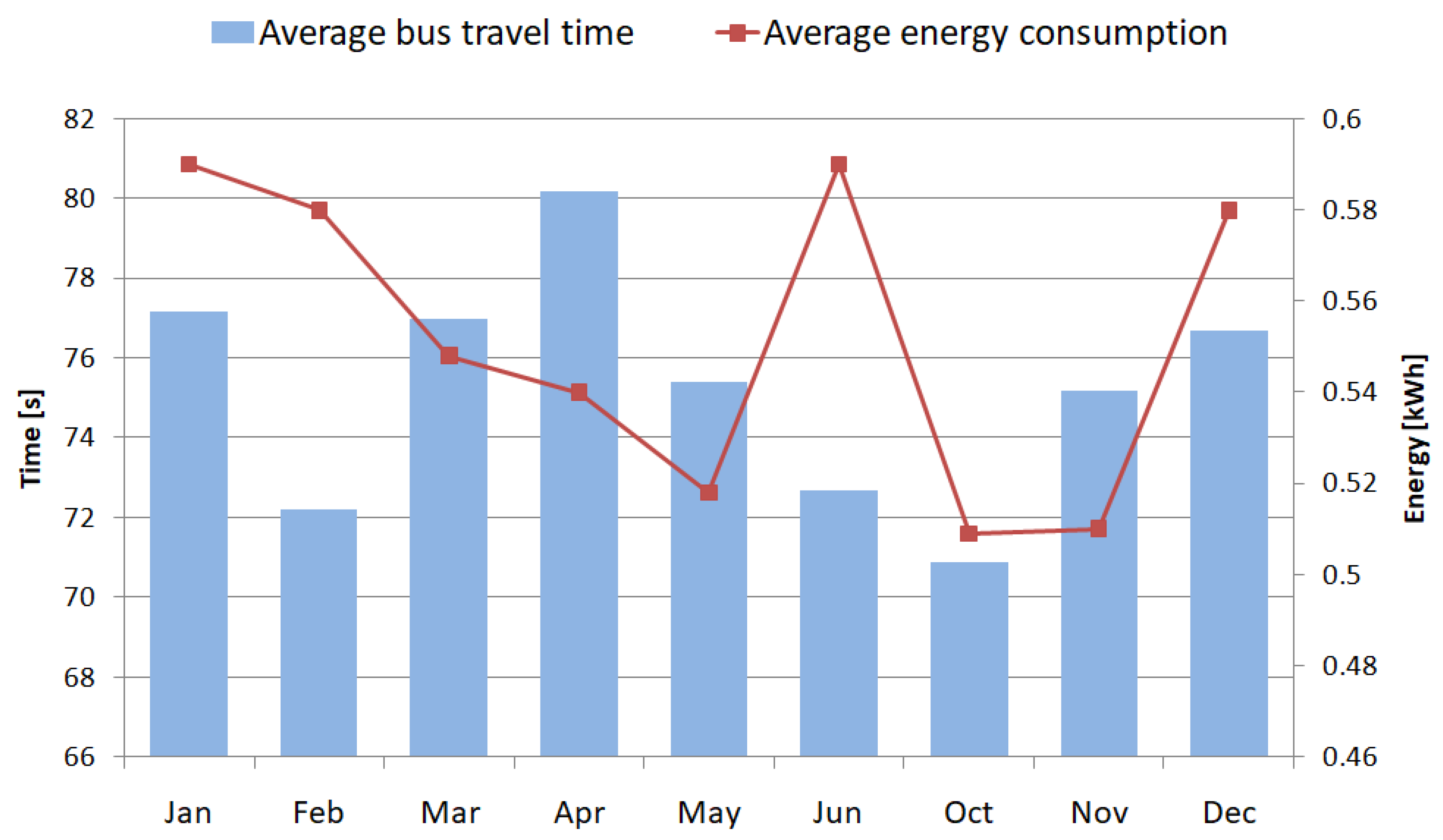
Figure 2 shows the average bus travel time between stops datasets and the average energy consumption datasets between the stops, broken down into individual months in which the data were recorded. It can be seen that energy consumption is not always directly proportional to the time the buses travel between stops and the time they spend at the stops. The weather conditions and the direction of travel (route elevation, up and down) also affect energy consumption. The average values of energy consumption in January and June are very high, mainly due to high utilization of heating systems in winter and air conditioning system in summer. Both systems are very energy-demanding.

The graphs in Figure 2 show the average journey durations and energy consumption for a given month and the same distance between stops of 512 m.

3.2.1. Analysis of Weather Conditions

Average energy consumption depends strongly on the weather conditions. On the days when the data were collected, the temperatures ranged from −5 °C in January to 24 °C in June. The chosen days (one per month) displayed average conditions for the season. In Figure 2 it can be seen that the average energy consumption for journeys in January and June is almost equal (heating in January, air-conditioning in June). For February and December, also, the average energy consumption is similar. For the purposes of the neural network, the weather condition parameter w_n was added to the model. The most energy-demanding months due to weather conditions are coded with the greatest value. For the rest, the value decreases with decrease of energy demand.

Table 2. Weather conditions w_n values.

January	February	March	April	May	June	October	November	December
4	3	2	2	1	4	1	1	3

presents the values assigned to weather condition parameter w_n for each month, after datasets analysis.

3.2.2. Altitude Parameter

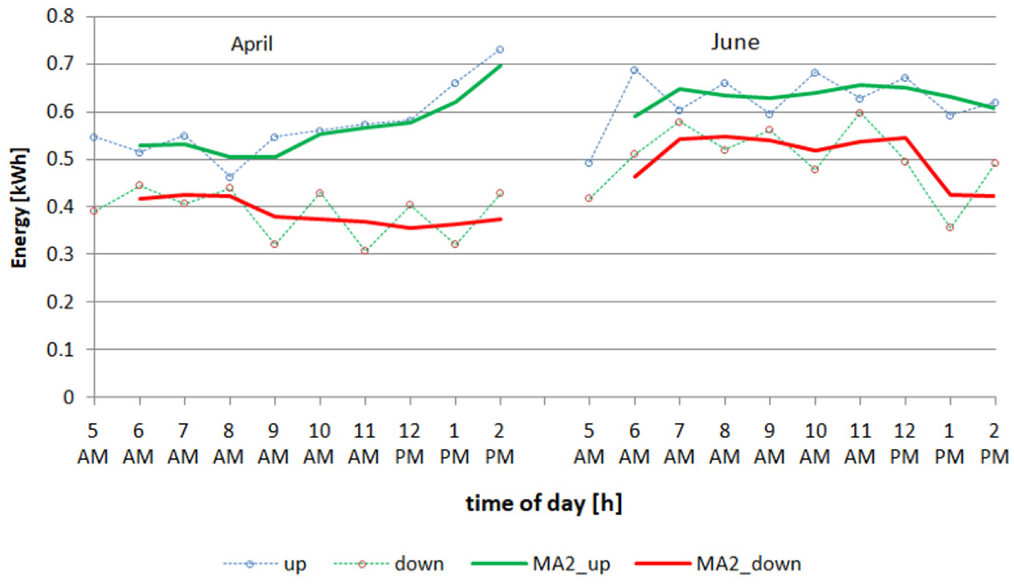
The energy consumption for a bus journey between two stops at a distance of 386 m, for which the elevation difference is 25 m, for two different bus lines was analyzed. The length of the journey in this case is the same in both directions. Figure 3 shows energy consumption under different weather conditions for a direct connection between two stops for round-trip journeys for two days in April and June. In this case, the bus needed about 30% (April) and 20% (June) more energy when going uphill, compared to the energy used when driving downhill. To better show the difference, a moving average has been added in steps of two (MA2—moving average). Up and down lines on the graph represent different bus lines which operate on the same route but in opposite directions.

The graph in Figure 3 also shows that the energy consumption throughout the day (6 a.m.–2 p.m.) differs. The reason may be the uneven road gradient on this section, as well as the greater number of passengers transported at certain times. Number of passengers is reflected by the time the bus spends at the bus stop.

3.2.3. The Peak-Hour Parameter

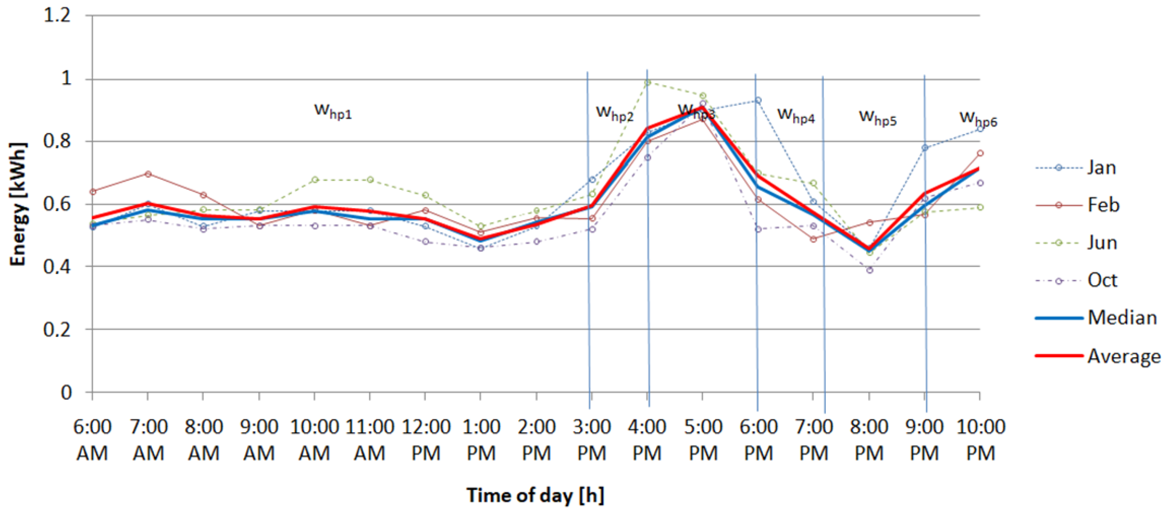
Peak (rush) hours are usually associated with increased energy consumption as the load (number of passengers) on the bus increases. Due to increased number of passengers, not only does load increase, but stops with open doors are also longer, which requires more energy for heating or air-conditioning.

In order to analyze the data in terms of energy consumption during peak hours, the average values and the median of several days of electric bus travels in the summer and winter period were taken into account. Figure 4 shows that the rush hours for analyzed bus lines start at 2.30 p.m. and end around 7.00 p.m. From 9 p.m. onwards, energy consumption starts to increase again.

The entire travel period was divided into six time intervals, and for the purpose of training the neural network, the peak hour parameter thp_n was assigned the values (w_hp1–w_hp2) presented in

Table 3. Peak hours w_hp coding values.

whp1	whp2	whp3	whp4	whp5	whp6
1	2	4	3	1	3

.

The coding values are based on the bus traveling hours and the energy used. The greater the energy value, the greater the coding value determined for a specific time interval.

3.3. Methodology

Based on the analysis of the collected data, the values needed to train and test the neural network for energy consumption estimation were determined. We propose to use five parameters: distance, travel time between consecutive bus stops, road elevation, weather conditions, and peak hours (hour of bus travel).

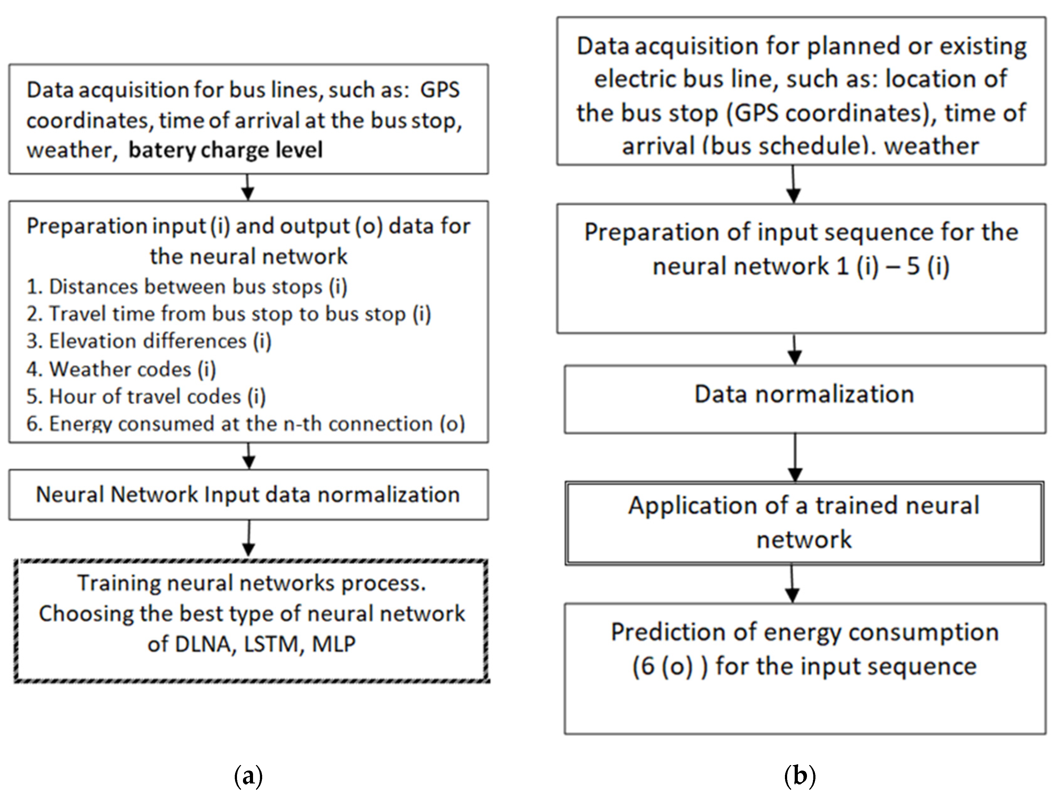
Figure 5a shows the methodology of neural network preparation for the proposed neural energy consumption prediction model. First, GPS coordinates, battery charge levels, and arrival times at bus stops are recorded for a specific bus line. Then, the inputs to our network models need to be normalized and prepared. Finally, one needs to choose the appropriate machine learning method to process the prepared inputs.

Figure 5b shows the method of using a trained neural network to predict energy consumption of an electric bus. In our case, 4600 data samples were collected during travels between stops, 4000 of which were used to train and validate neural networks, and 600 to verify model accuracy.

4. Evaluation of EB Energy Consumption Models Using Various Neural Network Types and Configurations

Thorough analysis of bus travel parameters and their impacts on bus energy consumption yielded the model expressed using the following function:

$$E_n=f\left(d_n,\mathsf{\Delta }{t}_n,\mathsf{\Delta }{h}_n,w_n,tp{h}_n\right),$$

(1)

where

d_n—distances between bus stops;

Δt_n—travel times: time taken to travel between consecutive bus stops;

Δh_n—elevation differences;

w_n—weather conditions;

tph_n—hour of travel codes;

n—the number of the bus trip of a bus line.

The relationships between five variables in Function (1) are nonlinear [28]; thus, the best methods to evaluate it are the deep learning neural network methods. Figure 6 shows a general diagram of the proposed energy consumption model for electric buses.

Different types of networks and their different configurations provide different accuracy of the result. In order to find the best neural network to evaluate the model, a thorough analysis was performed and three types of networks were chosen for comparison: two deep learning networks (DLNA and LSTM) and one multilayer perceptron (MLP) network.

Diagrams of selected networks are presented in Figure 7, Figure 8 and Figure 9, respectively, and their configurations are described below. Research was carried out for all the neural networks mentioned. The input parameters for all the networks are as follows:

• p_n(1)—time Δt_n;
• p_n(2)—distance d_n;
• p_n(3)—elevation differences Δh_n;
• p_n(4)—weather condition w_n;
• p_n(5)—peak hours tph_n,

where n is the n-th bus route section between two stops. The analyzed bus lines are presented in Figure 1. The output of the model is the predicted energy value E_n.

4.1. Deep Learning Networks with Autoencoders (DLNA) Model

The first network studied is a deep learning network with autoencoders. Figure 7 shows a schematic diagram of such a neural network.

The proposed deep learning network consists of a set of stacked autoencoders whose output is passed to a fully connection layer with a backpropagation learning (BP) algorithm from which outputs are passed to the output layer.

The layers are first trained separately; the so-called pretraining is performed, and then, after the initial setting of the weights, combined into one network. Such a network is retrained in order to best match the output value to the input sequence.

Configurations with one or two layers of autoencoders with the number of neurons from 10–50 were tested. In the hidden BP layer, the number of neurons was between 5 and 20. As a result of training and validation, the best configuration, 5-30a-5-1, was selected (5 inputs, 30 neurons in the autoencoder layer, 5 neurons in the BP hidden layer, and one neuron in the output layer).

4.2. Deep Learning LSTM Model

The LSTM network is a special type of recursive network (RNN). The LSTM network is good at mapping correlations between data sequences, especially those representing time series. The LSTM network consists of memory units (memory cells), the structure and operation of which are described in the literature [29].

The LSTM network was used in this study because of its properties. Compared to conventional neural networks, the LSTM network is able to capture the characteristics of the sequence or time series over a longer period of time. Therefore, the prediction evaluation can yield better results when using LSTM networks. Figure 8 shows a diagram of this neural network.

We tested a network consisting of one and two layers of LSTM units containing from 100 to 200 units, and for the fully connection layer (FC) from 10 to 50 neurons. For typical regression tasks, the regression layer should follow the last fully connected layer.

4.3. Multilayer Perceptron Model (MLP)

The MLP type network is a classic neural network that is often used to map linear and nonlinear functional relationships. In this study, it was mainly used for comparison with deep learning networks. It is a one-way network that consists of a series of layers. In the MLP type network, each subsequent layer is connected from the previous layer. The first layer has a connection from the network input. The last layer consists of one neuron; that output is the network’s output—Figure 9.

The backpropagation learning method with the Levenberg–Marquardt fast weight modification algorithm was used for the network. A sigmoid transition function was used in the hidden layers for each neuron. The network with 5-8-8-1 configuration turned out to be the best.

The y_j outputs of the hidden layer neurons are defined as

$$y_j=\frac{1}{1+\exp \left(-s_j\right)},$$

(2)

where s_j is the weighted sum of the network inputs, i.e., p_n(1), p_n(2),…, p_n(k):

$$s_j={\displaystyle \sum }_{i=1}^k\left(w_{ij}{p}_n\left(i\right)+b_j\right)$$

(3)

At the output of the network, the predicted energy value E_n is the sum of the weighted values of the outputs of the neurons of the hidden layer:

$$E_n={\displaystyle \sum }_{j=0}^{M-1}(w_j{y}_j+b),$$

(4)

where M is the number of neurons in the hidden layer.

During learning, the weights of the network inputs and the weights of the neuron outputs of the hidden layer are determined. The operating error (B) of the neural network (objective function) is minimized:

$$B=\frac{1}{n}{\displaystyle \sum }_{i=1}^n{\left(E_{ex}-E_i\right)}^2,$$

(5)

where n—number of training sequence data, E_ex—expected value from the training string for the given input sequence p_n(1), p_n(2), …, p_n(k), E_i—consecutive calculated energy values, i = 1, …, n for the current neuron weights.

The network was trained until the training error 0.001, or to 200 epochs. The learning sequence consisted of 4000 input vectors of five elements and the corresponding output value—energies (E_n), which is output of the neural network, and the learning rate λ = 0.01, momentum α = 0.7.

4.4. Multiple Linear Regression Function (MLR)

A multiple regression function was added to compare the results with neural networks. The coefficients of the MLR were calculated and the values of the regression function were compared with the results of the neural networks. Regression function coefficients were calculated for the same training data that was used to train the neural networks.

Research has shown that the multiple linear regression function can meet the requirements of energy consumption estimation but gives values 1 percentage point (MAPE) worse than the best neural model. In this case, the estimated energy consumption E_n is calculated as follows:

$$E_n=m_1\mathsf{\Delta }{t}_n+m_2{d}_n+m_3\mathsf{\Delta }{h}_n+m_4{w}_n+m_{5}tp{h}_n+b$$

(6)

The results prove that the proposed model may be suitable for estimating energy consumption. The values of the m₁–m₅ coefficients calculated for the set of 4000 data are {3.1265, 0.09206, 0.01622, −0.11534, −0.01336, b = 0.09596}, respectively, which shows that all variables are necessary to calculate the estimates.

5. Results and Discussion

As a result of the verification with the use of non-learning test data, we tested three types of neural networks:

-

Deep learning network with autoencoders (DLNA).

-

Long short-term memory network (LSTM).

-

Classic three-layer feedforward network (MLP).

The network that showed the smallest MAPE and RMSE errors was selected as best for the implementation of the presented energy consumption model. The first neural network configuration used to evaluate the deep learning energy consumption model was one autoencoder, with the number of neurons varying from 10 to 50, and a backpropagation layer, with the number of neurons in the hidden layer ranging from 5 to 10. The training dataset consisted of 4000 sequences of recorded bus travel parameters and the test dataset of 600 sequences. In total, 4600 data samples collected during bus travels between stops were included in the study. Prediction accuracy is evaluated using two errors: root mean square error (RMSE) and mean absolute percentage error (MAPE):

$$RMSE=\sqrt{\frac{1}{n}{\displaystyle \sum }_{i=1}^n{\left(E{r}_i-E_i\right)}^2} MAPE=\frac{1}{n}{\displaystyle \sum }_{i=1}^n\left|\frac{E{r}_i-E_i}{E{r}_i}\right|\ast 100\%$$

(7)

where E_i, Er_i—respectively, predicted and real energy consumption for journey i, n = 600.

RMSE is the square root of the mean of the squares of the differences. It shows how close the observed data values are to the predicted values of the model. Mean absolute percentage error (MAPE) informs about the average magnitude of forecast errors for the test period, expressed as a percentage.

The model evaluation was conducted with the use of the MATLAB 2020a environment (academic license), and computer with Intel(R) Core(TM) i5 2.40 GHz processor, 8 GB of RAM, and with a graphics card NVIDIA GeForce MX330.

Figure 10, Figure 11, Figure 12 and Figure 13 show test results for 100 samples of data from a test dataset of 600 sequences, for sequences 501 to 600. These sequences are selected as representative because they show the greatest number of differences between test results obtained for different network models. The total RMSE and MAPE error values test dataset of 600 sequences are shown in

Table 4. MAPE and RMSE errors for all tested prediction models.

	DLNA	MLP	MLR	LSTM
RMSE (kWh)	0.052	0.056	0.055	0.057
MAPE (%)	6.2	6.7	7.2	7.2
R2	0.973	0.968	0.967	0.966

. The histograms show the distribution of the difference between the actual and predicted values. The RMSE error is the square root of the mean of these differences for the 100 test links.

Figure 10 shows the DLNA test results for the 5-30a-5-1 configuration. Figure 10a compares the values obtained from the network with the actual values. Figure 10b shows a histogram of the difference between the actual and predicted values corresponding to the left-hand graph. It can be seen that many of the predicted values underestimated the actual energy consumption values. Underestimated values (the difference between the actual and predicted value is greater than zero) in this case constitute 65% of all tested data. These dependencies can also be observed in Figure 10a. The red line shows the data predicted by the DLNA network. The RMSE error for this 100-element test set is 0.038 kWh.

Next, the LSTM network was analyzed. Figure 11 shows the results of the LSTM network test for the 5-200u-1 configuration (five inputs, 200 LSTM units and 1 neuron) in the FC layer.

In the case of this network, the number of cases for which the difference between the actual and predicted values is greater than zero is similar to the opposite cases and amounts to 51%. The RMSE error for this 100-element test set is 0.054 kWh.

Finally, MLP network results were analyzed. Figure 12 shows the results of the MLP network test for the 5-8-8-1 configuration (five input values, eight neurons in the first hidden layer, eight neurons in the second hidden layer, and one neuron in the output layer).

This network, similar to the DLNA network, predicts a lower energy value than the real one in 61% of 100 test data. The RMSE error for this 100-element test set is 0.045 kWh.

Additionally, MLR function results were compared to the ones obtained from neural networks. Figure 13 shows the test results for the multiple linear regression function (MLR). The histogram shows that the most data from the test set was estimated with an error of −0.05 kWh, i.e., the values were higher than the real. However, the average frequency shows that out of 100 connections, 50% of the values were higher and the remainder were lower than the real.

The RMSE error for sequences 501 to 600 is 0.052 kWh.

Total MAPE and RMSE error was calculated for 600 test sequences. The values of MAPE and RMSE errors obtained for all described above networks and functions are presented in Table 4.

RMSE is an absolute measure of fit and R² is a relative measure of fit. For predictive models, RMSE is one of the most important indicators of the quality of fit.

In Table 4, the DLN model has the lowest value of 0.052 kWh, which means the best fit of the model to the data. The best coefficient of determination R² also reached a value of 0.973 for the model with the DLNA network.

The MAPE value allows you to compare the accuracy of the forecasts of different models. In Table 4, the lowest value of the MAPE error equal to 6.2% was also obtained for the DLNA model. In general, it can be said that all models give good accuracy. The values of 6.7% for the MLP model and 7.2% for the LSTM and MLR models are also very good results.

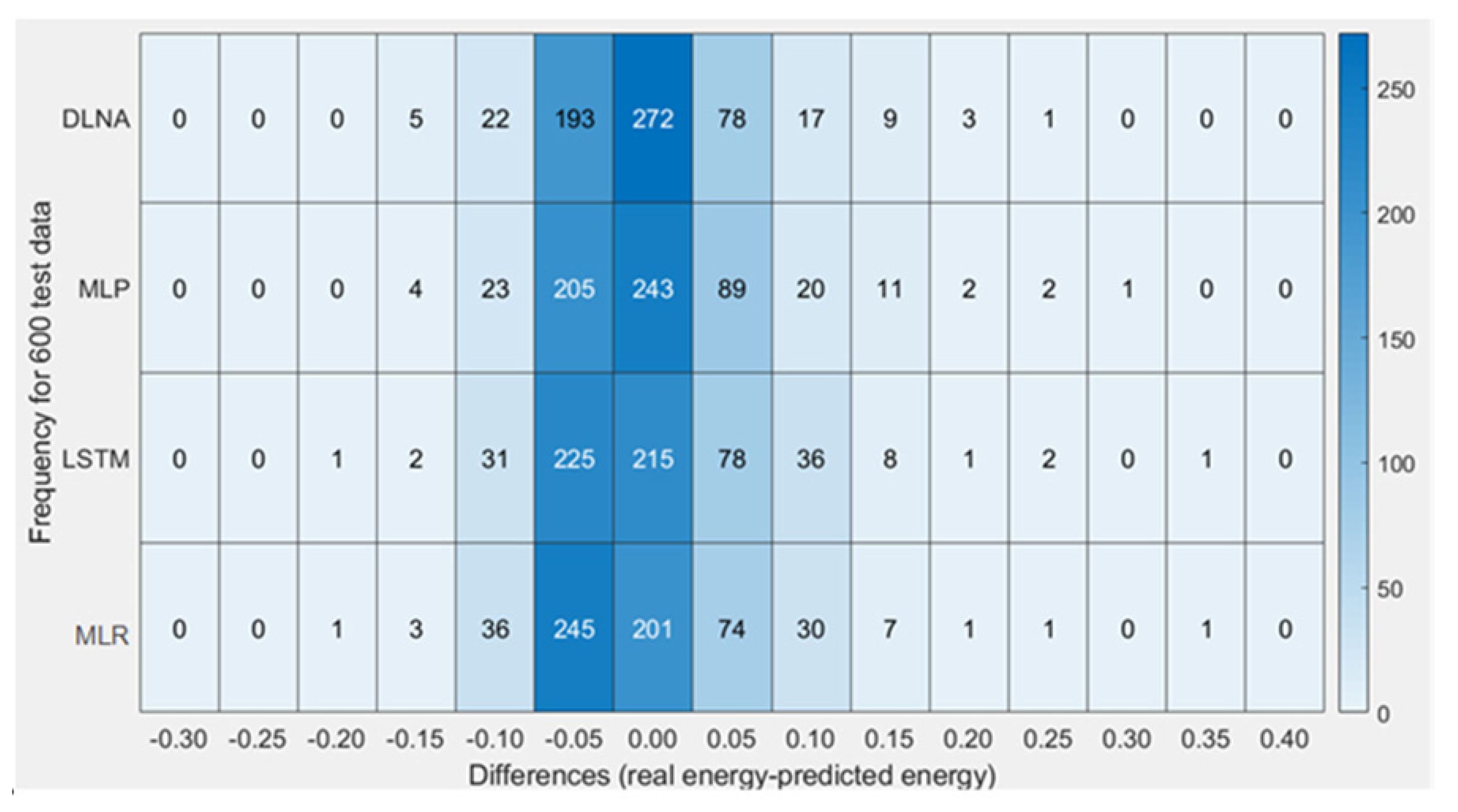
Figure 14 shows the frequency distribution of the relative errors for all tested models. The largest number of predicted energy values for the test data with an error close to zero occurred for the DLNA network. Second in terms of the accuracy of estimating energy consumption models is the MLP; the other models gave very similar results.

Better results could be expected for the recently popular LSTM network. However, the LSTM network gives the best results for the time series. The five parameters used to estimate the amount of energy consumed can be time series; however, they are short sequences for journeys between the same stops or several bus connections. It can be assumed that this type of network would give better results if the obtained data were grouped into time series. However, this is a broad topic for another study.

The accuracy of the model is highly dependent on the test data. To illustrate the obtained results even better, the graph in Figure 15 shows the MAPE error plot for the test set divided into three groups of 200 sequences, from 1–200, 201–400, and 401–600.

For these three groups, the best results were still achieved with the DLNA model. The MAPE error for this model for sequences from 1–200, 201–400, and 401–600 was 5.76%, 6.57%, and 6.41%, respectively (on average 6.2%), and these are the lowest values in relation to other models.

Finally, we have compared new results with the ones obtained for the first version of the model described in [13]. Both results are shown in

Table 5. MAPE and RMSE errors for two models.

	DLNA	MLR	DLNA *	MLR *
RMSE [kWh]	0.052	0.055	0.077	0.085
MAPE [%]	6.2	7.2	7.1	8.2
R2	0.973	0.967	0.944	0.935

* Results for four input parameters [13].

.

It can be seen that MAPE values obtained for the new model are better than the previous ones, and the difference is around 1%. The additional input parameter also improved values of RMSE and R². Overall, the accuracy of the new model is better, and the cost of obtaining the new parameter is negligible as it is also a readily available parameter.

6. Conclusions

The article describes efficient application of the energy prediction of electric buses problem to neural networks which can provide high accuracy of the result. The authors propose a neural network model for estimating energy consumption by an electric bus traveling within the city. The model uses readily available bus travel parameters, thus avoiding additional expenses for bus operators, e.g., for specialized measurement equipment. The model input parameters are data that are normally available to the bus operator. There are no special speed profiles or detailed information about the technical data of the electric bus or installation of specialized, costly measuring equipment. Thus, the model can efficiently serve bus operators when introducing electric buses and planning charging infrastructure.

The suitability of three types of neural networks for the purpose of model validation was tested. The training sequence consisted of 4000 sequences, which represented 4000 bus connections between over 100 stops on two bus lines in the city of Jaworzno in Poland. The test dataset consisted of 600 sequences that were not a subset of the training set.

The best results were achieved for deep learning networks with autoencoders (DLNA). The MAPE error for this network is 6.2%, and the other networks gave the accuracy of 6.7% (MLP) and 7.2% (LSTM). Additionally, the results obtained with the use of neural networks with the linear regression function were compared, and an error of 7.2% was obtained for the same test data. As can be observed, the model is very efficient even with less computationally heavy methods, i.e., MLR. Thus, if smaller accuracy is accepted and very low cost of prediction is required, then the model can be evaluated with MLR, still providing good energy demand estimation.

The experimental results showed that the proposed model is very accurate, and its accuracy exceeds the accuracy of models based on other types of neural network and analytical models that require a lot of additional data.

Although all neural network types are able to map nonlinear dependencies as defined in Function (1), the conducted study yields that the selection of the appropriate type of network impacts the accuracy of estimation of energy consumed by an electric bus.

It was verified that adding additional parameter to the model increases its accuracy by 1% (MAPE).

We are negotiating with other bus companies which operate in bigger cities in order to acquire new datasets for future analysis and research on the matter. We plan to assess the importance of additional parameters on energy prediction.

We plan to analyze the impact of other parameters on the accuracy of the prediction, such as instantaneous speed, auxiliary loads, and technical condition of the vehicle. Furthermore, we would like to analyze the impact of road incidents on reliability of the model.

The obtained model and its validation results can form the basis for further research on charging strategies and requirements related to the charging infrastructure.