Microgrid Operation Optimization Using Hybrid System Modeling and Switched Model Predictive Control

Abstract

Optimization of economic aspects of microgrid operation in both grid-connected and islanded mode leads to contradictive definitions of optimality for both modes. There is no general agreement on how to cope with this duality. To address this issue, as well as modern energy market requirements and a better renewable energy utilization necessity in the case of large facilities, a comprehensive control solution utilizing the appropriate model is needed. In response, the authors propose a hybrid microgrid model covering fundamental features and designed to work in conjunction with two switched receding horizon control laws. A relevant controller is chosen according to the current microgrid operation mode and its cost function tailored to specific demands of the islanded or grid-connected operation. Performed research led to a new switched hybrid model predictive control approach focused on microgrid economic optimization. This approach utilizes an appropriate hybrid microgrid model also contributed by the authors. The introduced solution turned out to be effective in overall energy cost reduction in the case of large commercial facilities, regardless of grid-connection and renewable generation scenarios. Furthermore, it also provides satisfactory renewable energy and storage capabilities utilization in changing grid connection conditions.

1. Introduction

Recent policy for climate and energy leans towards reducing greenhouse gas emissions and reaching energy systems without a significant carbon footprint. Electricity generation and consumption are at the forefront of this change. Therefore, currently used distribution and transmission grids will have to inevitably meet the above-mentioned requirements and a key solution in achieving carbon-neutral smart grids seem to be wide usage of microgrid solutions [1]. To reach that neutrality, a vast amount of renewable energy sources is vital and transition to such means of energy production is already taking place. Unfortunately, as pinpointed in [2], the adoption of renewable energy sources pose various challenges arising from user demands and fluctuate profiles of renewable energy generation far different from traditional means of energy generation. The structural solution to those new challenges is splitting the electrical network into smaller units based on distributed resources. Every smaller segment, the so-called microgrid, manages the local loads, generation and is equipped with storage capabilities. Moreover, it possesses means of connecting to and disconnecting from other segments, as well as can exchange energy with them. This approach significantly improves possibilities of remedying the instability of renewable sources and allows for fuller utilization of available renewable energy. In addition, small independent networks capable of island-mode operation tend to be incomparably more reliable in terms of continuity of supply and, with appropriate control strategies, offer economical benefits not only in remote regions.

According to [3], when considering complex microgrid control solutions, hierarchical control is mainly selected. Such systems consist of three distinguishable levels. Primary control stabilizes system frequency and voltage in response to rapid load changes, thus operating on the smallest timescale. Secondary control focuses on nullifying grid parameters deviations in steady-state and synchronizing with the public grid after the transition to grid-connected operation. Lastly, tertiary control is responsible for power flow control between microgrid elements or between microgrid clusters and upstream, public grid. Additionally, it introduces further functionalities in form of large-scale planning or economic optimization. As reported in [4], microgrid management is often associated with optimal control or optimization. Such optimization may concern economic, environmental, or technical objectives and optimal operation can be achieved using various techniques. Frequently used approaches include meta-heuristic or heuristic methods, stochastic and robust methods, Model Predictive Control in various forms, linear, dynamic, and nonlinear programming, as well as artificial intelligence.

Single and multi-objective optimization methods based on heuristic algorithms such as particle swarm or firefly optimization are a widespread choice. Some of the usage cases include cost and sizing optimization with fossil fuel share reduction in energy generation [5], microgrid load dispatch optimization [6] and for optimization of energy production cost in a microgrid [7]. Meta-heuristics are also used in combination with other techniques such as mixed-integer linear programming [8] or artificial neural networks [9]. On the other hand, artificial neural networks can adapt to uncertainties and are applicable when the exact model of a system is not available [10]. Exemplary applications include optimal energy scheduling [11] and storage system management [12]. It is worth noting that, according to [10], artificial neural networks are more commonly used in primary and secondary control than on the tertiary level. An exemplary solution utilizing a fuzzy-logic decision system in a multi-objective optimization problem can be found in [13]. Due to uncertainties, such as energy demand and generation, robust and stochastic optimization and control algorithms are also applicable in microgrid management cases. Robust optimization focused on both economy and robustness is presented in [14]. An exemplary optimal stochastic energy management system can be found in [15] and a robust economic energy and reserve management system is derived in [16]. Lastly, different mathematical programming methods are widely used, including dynamic, mixed-integer, and nonlinear programming. Some of the usage cases include energy generation cost optimization [17] and demand-generation mismatch optimization [18]. Importantly, the latter two are often equated with hybrid and nonlinear Model Predictive Control. Given the focus of this paper, usage of Model Predictive Control and mixed-integer linear programming, especially in hybrid form, will be discussed in detail below.

The applicability of Model Predictive Control (MPC in short) on all microgrid control levels is one of its most significant advantages. As reported in [19,20], the popularity of MPC stems from the fact that the resulting control strategy, due to the direct use of the process model, respects all system interactions and constraints which are not that easy to capture using other control methods. Moreover, it provides constraints satisfaction, stability guarantee and is adequate in application to multi-variable processes. Going back to the microgrid world, it is clear that any microgrid consists of a substantial amount of interacting elements, sometimes in an unintuitive manner, and controllers must operate in a significantly constrained environment. Interestingly, various phenomenons occurring in microgrid exhibit hybrid behavior, therefore building microgrid hybrid models is not overly complicated, especially in the economical scope. Additionally, receding horizon control is highly compatible with hybrid systems and such a combination is widely used. In [21], a hybrid model is used for economical optimization to include as much detail as possible and conventional MPC is used in form of a single mixed-integer linear programming (MILP) problem among other methods. The scope of research is focused on grid-connected mode and islanded operation is not considered. A Single Hybrid MPC (HMPC) solution using Mixed Logical Dynamical (MLD in short) framework in conjunction with a highly efficient MILP solver is presented in [22]. The scope of modeling focuses on economic and dynamic modeling of microgrid components including varying energy costs taken into account during optimization but no demand-side management. The exact solution is dedicated to the Brazilian energy market. In turn, the authors of [23] aim to design a management system dedicated to smart house systems. A hybrid model of its electrical and thermal system is derived, HMPC for on-grid operation proposed and solved using MILP solver. Importantly, a time-varying energy price is also introduced and no demand-side management is considered. As can be seen, the usage of mixed-integer linear programming is very wide, mainly because of highly accessible and efficient solvers, as well as simulation environments equipped with toolboxes connecting solvers and hybrid modeling tools. The synergy between microgrid modeled using discrete hybrid automata described in HYSDEL language and resulting MILP solved using CPLEX solver is precisely described in [24] where authors propose a hybrid optimization model for management of microgrid featuring automatic grid connection. A similar approach is presented in [25]. The study presents a hybrid model predictive control solution to optimal economic energy management of microgrid with hydrogen-based storage. Applied control scheme employs single Lyapunov-based HMPC using microgrid model in discrete hybrid automata form converted to MLD representation. Demand-side management is not considered and emphasis is put on grid-connected operation. The solution includes optimal dispatch and load sharing controllers. Naturally, there are other usable optimization approaches, without the introduction of receding control strategies in form of MPC. The authors of [26] use particle swarm optimization with the aim of minimizing the operation cost of a microgrid and improving photoelectric consumption by means of energy demand management. The algorithm is also solving a single MILP problem. Varying energy price is used but the microgrid remains connected to the public grid.

Considering the wide range of MILP applications and available tools authors of this paper choose to develop a novel HMPC-based control solution covering separate optimization of both on-grid and off-grid operation. To clarify, when dealing with microgrid switching between on-grid and off-grid operation mode, the control system must achieve an optimal solution regardless of the current mode. However, optimal control for each of those modes should be reached using different criteria resulting in slightly different optimization problems but still using the same microgrid model. That said, derivation of compatible microgrid hybrid model was also needed. Moreover, such a model should also cover demand-side management and the presence of energy-tariff with changing energy price.

A novel control concept utilizing switched hybrid MPC applied to economically optimize microgrid operation is the main contribution of this paper. Additionally, a compatible hybrid microgrid model in MLD form featuring demand-side management, varying energy price, and operation in both grid-connected and islanded mode is also contributed.

2. Economically Oriented Microgrid Hybrid Model

To date, various methods have been applied to model different aspects of microgrid operation. The general use of hybrid modeling is a well-established approach to capturing phenomenons occurring in a microgrid, understood as a dynamical system. Those phenomenons tend to be nonlinear or highly complicated and, what follows, problematic to directly model. This also entails high computational cost which is vital for model predictive control-oriented applications. Segmenting complex relationships into relatively simple pieces and switching them depending on certain conditions proves very useful, especially in the case of microgrids. Multiple distinguishable microgrid components are naturally operating in a hybrid manner, for example, energy storage is either discharged or charged, depending on energy demand and supply balance. The authors decided on employing a hybrid microgrid model in the mixed logical dynamical form given reduced computational burden and high compatibility with phenomenons occurring in a microgrid, as well as with model predictive control. This section introduces a hybrid model built to work in conjunction with the proposed switched MPC control approach.

2.1. Energy Storage Description

The derived energy storage model is based on the simple principle of energy balance sourced from [21] and expanded. Variable $E_{st}(k+1)$ represents energy aggregated in energy storage at time $k+1$, which depends on current storage level $E_{st}\left(k\right)$, constant self-discharge $E_{sd}$, energy discharged from storage $\frac{1}{{\eta }_d}{E}_{-}$ and amount of energy charging the storage ${\eta }_c{E}_{+}$. Charging and discharging efficiency is taken into account and labelled as ${\eta }_c$ and ${\eta }_d$, respectively. Equation (1) describes the aforementioned relationship:

$$E_{st}(k+1)=E_{st}\left(k\right)+{\eta }_c{E}_{+}\left(k\right)-\frac{1}{{\eta }_d}{E}_{-}\left(k\right)-E_{sd}$$

(1)

Energy charging the storage unit is described as previous energy balance in microgrid $E_b(k-1)$ multiplied by boolean ${\delta }_b$ which indicates positive or negative $E_b(k-1)$ as follows:

$$E_{+}\left(k\right)=\left\{\begin{array}{c}{E}_b(k-1)\mathrm{for}{\delta }_b\left(k\right)\left(z_{\mathit{ex}}\left(k\right)\right)\hfill \\ 0\mathrm{otherwise}\hfill \end{array}\right.$$

(2)

where $z_{ex}\left(k\right)$ denotes auxiliary variable defined as a product of the real variable $E_b(k-1)$ and the logical condition ${\delta }_b$. It is equivalent to the expression $z_{ex}\left(k\right)={\delta }_b\left(k\right)E_b(k-1)$. A similar notation will be used throughout the whole model description. Charging delay is added to take into account that storage charging or discharging is not instant. Furthermore, energy discharged is expressed as previous energy balance $E_b(k-1)$ minus already explained $E_{+}\left(k\right)$:

$$E_{-}\left(k\right)=E_b(k-1)-E_{+}\left(k\right)$$

(3)

Substitution of $E_{+}\left(k\right)$ and $E_{-}\left(k\right)$ to Equation (1) reveals that ${\delta }_b$ is used to nullify or include certain expressions depending on energy balance. This means that, given negative $E_b\left(k\right)$, auxiliary binary variable ${\delta }_b\left(k\right)$ becomes zero and storage is discharged with efficiency ${\eta }_d$. On the other hand, in the case of non-negative energy balance, hence ${\delta }_b\left(k\right)$ equal one, storage is charged with the efficiency ${\eta }_c$. Finally, self-discharge constant $E_{sd}$ consists of energy spent to cool storage units labeled as $E_{ac}$ and energy lost due to natural self-discharge $E_{nd}$:

$$E_{sd}=E_{ac}+E_{nd}$$

(4)

Appropriate $E_{ac}$ and $E_{nd}$ values are adopted based on informations from [27].

2.2. Transactions with a Public Energy Network

Other essential components of a microgrid model are energy transactions with a public energy network. Considering an economically oriented approach, those can be understood as costs and gains associated with buying and selling energy, respectively. At this point, it should be emphasized that authors assume energy purchase prices change over time according to the energy tariff given in [28], which is currently available in Poland. Figure 1 shows the resulting energy price chart.

As can be seen from Figure 1, three pricing periods can be distinguished: standard price $f_{flat}$, morning peak price $f_{mp}$ and evening peak price $f_{ep}$. Introduction of a simple timer $t_{tim}$ is necessary for the model to correctly switch between aforementioned prices. Time aggregated in $t_{tim}$ is increased at every time step k by sampling time $T_s$ and reset, by subtracting 24, if boolean ${\delta }_{tim}\left(k\right)$ indicates that $t_{tim}\left(k\right)$ is equal or greater than 24. This relationship is specified by:

$$\begin{array}{c}\hfill t_{tim}(k+1)=t_{tim}\left(k\right)+T_s-z_{tim}\left(k\right)\end{array}$$

(5)

$$\begin{array}{c}\hfill t_{tim}\left(k\right)\ge 24⟺{\delta }_{tim}\left(k\right)=1\end{array}$$

(6)

$$\begin{array}{c}\hfill z_{tim}\left(k\right)=24{\delta }_{tim}\left(k\right)\end{array}$$

(7)

That simple timer made switching between energy prices according to the current time possible. However, actual energy price switching is based on inequalities and binary auxiliary variables ${\delta }_{t1}\left(k\right)$, ${\delta }_{t2}\left(k\right)$, ${\delta }_{t3}\left(k\right)$ and ${\delta }_{t4}\left(k\right)$ becoming true when certain time has been exceeded. Variables $t_{mps}$ and $t_{mpe}$ indicate starting and ending time of morning peak, respectively. Similarly, $t_{eps}$ and $t_{epe}$ correspond with the evening peak as follows:

$$\begin{array}{cc}\hfill t_{tim}\left(k\right)\ge t_{mps}& ⟺{\delta }_{t1}\left(k\right)=1\hfill \end{array}$$

(8)

$$\begin{array}{cc}\hfill t_{tim}\left(k\right)\le t_{epe}& ⟺{\delta }_{t2}\left(k\right)=1\hfill \end{array}$$

(9)

$$\begin{array}{cc}\hfill t_{tim}\left(k\right)\ge t_{eps}& ⟺{\delta }_{t3}\left(k\right)=1\hfill \end{array}$$

(10)

$$\begin{array}{cc}\hfill t_{tim}\left(k\right)\le t_{mpe}& ⟺{\delta }_{t4}\left(k\right)=1\hfill \end{array}$$

(11)

In addition, the amount of energy exchanged with the public grid is denoted by $E_{ex}$ and related auxiliary variable ${\delta }_{ex}$, describing its sign, defined in the following way:

$$E_{ex}\left(k\right)\ge 0⟺{\delta }_{ex}\left(k\right)=1$$

(12)

Then, using timing taken from Equation (9) through Equation (11) and pricing according to Figure 1, variability of base energy cost $c_c\left(k\right)$ can be expressed as:

$$c_c\left(k\right)=\left\{\begin{array}{cc}{E}_{ex}\left(k\right)f_{mp}\mathrm{for}{\delta }_{t1}\left(k\right)\wedge {\delta }_{t4}\left(k\right)\wedge {\delta }_{\mathit{ex}}\left(k\right)\wedge {\delta }_{\mathit{cp}}\hfill & \left(z_{\mathit{mp}}\left(k\right)\right)\hfill \\ E_{ex}\left(k\right)f_{ep}\mathrm{for}{\delta }_{t2}\left(k\right)\wedge {\delta }_{t3}\left(k\right)\wedge {\delta }_{\mathit{ex}}\left(k\right)\wedge {\delta }_{\mathit{cp}}\hfill & \left(z_{\mathit{ep}}\left(k\right)\right)\hfill \\ E_{ex}\left(k\right)f_{flat}\mathrm{for}\sim ({\delta }_{t1}\left(k\right)\wedge {\delta }_{t4}\left(k\right))\wedge \sim ({\delta }_{t2}\left(k\right)\wedge {\delta }_{t3}\left(k\right))\wedge {\delta }_{\mathit{ex}}\left(k\right)\wedge {\delta }_{\mathit{cp}}\hfill & \left(z_{\mathit{flat}}\left(k\right)\right)\hfill \\ 0\mathrm{otherwise}\hfill & \end{array}\right.$$

(13)

At last, the total energy purchase cost is defined as an aggregate of various fees, multiplied by the amount of energy exchanged with the public grid $E_{ex}\left(k\right)$. Besides, according to [28], total energy cost $c_b\left(k\right)$ consists of switched base energy cost $c_c\left(k\right)$, co-generation fee $f_{cg}$, renewable energy fee $f_{res}$, quality fee $f_q$ and switched power cost $c_p\left(k\right)$ further associated with the power fee $f_p$, hence:

$$c_b\left(k\right)=E_{ex}\left(k\right)(f_{cg}+f_{res}+f_q)+c_c\left(k\right)+c_p\left(k\right)$$

(14)

with $c_p\left(k\right)$ defined as:

$$c_p\left(k\right)=\left\{\begin{array}{cc}{E}_{ex}\left(k\right)f_p\hfill & \mathrm{for}{\delta }_{t1}\left(k\right)\wedge {\delta }_{t2}\left(k\right)\wedge {\delta }_{\mathit{ex}}\left(k\right)\wedge {\delta }_{\mathit{cp}}\left(z_p\left(k\right)\right)\hfill \\ 0\hfill & \mathrm{otherwise}\hfill \end{array}\right.$$

(15)

Note that binary variable ${\delta }_{cp}$ is associated with the grid connection status. Consequently, when in on-grid mode, ${\delta }_{cp}$ equals one and in off-grid mode, its value changes to zero.

On the contrary, profit from selling excessive energy $c_s\left(k\right)$ is described by significantly simpler Equation (16). Given negative $E_{ex}\left(k\right)$ indicated by ${\delta }_{ex}\left(k\right)$ equal to zero and active connection with public grid due to ${\delta }_{cp}\left(k\right)=1$, energy is sold at price $f_{sell}$. If at least one of those conditions is not met, the microgrid is not connected to public grid or is buying the energy, therefore $c_s\left(k\right)$ is set to zero.

$$c_s\left(k\right)=\left\{\begin{array}{cc}-E_{ex}\left(k\right)f_{sell}\hfill & \mathrm{for}\sim {\delta }_{\mathit{ex}}\left(k\right)\wedge {\delta }_{\mathit{cp}}\left(k\right)\left(z_s\left(k\right)\right)\hfill \\ 0\hfill & \mathrm{otherwise}\hfill \end{array}\right.$$

(16)

As a result, profit $c_s\left(k\right)$ equals the amount of sold energy multiplied by the constant energy selling price. Appropriate energy selling price is taken from [29] and converted to euros.

2.3. Critical and Non-Critical Energy Demand

The aforementioned microgrid energy balance takes into account two main load sources. Both critical $E_c\left(k\right)$ and non-critical $E_n\left(k\right)$ loads are given as sum of various lesser loads:

$$\begin{array}{c}\hfill E_c\left(k\right)=\sum _{i=1}^n{E}_c{}_i\left(k\right)\end{array}$$

(17)

$$\begin{array}{c}\hfill E_n\left(k\right)=\sum _{i=1}^n{E}_n{}_i\left(k\right)\end{array}$$

(18)

Due to the fact that non-critical loads are also controllable, it is necessary to introduce a demand reduction coefficient $\beta \left(k\right)$. This also poses a problem because $\beta \left(k\right)$ is considered as an input and disturbance $E_n\left(k\right)$ is treated as a state variable. By definition, every equation forming part of a mixed logical dynamical model must be affine and hence multiplication and division of inputs, outputs, and state variables are not permitted. In other words, it has become necessary to approximate the product of controllable loads summary demand $E_n\left(k\right)$ and demand reduction coefficient $\beta \left(k\right)$. The main idea is to restrict the range of values of $\beta \left(k\right)$ to predefined, fixed values of ${\beta }_{apx}$ by checking in what range $\beta$ lies at time k, store the results of performed checks in binary variables ${\delta }_{b1}\left(k\right)\dots {\delta }_{b6}\left(k\right)$ defined as follows:

$$\begin{array}{c}\beta \left(k\right)\ge {\beta }_{apx1}⟺{\delta }_{b1}\left(k\right)=1\hfill \end{array}$$

(19)

$$\begin{array}{c}\beta \left(k\right)\ge {\beta }_{apx2}⟺{\delta }_{b2}\left(k\right)=1\hfill \end{array}$$

(20)

$$\begin{array}{c}\beta \left(k\right)\ge {\beta }_{apx3}⟺{\delta }_{b3}\left(k\right)=1\hfill \end{array}$$

(21)

$$\begin{array}{c}\beta \left(k\right)\ge {\beta }_{apx4}⟺{\delta }_{b4}\left(k\right)=1\hfill \end{array}$$

(22)

$$\begin{array}{c}\beta \left(k\right)\ge {\beta }_{apx5}⟺{\delta }_{b5}\left(k\right)=1\hfill \end{array}$$

(23)

$$\begin{array}{c}\beta \left(k\right)\ge {\beta }_{apx6}⟺{\delta }_{b6}\left(k\right)=1\hfill \end{array}$$

(24)

and round original $\beta \left(k\right)$ down to predefined values of ${\beta }_{apx1}\dots {\beta }_{apx6}$ in accordance with the following rules:

$$E_{napx}\left(k\right)=\left\{\begin{array}{cccc}{E}_n\left(k\right){\beta }_{apx1}\hfill & \mathrm{for}\hfill & {\delta }_{b1}\left(k\right)\wedge \sim {\delta }_{b2}\left(k\right)\hfill & \left(z_{\mathrm{apx}1}\left(k\right)\right)\hfill \\ E_n\left(k\right){\beta }_{apx2}\hfill & \mathrm{for}\hfill & {\delta }_{b2}\left(k\right)\wedge \sim {\delta }_{b3}\left(k\right)\hfill & \left(z_{\mathrm{apx}2}\left(k\right)\right)\hfill \\ E_n\left(k\right){\beta }_{apx3}\hfill & \mathrm{for}\hfill & {\delta }_{b3}\left(k\right)\wedge \sim {\delta }_{b4}\left(k\right)\hfill & \left(z_{\mathrm{apx}3}\left(k\right)\right)\hfill \\ E_n\left(k\right){\beta }_{apx4}\hfill & \mathrm{for}\hfill & {\delta }_{b4}\left(k\right)\wedge \sim {\delta }_{b5}\left(k\right)\hfill & \left(z_{\mathrm{apx}4}\left(k\right)\right)\hfill \\ E_n\left(k\right){\beta }_{apx5}\hfill & \mathrm{for}\hfill & {\delta }_{b5}\left(k\right)\wedge \sim {\delta }_{b6}\left(k\right)\hfill & \left(z_{\mathrm{apx}5}\left(k\right)\right)\hfill \\ E_n\left(k\right){\beta }_{apx6}\hfill & \mathrm{for}\hfill & {\delta }_{b6}\left(k\right)\hfill & \left(z_{\mathrm{apx}6}\left(k\right)\right)\hfill \end{array}\right.$$

(25)

The resulting expressions are affine and further applicable to the energy balance equation. Figure 2 illustrates the methodology set out above through a simple example.

2.4. Power Generator and Energy Balance in Microgrid

It was decided that there would be a deadband on power generator power to mitigate inconsiderable power values resulting in unnecessary generator activation. Therefore, generator power $P_g\left(k\right)$ is checked if lower than the deadband $P_{db}$ and the result is stored in ${\delta }_{db}\left(k\right)$. In case of the power demanded from the generator at time k being less than or equal to $P_{db}$, boolean ${\delta }_{db}\left(k\right)$ is set to zero as set out below:

$$P_g\left(k\right)\le P_{db}⟺{\delta }_{db}\left(k\right)=1$$

(26)

Moreover, the usage of a power generator bears some costs which cannot be omitted. Overall generator operation cost $c_{mg}$ is composed of fuel cost approximated by means of expression $z_{fa1}\left(k\right)-z_{fa2}\left(k\right)$ and constant maintenance cost $c_{mnt}$. The generator state is described using boolean ${\delta }_g\left(k\right)$, with zero indicating that it is not providing any power. As a result, $c_{mg}\left(k\right)$ is described as:

$$c_{mg}\left(k\right)=z_{fa1}\left(k\right)-z_{fa2}\left(k\right)+z_{mnt}\left(k\right)z_{mnt}\left(k\right)=c_{mnt}{\delta }_g\left(k\right)$$

(27)

It is worth noting that when generator power output lies under specified threshold $P_{tr}$, checked through the following inequality:

$$\begin{array}{c}\hfill P_g\left(k\right)\le P_{tr}⟺{\delta }_{tr}\left(k\right)=1\end{array}$$

(28)

fuel cost is independent to $P_g$ and set using $f_{const}$. Otherwise, linear approximation using coefficients $f_a$, $f_b$ and fuel price $f_{fd}$ gets chosen. However, the partial fuel cost $z_{fa2}\left(k\right)$ is solely used to nullify the influence of $f_{const}$ on the fuel cost when above the threshold value. The aforementioned functionality is introduced using Equations (29) and (30).

$$\begin{array}{c}\hfill z_{fa1}\left(k\right)=\left\{\begin{array}{cc}{f}_{const}{f}_{fd}{T}_s\hfill & \mathrm{for}{\delta }_{\mathrm{tr}}\left(k\right)\hfill \\ (f_a{P}_g\left(k\right)+f_b)f_{fd}{T}_s\hfill & \mathrm{otherwise}\hfill \end{array}\right.\end{array}$$

(29)

$$\begin{array}{c}\hfill z_{fa2}\left(k\right)=\left\{\begin{array}{cc}{f}_{const}{f}_{fd}{T}_s\hfill & \mathrm{for}{\delta }_{\mathrm{tr}}\left(k\right)\wedge \sim {\delta }_g\left(k\right)\hfill \\ 0\hfill & \mathrm{otherwise}\hfill \end{array}\right.\end{array}$$

(30)

Generator startup and shutdown is also to be penalized using already mentioned boolean generator status ${\delta }_g\left(k\right)$, with $c{s}_{SD}$ and $c{s}_{SU}$ being two cost coefficients, respectively, for shutdown and startup. Therefore, the resulting cost $c_{st}\left(k\right)$ is defined as:

$$c_{st}\left(k\right)=c{s}_{SD}(\sim {\delta }_g\left(k\right)\wedge {\delta }_g(k-1))+c{s}_{SU}({\delta }_g\left(k\right)\wedge \sim {\delta }_g(k-1))$$

(31)

Finally, energy balance in microgrid $E_b$ at the time k is circumscribed as the sum of various demands and supplies resulting in Equation (32). The variable $E_{RES}$ expresses energy provided by renewable sources, $E_{ex2}$ describes transactions with the public grid and excessive energy utilization in off-grid mode, $z_g$ represents energy provided by power generator including the deadband and delay to account for power generator reaction time, $E_c$ stands for summary critical energy demand and $E_{napx}$ expresses the energy demand of controllable loads with respect to demand-side management, hence:

$$E_b\left(k\right)=E_{RES}\left(k\right)+E_{ex2}\left(k\right)+z_g(k-1)-E_c\left(k\right)-E_{napx}\left(k\right)$$

(32)

Note that $z_g$, related to the generator, is delayed one step to account for its response time. In the interests of clarity and simplicity powers provided by generator $P_g$ and renewable sources $P_{RES}$ are redefined to corresponding energies as follows:

$$\begin{array}{c}\hfill E_{RES}\left(k\right)=P_{RES}\left(k\right)T_s\end{array}$$

(33)

$$\begin{array}{c}\hfill z_g\left(k\right)=P_g\left(k\right){\delta }_{db}\left(k\right)T_s\end{array}$$

(34)

Furthermore, $E_{ex2}$ is in fact just redefined $E_{ex}$ with the difference that $E_{ex2}$ allows for excessive energy utilization in the off-grid mode which is irrelevant in terms of cost-oriented Equation (14). As shown in Equation (35), $E_{ex2}$ is not zeroed either in the on-grid mode to allow energy selling or when $E_{ex}$ is negative, to allow excessive energy utilization in the off-grid mode. This can be then summed up using the following expression:

$$E_{ex2}\left(k\right)=\left\{\begin{array}{cc}{E}_{ex}\left(k\right)\hfill & \mathrm{for}\sim {\delta }_{\mathit{ex}}\left(k\right)\vee {\delta }_{\mathit{cp}}\left(k\right)\left(z_{\mathit{ex}2}\left(k\right)\right)\hfill \\ 0\hfill & \mathrm{otherwise}\hfill \end{array}\right.$$

(35)

2.5. State-Space Model in MLD Form

All equations introduced in previous subsections are converted to single HYSDEL script in accordance with [30] and compiled, resulting in a hybrid microgrid model in general mixed logical dynamical form with $x\left(k\right)$ being system state vector, $y\left(k\right)$ expressing output vector and $u\left(k\right)$ corresponding to input vector:

$$\begin{array}{cc}\hfill x(k+1)& =Ax\left(k\right)+B_{1}u\left(k\right)+B_2\delta \left(k\right)+B_{3}z\left(k\right)+B_5\hfill \end{array}$$

(36)

$$\begin{array}{cc}\hfill y\left(k\right)& =Cx\left(k\right)+D_{1}u\left(k\right)+D_2\delta \left(k\right)+D_{3}z\left(k\right)+D_5\hfill \end{array}$$

(37)

$$\begin{array}{cc}\hfill E_2\delta \left(k\right)+E_{3}z\left(k\right)& \le E_{4}x\left(k\right)+E_{1}u\left(k\right)+E_5\hfill \end{array}$$

(38)

with vectors of auxiliary variables $\delta \left(k\right)$ and $z\left(k\right)$ defined as follows:

$$\begin{array}{cc}\hfill \delta =& {\left[\begin{array}{ccccccccccccccc}{\delta }_{ex}& {\delta }_b& {\delta }_{tim}& {\delta }_{tr}& {\delta }_{db}& {\delta }_{t1}& {\delta }_{t2}& {\delta }_{t3}& {\delta }_{t4}& {\delta }_{b1}& {\delta }_{b2}& {\delta }_{b3}& {\delta }_{b4}& {\delta }_{b5}& {\delta }_{b6}\end{array}\right]}^{⊺}\hfill \end{array}$$

(39)

$$\begin{array}{cc}\hfill z=& {\left[\begin{array}{cccccccccccccccccc}{z}_{ex}& z_{mp}& z_{ep}& z_{flat}& z_s& z_p& z_{ex2}& z_{apx1}& z_{apx2}& z_{apx3}& z_{apx4}& z_{apx5}& z_{apx6}& z_{tim}& z_{fa1}& z_{fa2}& z_{mnt}& z_g\end{array}\right]}^{⊺}\hfill \end{array}$$

(40)

and output, input, as well as state vectors given in the form of:

$$\begin{array}{cc}\hfill y\left(k\right)& ={\left[\begin{array}{cccccc}{c}_{st}\left(k\right)& c_{mg}\left(k\right)& c_s\left(k\right)& c_b\left(k\right)& SOC\left(k\right)& {\beta }_{inv}\left(k\right)\end{array}\right]}^{⊺}\hfill \end{array}$$

(41)

$$\begin{array}{cc}\hfill u\left(k\right)& ={\left[\begin{array}{ccc}{E}_{ex}\left(k\right)& P_g\left(k\right)& \beta \left(k\right)\end{array}\right]}^{⊺}\hfill \end{array}$$

(42)

$$\begin{array}{cc}\hfill x\left(k\right)& ={\left[\begin{array}{cccccccccccc}{E}_{st}\left(k\right)& P_{RES}\left(k\right)& E_n\left(k\right)& E_c\left(k\right)& t_{tim}\left(k\right)& E_b\left(k\right)& E_b(k-1)& P_g\left(k\right)& P_g(k-1)& {\delta }_g\left(k\right)& {\delta }_g(k-1)& {\delta }_{cp}\left(k\right)\end{array}\right]}^{⊺}\hfill \end{array}$$

(43)

Furthermore, two newly introduced output variables $SOC\left(k\right)$ and ${\beta }_{inv}\left(k\right)$ account for energy storage percentage state of charge and percentage controllable load demand reduction, respectively, and are defined as:

$$\begin{array}{c}\hfill SOC\left(k\right)=100\frac{E_{st}\left(k\right)}{E_{max}}\end{array}$$

(44)

$$\begin{array}{c}\hfill {\beta }_{inv}\left(k\right)=100(1-\beta \left(k\right))\end{array}$$

(45)

with $E_{max}$ indicating storage capacity.

Importantly, the MLD state-space matrices are omitted due to large sizes but nonetheless, the method used in receiving them is well known and precisely described in [30,31].

3. Microgrid Control System Oriented towards Economic Optimization

To optimize the microgrid economical performance, adequate control strategy is needed. According to various studies including [1,2], model predictive control is one of the few methods capable of handling complex requirements in terms of control quality in a microgrid environment and at the same time is characterized by a high compatibility with complicated hybrid systems used to model microgrids. By using a novel, switched hybrid model predictive control approach authors are able to incorporate network connection tolerance in controller design.

3.1. Control System Concept with Switched Hybrid MPC

To accommodate different control objectives and slightly different perceiving of optimality in the on-grid and off-grid modes it is decided that the best approach to achieve optimal performance in terms of costs, but also relatively consistent storage energy level, is to use dual MPC switched according to connection status to the public power grid. This is done by having suboptimal control law $u^{*}\left(k\right)$ switch between $u_{off}^{*}\left(k\right)$ and $u_{on}^{*}\left(k\right)$ under dictation of the connection status ${\delta }_{cp}\left(k\right)$. This can be then expressed as:

$$u\left(k\right)=\left\{\begin{array}{cc}{u}_{off}^{*}\left(k\right)\hfill & \mathrm{for}\sim {\delta }_{\mathit{cp}}\left(k\right)\hfill \\ u_{on}^{*}\left(k\right)\hfill & \mathrm{for}{\delta }_{\mathit{cp}}\left(k\right)\hfill \end{array}\right.$$

(46)

In addition, various delays are introduced into the control system structure to take into account the time needed for performing state and output measurements and also the amount of time required to calculate control signals. For this reason, at time k, both control laws are evaluated using measurements from timestep $k-1$. Thanks to that approach, an online optimization solution is applicable due to the fact, that the optimization could take up to $T_s$. Figure 3 illustrates the implemented control system structure.

3.2. Optimization Problem Formulation

The major element of the model predictive control algorithm is the cost function that is being minimized. As already mentioned, the authors opted for switched MPC, therefore two cost functions are introduced. Based on those functions, two optimization problems are formulated, the first being used when a microgrid is connected to the public grid and the second exclusively for the off-grid operation. The generalized cost function value depends on the weighted sum of input, output, and state vector elements using vector norms. The weight matrices are denoted as R for input vector u and Q for outputs y. Moreover, J also features reference values for output variables indicated by $y_r$. Apart from cost function, the optimization problem involves various constraints, concerning energy storage unit, power generator and demand reduction. Storage energy level, rate of charge, rate of discharge, as well as generator power, are limited in values and rates of change marked with $\mathsf{\Delta }$. The energy exchanged with the public grid is constrained only in terms of values. As a result, optimization problem based on the aforementioned cost function J and solved in constrained solution space is defined as follows:

$$\begin{array}{cc}\hfill & \underset{u_k,\dots ,u_{k+N}}{min}J=\sum _{k=1}^N{\parallel R{u}_k\parallel }_1+{\parallel Q(y_k-y_r)\parallel }_1\hfill \\ \hfill & \mathrm{subject}\mathrm{to}\begin{array}{cc}\hfill E_{s{t}_{min}}& \le E_{s{t}_k}\le E_{s{t}_{max}}\hfill \\ \hfill \mathsf{\Delta }{E}_{s{t}_{min}}& \le E_{s{t}_k}-E_{s{t}_{k-1}}\le \mathsf{\Delta }{E}_{s{t}_{max}}\hfill \\ \hfill 0& \le P_{g_k}\le P_{g_{max}}\hfill \\ \hfill -\mathsf{\Delta }{P}_{g_{max}}& \le P_{g_k}-P_{g_{k-1}}\le \mathsf{\Delta }{P}_{g_{max}}\hfill \\ \hfill {\beta }_{min}& \le {\beta }_k\le {\beta }_{max}\hfill \\ \hfill -\mathsf{\Delta }{\beta }_{max}& \le {\beta }_k-{\beta }_{k-1}\le \mathsf{\Delta }{\beta }_{max}\hfill \\ \hfill -E_{e{x}_{max}}& \le E_{e{x}_k}\le E_{e{x}_{max}}\hfill \\ \hfill x_0=& x\left(k\right)u_0=u\left(k\right)y_0=y\left(k\right)\hfill \end{array}\hfill \end{array}$$

(47)

with weight matrices and output reference values switched according to operation mode and defined as:

$$\begin{array}{cc}\hfill R& =\left\{\begin{array}{cc}{R}_{off}\left(k\right)\hfill & \mathrm{for}\sim {\delta }_{\mathit{cp}}\left(k\right)\hfill \\ R_{on}\left(k\right)\hfill & \mathrm{for}{\delta }_{\mathit{cp}}\left(k\right)\hfill \end{array}\right.\hfill \end{array}$$

(48)

$$\begin{array}{cc}\hfill Q& =\left\{\begin{array}{cc}{Q}_{off}\left(k\right)\hfill & \mathrm{for}\sim {\delta }_{\mathit{cp}}\left(k\right)\hfill \\ Q_{on}\left(k\right)\hfill & \mathrm{for}{\delta }_{\mathit{cp}}\left(k\right)\hfill \end{array}\right.\hfill \end{array}$$

(49)

$$\begin{array}{cc}\hfill y_r& =\left\{\begin{array}{cc}{y}_{roff}\left(k\right)\hfill & \mathrm{for}\sim {\delta }_{\mathit{cp}}\left(k\right)\hfill \\ y_{ron}\left(k\right)\hfill & \mathrm{for}{\delta }_{\mathit{cp}}\left(k\right)\hfill \end{array}\right.\hfill \end{array}$$

(50)

It is also important to emphasize that Equation (36) through Equation (38) hold for each k and that $x_k$ denotes the prediction step instead of the time step. Initial prediction values $x_0$, $u_0$ and $y_0$ equal state, input, and output values measured at time k for which optimization is performed.

According to Equation (46), one problem is solved at every time step k resulting in a series of N suboptimal control vectors $u_k,\dots ,u_{k+N}$ from which only the first one is used and becomes $u(k+1)$. Optimization problems described above are synonymous with model predictive control. Therefore, three model predictive control laws are implemented in MATLAB using Multi-Parametric Toolbox 3.0 according to the guidelines from [32]. Two of them are included in the switched MPC and one is used for comparison purposes during testing in form of the non-switched MPC. To speed up control calculation, an efficient MILP solver from Gurobi Optimizer [33] is used.

4. Parameters and Testing Scenario

It is important to outline model and controllers parameters used during testing and to emphasize the chosen approach in terms of energy generation and demand scenarios. The aim was to use as much real-world data as possible, in order to prove the adequacy of the developed hybrid model and control solution.

4.1. Parameters and Constraints

Various parameters are introduced in expressions composing the hybrid model as well as in the process of optimization problem formulation. They are then collected in

Table 1. Microgrid model parameters and constraints.

Parameter	Value	Unit	Parameter	Value	Unit
${\beta }_{apx1}$	0.5000	-	$f_b$	0.5000	-
${\beta }_{apx2}$	0.6000	-	$f_{const}$	6.100	-
${\beta }_{apx3}$	0.7000	-	$f_{ep}$	0.1292	EUR/kWh
${\beta }_{apx4}$	0.8000	-	$f_{mp}$	0.1062	EUR/kWh
${\beta }_{apx5}$	0.9000	-	$f_{flat}$	0.0787	EUR/kWh
${\beta }_{apx6}$	1.0000	-	$f_{sell}$	0.0569	EUR/kWh
${\beta }_{max}$	100	%	$f_{cg}$	0.0003	EUR/kWh
${\beta }_{min}$	50	%	$f_p$	0.0169	EUR/kWh
$\mathsf{\Delta }{\beta }_{max}$	10	%	$f_q$	0.0023	EUR/kWh
$c_{mnt}$	0.25	EUR	$f_{res}$	0.0005	EUR/kWh
$c{s}_{SD}$	0.4478	EUR	$f_{fd}$	0.8956	EUR/litre
$c{s}_{SU}$	0.8956	EUR	N	15	-
$E_{e{x}_{max}}$	50	kWh	$P_{db}$	0.5000	kW
$E_{nd}$	0.0082	kWh	$P_{g_{max}}$	100	kW
$E_{ac}$	2.000	kWh	$\mathsf{\Delta }{P}_{g_{max}}$	25	kW
$E_{s{t}_{min}}$	100	kWh	$P_{tr}$	32.50	kW
$E_{s{t}_{max}}$	480	kWh	$T_s$	0.25	h
$\mathsf{\Delta }{E}_{s{t}_{min}}$	−220	kWh	${\eta }_c$	0.9700	-
$\mathsf{\Delta }{E}_{s{t}_{max}}$	61	kWh	${\eta }_d$	0.9700	-
$f_a$	0.1662	-

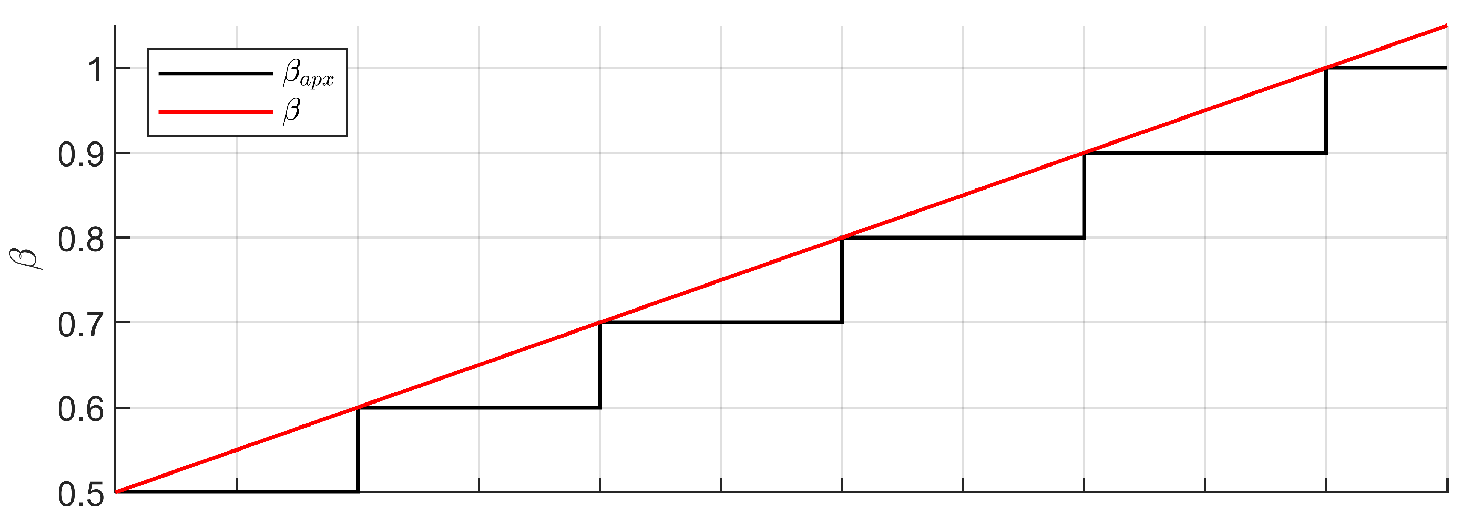
and their values were chosen according to distinct sources. Values of ${\beta }_{apx1}$ through ${\beta }_{apx6}$ are selected assuming 50% maximal controllable load reduction and, by setting adequate $\beta$ constraints ${\beta }_{max}$ and ${\beta }_{min}$, a range of values between 100 and 50 percent with 10 percent maximal rate of change $\mathsf{\Delta }{\beta }_{max}$ is achieved. It is assumed that the maintenance cost $c_{mnt}$ equals EUR 1 per hour, the shutdown cost $c{s}_{SD}$ is the same as the price of one unit of fuel and startup cost $c{s}_{SD}$ is half the shutdown cost. The natural discharge $E_{nd}$, the energy needed for storage cooling $E_{ac}$, the efficiencies ${\eta }_c$ and ${\eta }_d$ as well as the maximal amount of energy charged $\mathsf{\Delta }{E}_{s{t}_{max}}$ and discharged $\mathsf{\Delta }{E}_{s{t}_{min}}$ over $T_s$ are sourced from [27] as well as the storage capacity $E_{s{t}_{max}}$. The minimal allowed level of energy in storage $E_{s{t}_{min}}$ is selected keeping in mind that deep discharge is unacceptable. Parameters $f_a$, $f_b$ and $f_{const}$, related to fuel cost are calculated based on [34]. Generator maximum power $P_{g_{max}}$ comes from the same source. 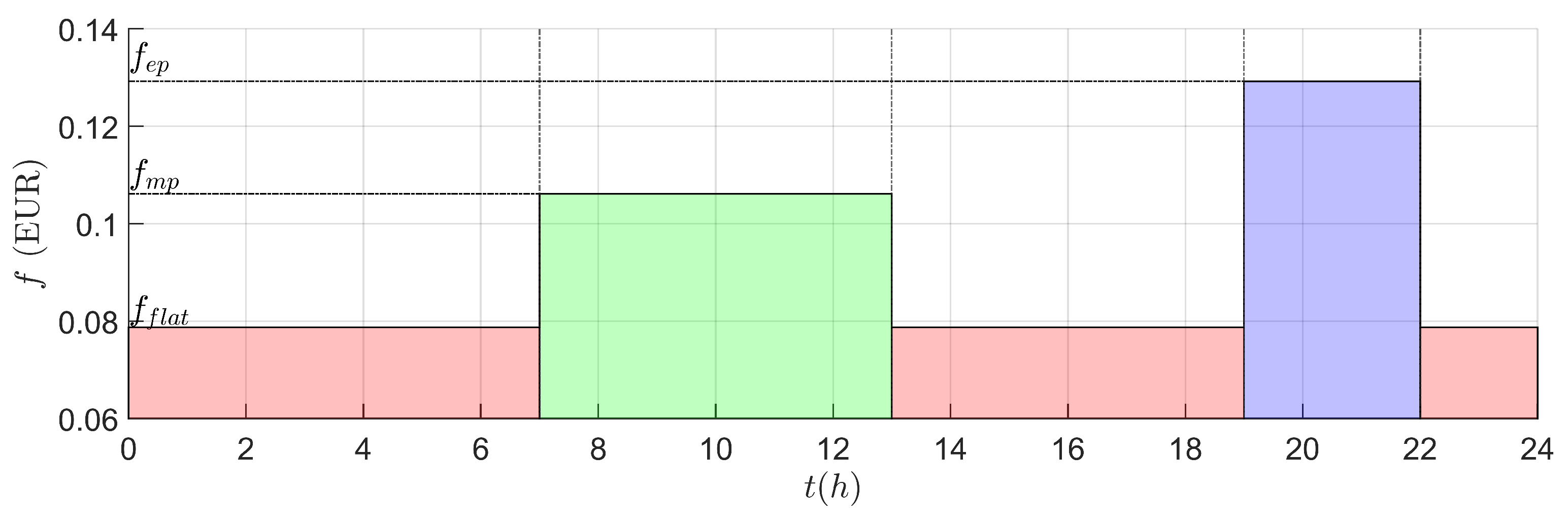Although $T_s$ may prove sufficient for the chosen generator to ramp up to full power, a much smaller additional ramp up constraint $\mathsf{\Delta }{P}_{g_{max}}$ is selected to allow for smoother operation. The energy pricing, including various fees, is borrowed from [28] and converted to euros. The generator deadband $P_{db}$, fuel threshold $P_{tr}$, required connection power $E_{e{x}_{max}}$, identical to the maximal amount of energy exchanged with public grid, sampling time $T_s$ and prediction horizon N were fine-tuned during preliminary testing.

On the other hand, matrices of weighting coefficients mentioned in Equation (47), as well as weighting matrices $R_s$ and $Q_s$ associated with single hybrid MPC used during simulation as a reference, have the following values:

$$\begin{array}{c}\hfill \begin{array}{cc}\hfill R_{on}& =\left[\begin{array}{ccc}25& 0& 0\\ 0& 50& 0\\ 0& 0& 0.1\end{array}\right]Q_{on}=\left[\begin{array}{cccccc}250& 0& 0& 0& 0& 0\\ 0& 250& 0& 0& 0& 0\\ 0& 0& 1000& 0& 0& 0\\ 0& 0& 0& 2000& 0& 0\\ 0& 0& 0& 0& 15& 0\\ 0& 0& 0& 0& 0& 5\end{array}\right]\hfill \\ \hfill R_{off}& =\left[\begin{array}{ccc}50& 0& 0\\ 0& 25& 0\\ 0& 0& 0.1\end{array}\right]Q_{off}=\left[\begin{array}{cccccc}250& 0& 0& 0& 0& 0\\ 0& 250& 0& 0& 0& 0\\ 0& 0& 100& 0& 0& 0\\ 0& 0& 0& 1& 0& 0\\ 0& 0& 0& 0& 15& 0\\ 0& 0& 0& 0& 0& 1\end{array}\right]\hfill \\ \hfill R_s& =\left[\begin{array}{ccc}25& 0& 0\\ 0& 50& 0\\ 0& 0& 0.1\end{array}\right]Q_s=\left[\begin{array}{cccccc}250& 0& 0& 0& 0& 0\\ 0& 250& 0& 0& 0& 0\\ 0& 0& 1000& 0& 0& 0\\ 0& 0& 0& 2000& 0& 0\\ 0& 0& 0& 0& 15& 0\\ 0& 0& 0& 0& 0& 3\end{array}\right]\hfill \end{array}\end{array}$$

(51)

Note that matrices dedicated to different operation modes have slightly different values. Such diversity allows for different control policies depending on connection status. For example, $R_{on}$ features a lower energy exchange penalty and much higher generator usage punishment compared to $R_{off}$. Moreover, in the case of $R_{off}$, those priorities are reversed, which is much needed in off-grid mode. On the other hand, values of $Q_s$ and $R_s$ should be viewed as a necessary compromise to accommodate for the lack of a switching mechanism. Given the fact, that on-grid mode poses more cost reduction opportunities, penalties expressed through both $Q_{on}$ and $Q_s$ encourage the management system to sell more energy if possible and buy less of it from the public grid. At the same time, $Q_{off}$ and $Q_s$ allow for a greater extent of load shedding compared to $Q_{on}$. Similarly, three reference values vectors are specified:

$$\begin{array}{c}\hfill \begin{array}{cc}\hfill y_{ron}& ={\left[\begin{array}{cccccc}0& 0& 10& 0& 90& 0\end{array}\right]}^{⊺}\hfill \\ \hfill y_{roff}& ={\left[\begin{array}{cccccc}0& 0& 0& 0& 40& 0\end{array}\right]}^{⊺}\hfill \\ \hfill y_{rs}& ={\left[\begin{array}{cccccc}0& 0& 10& 0& 65& 0\end{array}\right]}^{⊺}\hfill \end{array}\end{array}$$

(52)

All outputs except for $c_s$ and $SOC$ are to be minimized in the on-grid scenario, hence their reference values are set to zeros, which nullifies the reference value. On the other hand, $c_s$ denotes income from energy selling, therefore it is to be maximized by means of setting very high desired income and therefore turning a resulting problem into income maximization. When it comes to $SOC$, the reference value is introduced to encourage storage unit charging with renewable energy but, at the same time, to leave a sufficient margin. There is no energy sales opportunity in off-grid mode therefore, reference vector $y_{roff}$, aside from storage state of charge reference, differs only in $c_s$ reference value being changed to zero. Significantly lower target stored energy level allows to not overuse diesel generator. Values of $y_{rs}$ are similar to $y_{ron}$ with one exception being the lower state of charge reference required to achieve acceptable storage utilization in both on-grid and off-grid mode.

4.2. Simulated Microgrid Configuration

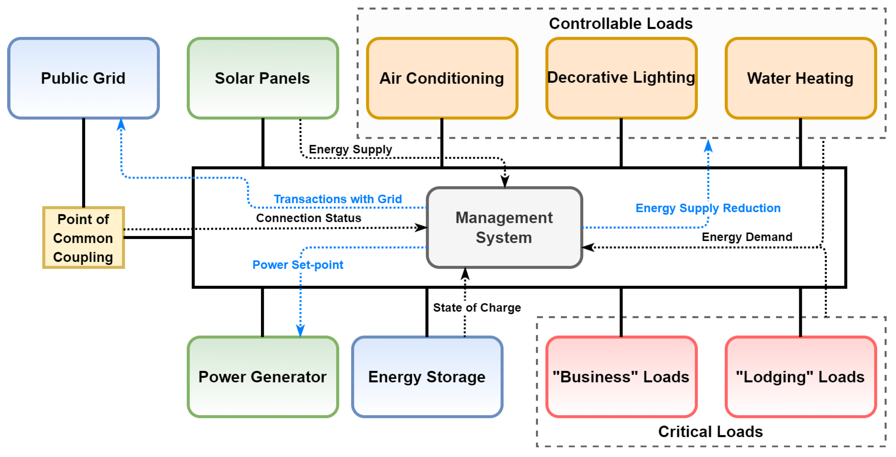
The authors choose to analyse the performance of the proposed solution when applied to a large commercial facility with its own photovoltaic installation, power generator and energy storage. This is why the aggregated, total critical energy demand profile consists of various load profiles sourced from small and medium businesses as well as residential buildings, to imitate shops, workshops, public buildings, and lodging facilities connected to the considered microgrid. Figure 4 features the structure of the analysed microgrid.

What is more, basic controllable loads are also present in form of air conditioning, water heating, and decorative elements. The microgrid is connected to the public grid via the point of common coupling and energy can be exchanged in both directions. Fundamental information flow concerning the energy management system is also shown in Figure 4. Aside from energy supply and demand, information on the connection status, as well as, the storage state is delivered to the management algorithm, while the amount of energy exchanged with the public grid, generator power set-point, and degree of energy supply reduction is returned. The main optimization goal is to minimize operation cost, but it simultaneously takes into account some technical aspects such as generator and storage usage or continuity of energy supply. Still, the system is also intended to improve the use of renewable energy. Another point is that, in off-grid mode, microgrid is unable to exchange energy with the public grid but is able to utilize excessive energy. Nevertheless, such a surplus of energy is to be avoided. On the other hand, in on-grid mode, the microgrid can freely exchange energy with the public grid. It is also worth adding that switching from on-grid to off-grid mode can be also equated with a power outage in the public grid.

4.3. Energy Generation and Demand Scenarios

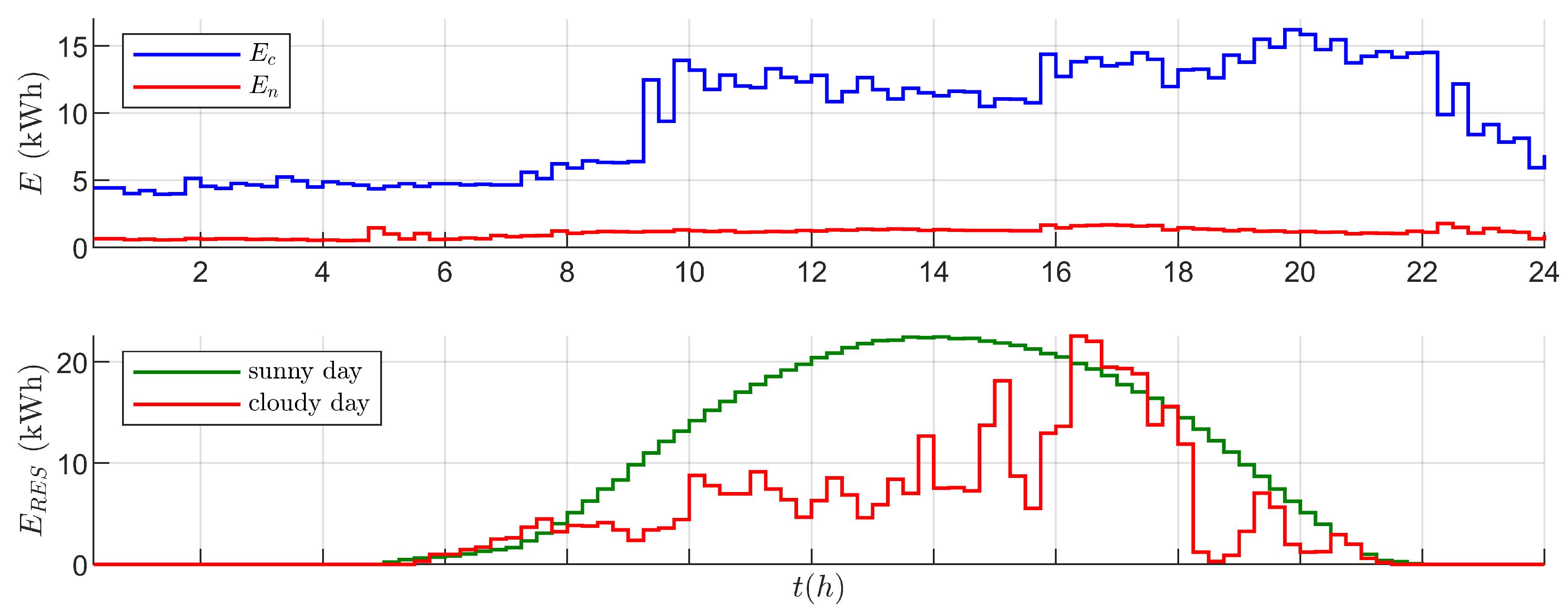
It is decided that the developed system will be tested using two solar power generation patterns, the first being a sunny day with nearly peak power and the second being a cloudy day with very changeable power output. By choosing such scenarios, the solution could be checked for economical benefits, storage level consistency, and solar energy utilisation in radically different renewable energy supply conditions. Both one-day scenarios are prepared using averaged data acquired from a solar plant located in Stargard in Poland. On the other hand, critical and non-critical demand profiles, already mentioned in the previous subsection, are prepared using end-user data sourced from [35]. Scenarios chosen for later use in the simulation are shown in Figure 5.

What is more, the total energy demand of controllable loads is fairly constant. However, critical demand is notably higher between the hours of 9:00 and 22:00.

4.4. Performed Tests and Their Methodology

Having all the necessary data, the authors opted for three-stage testing. Firstly, a basic comparison of switched HMPC performance during the sunny and the cloudy day is made. Naturally, to activate the control law switch, microgrid grid-connection mode changes during the simulation period. Such a simple method is chosen to assess how different generation scenarios affect performance in combined on-grid and off-grid operations.

Secondly, it was considered appropriate to compare the performance of the proposed approach against a standard, single, non-switched HMPC solution. Such conduct allows for a confrontation of switched MPC approach with non-switched one without additional factors and under the same conditions. As a result, the main part of the testing process is focused on evaluating the advantages and disadvantages of switched control applied to the specific case. It is mainly through the lens of economical performance but other factors, including technical aspects, are also analysed. Consequently, two types of tests have been performed at this stage:

• comparison of both control strategies over 48-h long simulation period consisting of the sunny day followed by the cloudy day and with two connection mode switches
• comparison of total operation cost for both approaches using aforementioned renewable energy supply scenario but with varying initial storage state of charge $SOC\left(0\right)$ and time of connection mode switch from on-grid to off-grid $t_{off}$.

The first routine allows for closer inspection of how individual variables change over time and how high are output values associated with economical performance. The second one is solely dedicated to total operation cost exploration in respect to a varying initial state of charge and mode-switch time. Notably, this routine consists of combined data collected from 49 individual, 48-h long, test runs. Therefore, each time, two parallel simulations were performed. Figure 6 illustrates how the tests concerning switched and non-switched HMPC were performed in MATLAB.

Following initial conditions were used during all three stages of testing:

$$\begin{array}{cc}\hfill x\left(0\right)& ={\left[\begin{array}{cccccccccccc}SOC\left(0\right)E_{s{t}_{max}}& 0& 0& 0& 0& 0& 0& 0& 0& 0& 0& 1\end{array}\right]}^{⊺}\hfill \end{array}$$

(53)

$$\begin{array}{cc}\hfill u\left(0\right)& ={\left[\begin{array}{ccc}0& 0& 100\end{array}\right]}^{⊺}\hfill \end{array}$$

(54)

The value of $SOC\left(0\right)$ is constant for the first, as well as for the second test and equals 52%. For the purposes of the third routine, two sets are defined in the following way:

$$\begin{array}{cc}\hfill \mathcal{X}& =\left\{\begin{array}{ccccccc}30& 40& 50& 60& 70& 80& 90\end{array}\right\}\hfill \end{array}$$

(55)

$$\begin{array}{cc}\hfill \mathcal{S}& =\left\{\begin{array}{ccccccc}0& 8& 16& 24& 32& 40& 48\end{array}\right\}\hfill \end{array}$$

(56)

as well as their Cartesian product:

$$\mathcal{XS}=\mathcal{X}\times \mathcal{S}$$

(57)

The set $\mathcal{X}$ contains percentage $SOC\left(0\right)$ values, and the set $\mathcal{S}$ contains connection mode switch times $t_{off}$. The set $\mathcal{XS}$ contains all ordered pairs from sets $\mathcal{X}$ and $\mathcal{S}$.

As a result, for each of the 49 pairs test runs are performed using every combination of initial states of charge $SOC\left(0\right)$ and mode change times $t_{off}$ contained in the table $\mathcal{XS}$. It is also worth adding that in this case, only one operation mode switch happens during the simulation and the microgrid always starts in on-grid mode.

5. Results

Having hybrid microgrid model, control laws, and all the parameters, as well as data, prepared, simulations are carried over. In order to properly analyse the results, measures of performance are introduced. Summary startup and shutdown, maintenance, and energy costs, as well as income from selling energy, are used to better understand simulation results. Moreover, average $SOC$ and $\beta$ are also analysed. All those values are presented in appropriate tables. Furthermore, corresponding figures containing storage state of charge, energy balance, and all system inputs are also provided. The comments concerning the first two testing routines are made based on information derived from relevant figure-table pairs. The last routine is discussed on the basis of the appropriate figure, as well as some additional numerical data.

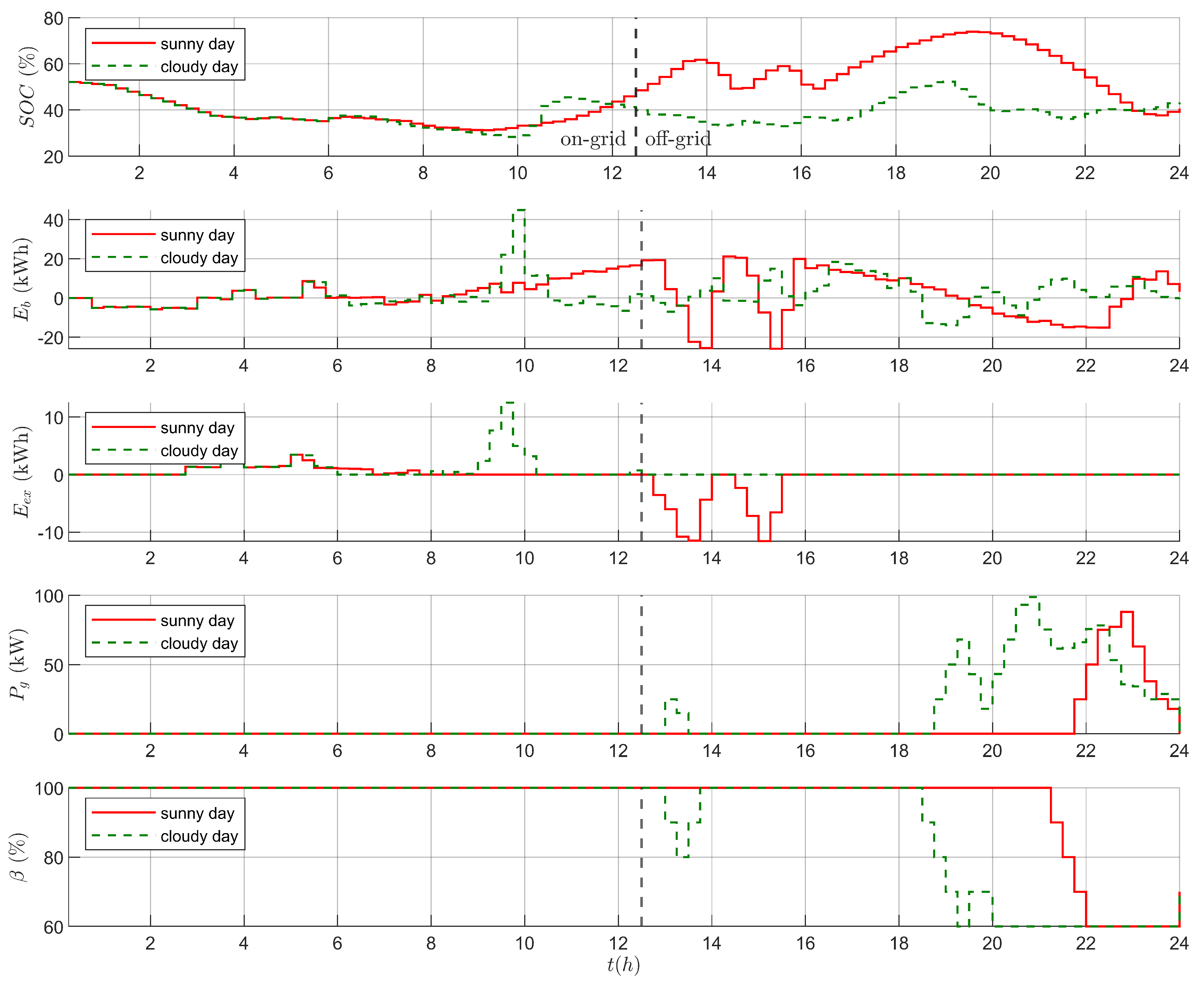
5.1. Comparison of Microgrid Performance in Different Renewable Energy Generation Scenarios

The numerical results obtained from sunny and cloudy renewable energy generation scenarios analysis are summarised in

Table 2. Aggregated output values associated with microgrid operation cost and averaged state of charge and energy demand reduction coefficient values for sunny and cloudy day.

Variable	Sunny Day	Cloudy Day	Unit
$C_{st}=\sum c_{st}$	0.89	2.24	EUR
$C_{mg}=\sum c_{mg}$	32.43	82.41	EUR
$C_s=\sum c_s$	0	0	EUR
$C_b=\sum c_b$	8.77	19.04	EUR
$C_{total}=\sum (c_{st}+c_{mg}-c_s+c_b)$	42.09	103.69	EUR
$\overline{SOC}$	47.60	38.84	%
$\overline{\beta }$	95.73	90.94	%

, while Figure 7 compares storage state of charge, energy balance, and system inputs over the simulation horizon. It is apparent from the aforementioned table that the cloudy day turned out to be significantly more costly. For instance, $C_{st}$, $C_{mg}$, and $C_b$ have, respectively, about 2.5, 2.5, and 2.2 times higher values for the case of the cloudy day in comparison to the case of the sunny day. Consequently, this leads to a 146% higher total operation cost. As Figure 7 shows, such a huge difference stems from the necessity of compensating for lacking energy supply in off-grid mode, mainly after 18:00, by means of the power generator. In contrast, higher SOC in the evening of the sunny day translates into a longer period without the need for energy generated from diesel fuel.

From the chart, it can be also seen that SOC in on-grid mode is kept relatively low in wait for renewable energy supply but when a significant amount of energy becomes available operation mode is changed. In both scenarios, storage is charged visibly over the level specified by the reference value, but in the case of the cloudy day, this process is much less significant. That explains why the average $\overline{SOC}$ during the cloudy day is 18% lower. Given the limited time in on-grid mode, there is no energy being sold regardless of the scenario, hence $C_s$ equals zero. Additionally, in Figure 7 there is a clear trend of reducing controllable load energy supply only when diesel generator is needed. It can be also seen from the aforementioned figure, that more fluctuations of energy balance ($E_b$) occur in off-grid mode. Furthermore, around 14:00 during the sunny day, a significant amount of excess energy appears.

It is important to emphasize that the purpose of this test is to initially verify if chosen modeling and control approach is appropriate and combined lead to satisfactory results in one of the simpler scenarios. Summarizing, performed test exhibited that chosen switched control approach is capable of handling basic energy generation and grid-connection scenarios. It proves able to use the capacity of the storage to its advantage and to not overuse power generator although some excess energy occurred, which is not ideal.

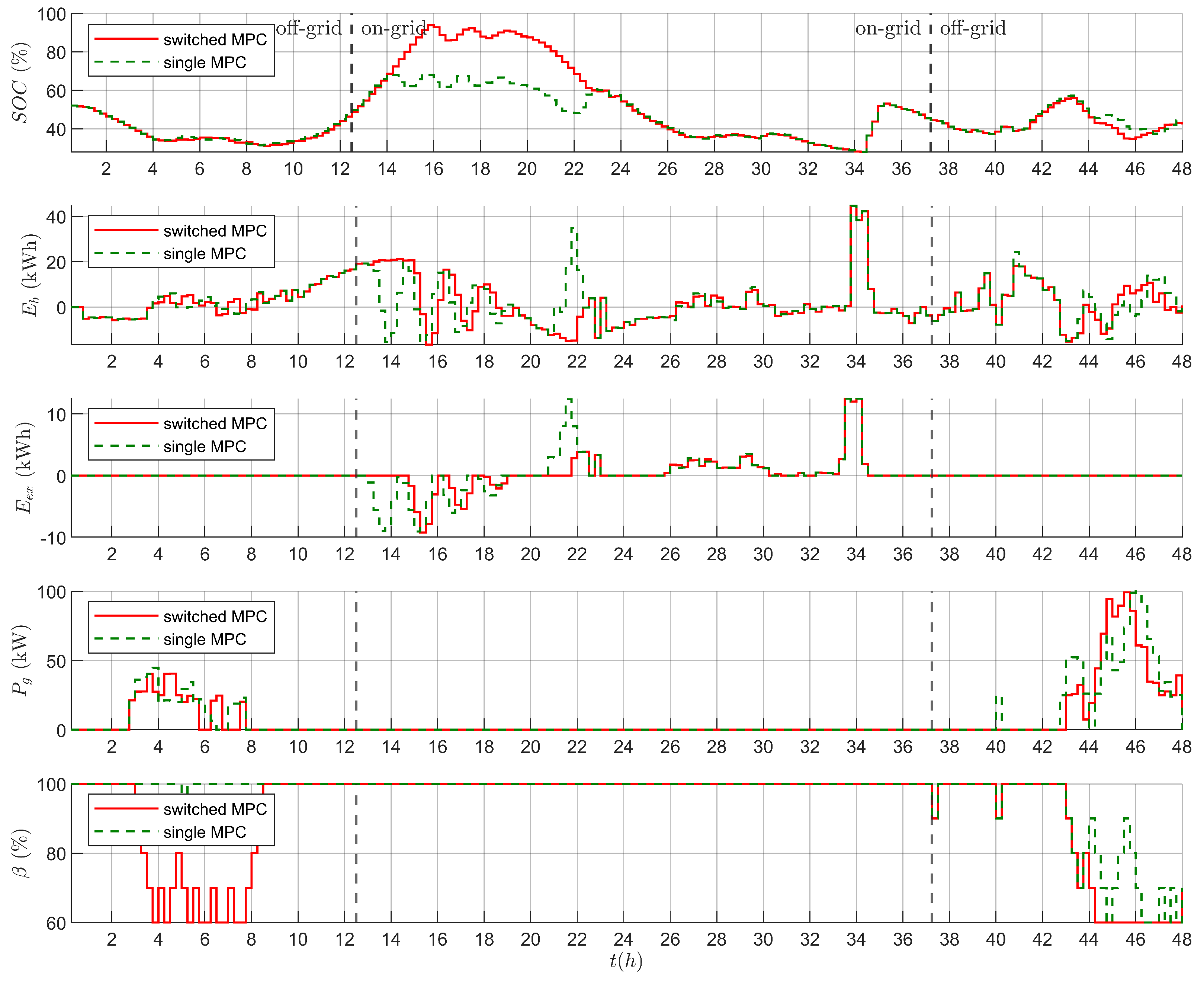
5.2. Comparison of Microgrid Performance Using Switched and Non-Switched HMPC Control

Turning now to the second test, the developed switched HMPC approach is compared with standard, single hybrid MPC. The analysis is based on a 48-h long simulation including both the sunny and cloudy days, as well as two grid-connection mode transitions. The numerical data produced as a result are gathered in

Table 3. Aggregated output values associated with microgrid operation cost and averaged state of charge and energy demand reduction coefficient values obtained using switched and single hybrid MPC solutions in the two-day scenario.

Variable	Switched HMPC	Single HMPC	Unit
$C_{st}=\sum c_{st}$	4.93	4.93	EUR
$C_{mg}=\sum c_{mg}$	99.81	112.06	EUR
$C_s=\sum c_s$	10.83	18.16	EUR
$C_b=\sum c_b$	30.28	40.55	EUR
$C_{total}=\sum (c_{st}+c_{mg}-c_s+c_b)$	124.19	139.38	EUR
$\overline{SOC}$	48.62	45.09	%
$\overline{\beta }$	92.50	96.82	%

and matching charts are presented in Figure 8. Firstly, as Table 3 shows, $C_{mg}$ and $C_b$ are higher for the case of single hybrid MPC by about 12% and 34%, respectively. This denotes that, although $P_g$ charts for both cases seem similar, single HMPC tend to use the generator to a slightly greater extent. What is more, switched HMPC tend to buy significantly less energy in the on-grid mode based on data contained in Figure 8. Besides, there is no excess energy at all in off-grid mode, regardless of the control approach and both control laws make the grid sell a substantial amount of energy.

Interestingly enough, as presented in Table 3, a single HMPC manages to achieve 67% greater income from energy sales compared to the competitive solution but its summary operation cost is higher by about 12%. This leads to the conclusion that overall energy exchange with the public grid is more efficient in the case of switched HMPC, especially considering identical $C_{st}$ values and similar $P_g$ values over the whole simulation period. Another point is that switched solution also provides 8% higher average state of charge (calculated as percent relative difference). Figure 8 illustrates that both solutions exhibit similar trends in respect of SOC, although, considering $E_b$ and $\overline{SOC}$, switched approach seem to provide a slightly more consistent storage energy level than the single MPC solution. This can prove important when considering the storage life cycle. Nevertheless, the single MPC provides 5% higher average $\beta$ value even though it features a greater extent of load shedding penalization. Still, the share of the controllable load in overall energy demand is relatively small and it does not translate into significant gains in economical terms. Admittedly, the performed test shows that switched HMPC approach has a slight advantage over single HMPC control not just in terms of economical benefits.

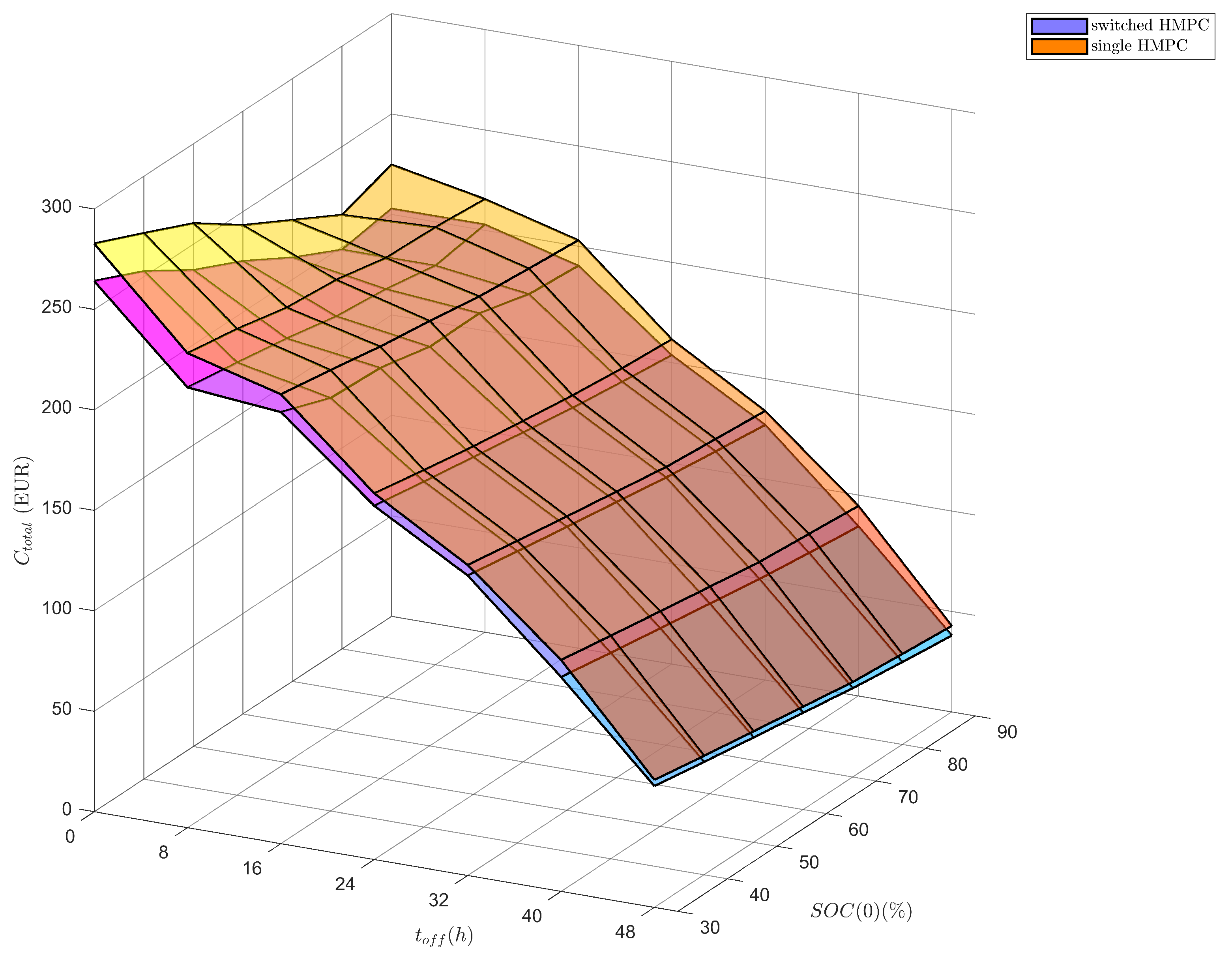
5.3. Comparison of Switched and Non-Switched HMPC Control Performance in Various Connection Scenarios and with Varying Initial Storage State of Charge

The previous test shows the advantage of switched hybrid MPC on the example of a single scenario but it falls short in proving its superiority in a wider variety of circumstances. Therefore, to somehow address obvious concerns about the adequacy of the proposed solution third testing routine is introduced. Through preliminary testing, the initial state of charge $SOC\left(0\right)$ and the time of the transition between on-grid and off-grid operation $t_{off}$ are selected as key factors with possibly the biggest impact on simulation results. Finally, as mentioned in the previous section, 49 simulations covering various combinations of $SOC\left(0\right)$ and $t_{off}$ are conducted, and gathered data is used to create surfaces shown in Figure 9.

Although the third testing procedure is the most complicated one, conclusions based on the relation of both surfaces are rather simple. As it turns out, the quantity of time in different operation modes has the biggest impact on total microgrid operation cost, while the impact of the initial state of charge is rather marginal. The single most striking observation to emerge from overall cost comparison is the fact, that the cost-surfaces do not intersect and the surface related to switched hybrid MPC is located below the surface tied to the single HMPC, which in turn, proves that in all 49 cases, overall operation cost is lower when utilizing the novel solution proposed by the authors. The greater the share of off-grid operation, the more significant the gains become, which may seem obvious considering two oriented on specific mode cost functions as opposed to only one. Averaged total operation cost reduction amounts to 6.26% when using switched MPC with a maximal cost reduction of 11.23% and a minimal reduction of 3.12%, which proves the adequacy of the proposed method based on simulation data available to the authors.

6. Conclusions

Research presented in this paper led to the development of a microgrid economical optimization strategy based on switched hybrid model predictive control as well as a compatible microgrid hybrid model on the basis of which the receding horizon control algorithm operates. The performance of the proposed control scheme was analyzed through three-stage simulation testing using real solar generation data and real energy demand profiles. The study was intended to compare and contrast the level of performance gains offered by switched model predictive control compared to non-switched one. The introduced solution proved to be effective in changing grid connection conditions and renewable energy generation regardless of the grid-connection scenario. Its usage led to a 6% averaged total operation cost reduction in comparison with the single HMPC strategy. Another important point is that the greater the share of off-grid operation, the more significant the gains become. Besides, this profit is made mainly due to better renewable energy utilisation management. An obvious drawback is the lack of means of energy demand and production forecasting, which means optimization is performed assuming constant demand and production over the prediction horizon. This is not ideal but, given the fact that the system presented in this paper manages to work well without forecasting certain data, this approach can be deemed useful for simple systems. Nonetheless, implementing such functionalities could noticeably improve performance.

Despite needing minor amendments, the proposed solution can be used in microgrid management systems intended to cope with common energy supply interruptions or highly autonomous microgrids in remote regions. Due to generalized microgrid model formulation and commonly available and exchangeable tools, the proposed model and control scheme does not depend on specific equipment or software and should be applicable to any standard microgrid. Given the conceptual character of this study, the authors intend to supplement more functionalities through further research and address shortcomings found during testing. Future work suggests the implementation of advanced energy demand and supply forecasting capabilities, as well as more sophisticated demand-side management functionalities.

References

1. Garcia-Torres, F.; Zafra-Cabeza, A.; Silva, C.; Grieu, S.; Darure, T.; Estanqueiro, A. Model Predictive Control for Microgrid Functionalities: Review and Future Challenges. Energies 2021, 14, 1296. [Google Scholar] [CrossRef]
2. Bordons, C.; Garcia-Torres, F.; Ridao, M.A. Model Predictive Control of Microgrids; Springer Nature: Cham, Switzerland, 2020. [Google Scholar] [CrossRef]
3. Hu, J.; Shan, Y.; Guerrero, J.; Ioinovici, A.; Chan, K.; Rodriguez, J. Model predictive control of microgrids—An overview. Renew. Sustain. Energy Rev. 2020, 136, 110422. [Google Scholar] [CrossRef]
4. Topa Gavilema, A.O.; Alvarez, J.D.; Torres Moreno, J.L.; Garcia, M.P. Towards Optimal Management in Microgrids: An Overview. Energies 2021, 14, 5202. [Google Scholar] [CrossRef]
5. Ahmad, S.; Ullah, I.; Jamil, F.; Kim, D. Toward the Optimal Operation of Hybrid Renewable Energy Resources in Microgrids. Energies 2020, 13, 5482. [Google Scholar] [CrossRef]
6. Zhang, X.; Wang, Z.; Lu, Z. Multi-objective load dispatch for microgrid with electric vehicles using modified gravitational search and particle swarm optimization algorithm. Appl. Energy 2022, 306, 118018. [Google Scholar] [CrossRef]
7. Yang, Y.; Qiu, J.; Qin, Z. Multidimensional Firefly Algorithm for Solving Day-Ahead Scheduling Optimization in Microgrid. J. Electr. Eng. Technol. 2021, 16, 1755–1768. [Google Scholar] [CrossRef]
8. Kim, R.K.; Glick, M.B.; Olson, K.R.; Kim, Y.S. MILP-PSO Combined Optimization Algorithm for an Islanded Microgrid Scheduling with Detailed Battery ESS Efficiency Model and Policy Considerations. Energies 2020, 13, 1898. [Google Scholar] [CrossRef] [Green Version]
9. Wang, L.; Xue, A. Equivalent Modeling of Microgrids Based on Optimized Broad Learning System. Energies 2021, 14, 7911. [Google Scholar] [CrossRef]
10. Lopez-Garcia, T.B.; Coronado-Mendoza, A.; Domínguez-Navarro, J.A. Artificial neural networks in microgrids: A review. Eng. Appl. Artif. Intell. 2020, 95, 103894. [Google Scholar] [CrossRef]
11. Abdolrasol, M.G.M.; Mohamed, R.; Hannan, M.A.; Al-Shetwi, A.Q.; Mansor, M.; Blaabjerg, F. Artificial Neural Network Based Particle Swarm Optimization for Microgrid Optimal Energy Scheduling. IEEE Trans. Power Electron. 2021, 36, 12151–12157. [Google Scholar] [CrossRef]
12. Otani, T.; Tanabe, R.; Koyanagi, Y.; Iwamoto, S. Cooperative load frequency control of generator and battery using a recurrent neural network. In Proceedings of the TENCON 2017—2017 IEEE Region 10 Conference, Penang, Malaysia, 5–8 November 2017; pp. 918–923. [Google Scholar] [CrossRef]
13. Hamedi, K.; Sadeghi, S.; Esfandi, S.; Azimian, M.; Golmohamadi, H. Eco-Emission Analysis of Multi-Carrier Microgrid Integrated with Compressed Air and Power-to-Gas Energy Storage Technologies. Sustainability 2021, 13, 4681. [Google Scholar] [CrossRef]
14. Yang, J.; Su, C. Robust optimization of microgrid based on renewable distributed power generation and load demand uncertainty. Energy 2021, 223, 120043. [Google Scholar] [CrossRef]
15. Silva, J.A.A.; Lopez, J.C.; Arias, N.B.; Rider, M.J.; da Silva, L.C.P. An optimal stochastic energy management system for resilient microgrids. Appl. Energy 2021, 300, 117435. [Google Scholar] [CrossRef]
16. Rezaei, N.; Khazali, A.; Mazidi, M.; Ahmadi, A. Economic energy and reserve management of renewable-based microgrids in the presence of electric vehicle aggregators: A robust optimization approach. Energy 2020, 201, 117629. [Google Scholar] [CrossRef]
17. Mosa, M.A.; Ali, A.A. Energy management system of low voltage dc microgrid using mixed-integer nonlinear programing and a global optimization technique. Electr. Power Syst. Res. 2021, 192, 106971. [Google Scholar] [CrossRef]
18. Alhumaid, Y.; Khan, K.; Alismail, F.; Khalid, M. Multi-Input Nonlinear Programming Based Deterministic Optimization Framework for Evaluating Microgrids with Optimal Renewable-Storage Energy Mix. Sustainability 2021, 13, 5878. [Google Scholar] [CrossRef]
19. Borrelli, F.; Bemporad, A.; Morari, M. Predictive Control for Linear and Hybrid Systems; Cambridge University Press: Cambridge, UK, 2017. [Google Scholar] [CrossRef] [Green Version]
20. Tatjewski, P. Advanced Control of Industrial Processes: Structures and Algorithms; Advances in Industrial Control; Springer: London, UK, 2007. [Google Scholar] [CrossRef]
21. Parisio, A.; Rikos, E.; Glielmo, L. A Model Predictive Control Approach to Microgrid Operation Optimization. IEEE Trans. Control Syst. Technol. 2014, 22, 1813–1827. [Google Scholar] [CrossRef]
22. Conte, E.; Mendes, P.R.C.; Normey-Rico, J.E. Economic Management Based on Hybrid MPC for Microgrids: A Brazilian Energy Market Solution. Energies 2020, 13, 3508. [Google Scholar] [CrossRef]
23. Khakimova, A.; Shamshimova, A.; Sharipova, D.; Kusatayeva, A.; Ten, V.; Bemporad, A.; Familiant, Y.; Shintemirov, A.; Rubagotti, M. Hybrid model predictive control for optimal energy management of a smart house. In Proceedings of the 2015 IEEE 15th International Conference on Environment and Electrical Engineering (EEEIC), Rome, Italy, 10–13 June 2015; pp. 513–518. [Google Scholar] [CrossRef]
24. Paula e Silva, D.; Salles, J.; Fardin, J.; Pereira, M. Management of an island and grid-connected microgrid using hybrid economic model predictive control with weather data. Appl. Energy 2020, 278, 115581. [Google Scholar] [CrossRef]
25. Olama, A.; Mendes, P.R.; Camacho, E.F. Lyapunov-based hybrid model predictive control for energy management of microgrids. IET Gener. Transm. Distrib. 2018, 12, 5770–5780. [Google Scholar] [CrossRef]
26. Dou, C.; Zhou, X.; Zhang, T.; Xu, S. Economic Optimization Dispatching Strategy of Microgrid for Promoting Photoelectric Consumption Considering Cogeneration and Demand Response. J. Mod. Power Syst. Clean Energy 2020, 8, 557–563. [Google Scholar] [CrossRef]
27. Saft Batteries. Intensium® Mini Flexible Lithium-Ion Energy Storage System Datasheet. Available online: https://cdn.enfsolar.com/Product/pdf/storage_system/5a41f616848ec.pdf (accessed on 10 July 2021).
28. ENEA S. A. ENEA Energy Tariff 2021. Available online: https://www.enea.pl/dlafirm/obsluga_klienta_i_kontakt/2021/enea_operator_taryfa_2021.pdf (accessed on 10 July 2021).
29. Polish Energy Regulatory Office. Average Sales Price on Polish Competitive Energy Market (Annual and Quarterly). Available online: https://www.ure.gov.pl/pl/energia-elektryczna/ceny-wskazniki/7852,Srednia-cena-sprzedazy-energii-elektrycznej-na-rynku-konkurencyjnym-roczna-i-kwa.html (accessed on 10 July 2021).
30. Torrisi, F.; Bemporad, A. HYSDEL-a tool for generating computational hybrid models for analysis and synthesis problems. IEEE Trans. Control Syst. Technol. 2004, 12, 235–249. [Google Scholar] [CrossRef]
31. Bemporad, A.; Morari, M. Control of systems integrating logic, dynamics, and constraints. Automatica 1999, 35, 407–427. [Google Scholar] [CrossRef]
32. Herceg, M.; Kvasnica, M.; Jones, C.N.; Morari, M. Multi-Parametric Toolbox 3.0. In Proceedings of the IEEE 2013 European Control Conference (ECC), Zurich, Switzerland, 17–19 July 2013; pp. 502–510. [Google Scholar] [CrossRef] [Green Version]
33. Gurobi Optimization LLC. Gurobi—The Fastest Solver. Available online: https://www.gurobi.com/ (accessed on 16 December 2021).
34. Proton Polska. Proton ZPP 100 Energy Generator Datasheet. Available online: https://proton-polska.pl/product-pol-525-Agregat-pradotworczy-Proton-ZPP-100-100kW-110kW.html (accessed on 16 December 2021).
35. Customer-Led Network Revolution. Customer-Led Network Revolution Dataset. Available online: http://www.networkrevolution.co.uk/resources/project-data/ (accessed on 16 December 2021).
Figure 1. Energy price chart according to chosen energy tariff.
Energies 15 00833 g001
Figure 2. Visualization of β approximation.
Energies 15 00833 g002
Figure 3. Schematic diagram of the chosen control system structure with switching between two hybrid model predictive control laws.
Energies 15 00833 g003
Figure 4. Considered microgrid configuration for a large commercial facility.
Energies 15 00833 g004
Figure 5. Critical and non-critical energy demand and solar energy data used during simulation.
Energies 15 00833 g005
Figure 6. Diagram showing the methodology used to compare switched and non-switched HMPC performance.
Energies 15 00833 g006
Figure 7. Storage state of charge, energy balance and all system inputs over a 24-h simulation period of the sunny and cloudy day.
Energies 15 00833 g007
Figure 8. Storage state of charge, energy balance, and all system inputs obtained using switched and single hybrid MPC solutions in the two-day scenario.
Energies 15 00833 g008
Figure 9. The total cost of microgrid operation depends on the initial storage state of charge and the time at which operation mode is changed from on-grid to off-grid.
Energies 15 00833 g009