Abstract
Multi-energy systems (MES) allow various energy forms, such as electricity, gas, and heat, to interact and achieve energy transfer and mutually benefit, reducing the probability of load cutting in the event of a failure, increasing the energy utilization efficiency, and improving the reliability and robustness of the overall energy supply system. Since energy storage systems can help to restore power in the case of failure and store the surplus energy to enhance the flexibility of MES, this work provides a methodology for reliability optimization, considering different energy storage configuration schemes under weather uncertainties. First of all, a reliability evaluation model of a multi-energy system under weather uncertainties based on a sequential Monte Carlo simulation is established. Then, the reliability optimization problem is formulated as a multi-objective optimization problem to minimize the reliability index, SAIDI (system average interruption duration index), and the reliability cost. Finally, a case study implemented on a typical MES layout is used to demonstrate the proposed methodology. A comparative analysis of three widely adopted multi-objective metaheuristic algorithms, including NSGA-II (non-dominated sorting genetic algorithm II), MOPSO (multiple objective particle swarm optimization), and SPEA2 (strength Pareto evolution algorithm 2), is performed to validate the effectiveness of the proposed method. The simulation results show that the NSGA-II algorithm leads to better optimal values and converges the fastest compared to the other two methods.
1. Introduction
Multi-energy systems refer to a new, unified view of energy systems formed by the coupling of cooling and heating in gas and electricity supplies during the transmission and distribution processes, which has the potential to make energy monitoring, generation, consumption, and maintenance more efficient. Multi-energy systems can take full advantage of the interaction between various forms of energy sources to improve system economics, increase system flexibility, and enhance system reliability. However, due to the complex structure of MES and the enormous components they contain, the failure of a single component could have a significant impact on a multi-energy system’s overall operation. Thus, it is critical to assess and improve MES reliability effectively and accurately. Multi-energy system reliability is defined as the extent to which the performance of the components in a bulk system provides the customer with electrical, thermal, and gas energy within agreed criteria [1]. Besides assessing MES reliability, improving it is also essential, as it can enhance MES stability and provide energy to the customers more efficiently [2]. MES reliability can be improved by enhancing its flexibility through the optimized use of energy storage systems, which can compensate for the volatility and the uncertainty of renewable generation, such as wind and PV power generation. Therefore, this study explores how to optimize the energy storage configuration schemes to optimize MES reliability.
1.1. MES Reliability Assessment Overview
After Roy Billiton introduced reliability assessment analysis [3], a large number of researchers conducted multi-energy system reliability assessments. The vast majority of studies focus on the single coupling system, mainly on electricity and heat, with specific application areas [4]. In Ref. [2], the reliability assessment of an electricity–heat integrated energy system with heat pumps based on a Monte Carlo simulation is proposed. The effects of the CCHP system on energy supply reliability are analyzed in [5], concluding that combining energy supplies can significantly increase overall system reliability. In [6,7], the natural gas network combined with the power distribution system is modeled for the reliability evaluation. A few studies of power–gas–heat multi-energy systems have been undertaken, based on the reliability assessment of single coupling systems. The authors in [8] assess the reliability of a multi-carrier energy system with varying levels of demand while accounting for the uncertainty of different weather conditions. In [9], a user experience-based reliability evaluation of an electricity–gas–heat MES is defined and reliability indicators from the standpoint of user severity and satisfaction with energy consumption are provided. Although the studies evaluate the system reliability by integrating all of the three energy forms, and the authors in [8] also take into account the weather uncertainty, they do not include in their assessment of integrated energy systems renewable energy and energy storage systems, which are instead considered to be essential components of future sustainable energy grids. Multi-energy system reliability evaluation, considering energy storage devices, is introduced in [10,11,12]. The authors in [10] propose a multi-carrier energy system to assess MES reliability while accounting for the influence of energy storage devices. The authors in [11] propose assessing microgrid reliability with energy storage systems by utilizing a Monte Carlo simulation, which considers multi-energy coupling and grade difference. A reliability evaluation approach is devised in [12] by integrating the FMEA (failure mode and effect analysis) method and Monte Carlo simulation to analyze multi-energy micro-grids’ reliability while considering various distinct operational strategies for energy storage devices. An MES integrated with electrical vehicles, which are mobile energy storage systems, has been considered in reliability evaluation. The influence of V2G (vehicle to grid) technology on distribution system reliability is studied in [13], using the 24 h available energy model of electric vehicles. The aforementioned works [10,11,12,13] clearly show the key role storage systems play in supporting MES reliability and flexibility. Based on the findings of these studies, it is essential to consider storage systems in order to optimize MES reliability.
1.2. MES Reliability Optimization Overview
Since energy storage devices can restore power in the event of a power outage while also storing excess energy, reliability optimization that considers different energy storage configuration schemes is essential to enhance the energy supply reliability. Moreover, the primary goal of MES optimization is to satisfy the customer demand at the lowest possible cost while ensuring the highest system reliability [14]. Thus, a multi-objective method is considered in this work to optimize both system reliability and the cost of relative energy storage system investment and the energy not supplied.
Some researchers have attempted to incorporate the results of reliability evaluations into optimal planning problems based on the reliability evaluation approach. The authors in [14] use a Monte Carlo simulation and particle swarm optimization approach to develop an optimal reliability plan for a composite electric power system. The multi-objective optimization of a grid-connected PV–wind hybrid system, taking into account reliability, economic, and environmental factors, is proposed in [15]. The authors in [16] optimize residential buildings with regard to energy demand while imposing reliability constraints, without considering costs. A standalone renewable energy system for 250 households in India, considering the cost of electricity and reliability, is designed in [17]. An optimal day-ahead dispatch and model of predictive control for energy hubs is explored in [18] for simple energy hub layouts, but without considering the optimal system design. The previous research focused on either single energy system optimization or single objective optimization. The economics and reliability of multi-energy systems are still not co-optimized simultaneously, however, despite both being key aspects that need to be taken into account.
1.3. Main Contributions
Even though the studies mentioned above are relevant, there are still significant gaps and open challenges:
- The reliability assessment of multi-energy systems primarily focuses on single coupling systems, such as power–heat and power–gas systems, and assessments seldom focus on multi-energy systems that combine all three energy forms of power, heat, and natural gas;
- The established reliability modeling approach is very simplistic, ignoring component uncertainty and time-varying load in real-world situations;
- Most previous works solved the problem as a single optimization problem, with the goal of maximizing reliability or lowering cost as the sole objective, and there is still no detailed investigation of optimal storage system design for multi-energy system reliability.
To address these gaps, a sequential Monte Carlo simulation is adopted to assess and quantify MES reliability, based on well-known performance indicators (e.g., the reliability index, SAIDI), and considering storage devices and PV, as well as wind uncertainties. The Monte Carlo simulation is a mathematical technique for modeling risk or uncertainty in complex large-scale systems, and thus can help simulate their operation by using repeated random sampling from the specific probability distribution of random variables [19]. There are two types of Monte Carlo simulation: non-sequential (or random) Monte Carlo and sequential Monte Carlo (chronological). Sequential Monte Carlo simulation, as opposed to the non-sequential approach, simulates the system states in a chronological sequence. Since an MES is a large-scale, complex, dynamic system, the sequential method is more appropriate for evaluating MES reliability [20]. The Monte Carlo simulation approach is integrated into the problem of optimizing MES reliability, taking economic considerations into account. Thus, a reliability optimization is formulated as a multi-objective problem aiming to maximize MES reliability in a cost-effective manner. The resulting optimization problem is highly complex and nonconvex, with a large number of variables and strongly coupled subsystems. Because of this, solving such an optimization problem using analytical methods, such as interior point and branch-and-bound methods, is extremely hard, and metaheuristics are a more suitable option [21]. Metaheuristic methods, such as genetic algorithms and particle swarm optimization, are widely utilized in the energy system domain to tackle numerous problems [21], which include reliability optimization, economic dispatch, optimal power flow, distribution system reconfiguration, load and generation forecasting, and maintenance scheduling. These are solved using metaheuristic optimization in [22,23,24]. Among them, the Pareto-based MOEA (multi-objective evolutionary algorithms), including NSGA-II, MOPSO, and SPEA2, appear to be the most commonly used. The Pareto front contains a set of non-dominated solutions from which decision makers can choose their preferred one [21]. Since metaheuristics can address multiple-objective, multiple-solution problems and can calculate high-quality solutions to complicated real-world problems [25], this paper adopts these three methods—NSGA-II, SPEA2, and MOPSO to find out the optimal storage device placement schemes. NSGA-II [26], which is one of the most frequently used genetic algorithms and is based on the crowding distance criterion (the average distance between a given solution and the nearest solution belonging to the Pareto front; individuals with greater crowding distances are reserved for the next generation), has a strong capability to avoid being trapped in a local optimal solution. Moreover, NSGA-II has shown fast and efficient convergence to Pareto solutions. Unlike NSGA-II, SPEA2 [27] uses a different criterion-clustering method, which preserves the characteristics of the nondominated solutions. In high-dimensional objective spaces, SPEA2 appears to outperform NSGA-II. However, NSGA-II has a “broader range” of solutions, and is thus more likely to obtain solutions closer to the Pareto optimal front [27]. The principle and technique of MOPSO [28] are relatively simple compared to the other algorithms. MOPSO is based on the flocking behavior of birds, in which an individual’s movement is influenced by the locations and movements of nearby individuals. MOPSO also exhibits a fast convergent rate; however, it performs worse than genetic algorithms at finding Pareto solutions. Based on the different characteristics of the above algorithms, this paper employs these three algorithms to validate and compare the effectiveness of the obtained results.
The main contributions of this paper are as follows:
- The power–heat–gas multi-energy system reliability with energy storage devices has been modeled, taking into account all the coupling components under weather uncertainties;
- The uncertainty modeling of PV and wind generation and time-varying load forecasting, including heat and gas demand, are considered. Moreover, a time varying cost model based on the sector customer damage function (SCDF) [29] is also adopted to calculate the EENS (expected energy not supplied) and the interruption cost in objective functions;
- A multi-objective reliability optimization problem is formulated considering both the system reliability index, SAIDI, and costs (including interruption cost and the installation cost of multi-energy storage devices) as objective functions. The optimization results are compared through the three widely used algorithms, i.e., the particle swarm algorithm, genetic algorithm, and evolutionary algorithm, to validate the feasibility and effectiveness of the suggested approach.
2. Overall Modeling Architecture of Multi-Energy System
Figure 1 is a schematic diagram of a typical MES. The structure of a generic multi-energy system includes three main parts: the power grid (PG), heat network (HN), and gas network (GN). Besides the power generation unit PV (photovoltaic), WT (wind turbine), and three kinds of energy storage devices, ES (electricity storage), HS (heat storage), and GS (gas storage), coupling components, such as combined heat and power (CHP), power to gas (P2G), vehicle to grid (V2G), and gas boiler (GB), are also considered in the MES modeling. P2G, as a novel energy conversion technology, alters the current condition of one-way natural gas to electricity conversion through gas turbines and brings the power grid and natural gas network closer. P2G technology in the electric–gas combined network not only improves power and natural gas coupling and promotes optimal operation between multi-energy flows, but it also converts surplus wind energy into natural gas during the peak wind power season to reduce the amount of abandoned wind energy. CHP is another coupling component that can generate power and heat simultaneously. This technology can increase energy efficiency by utilizing waste heat from industrial production. The V2G system allows for two-way energy flow (charge and discharge) between the electric vehicle and the grid, alleviating grid power supply pressure and improving battery utilization efficiency.
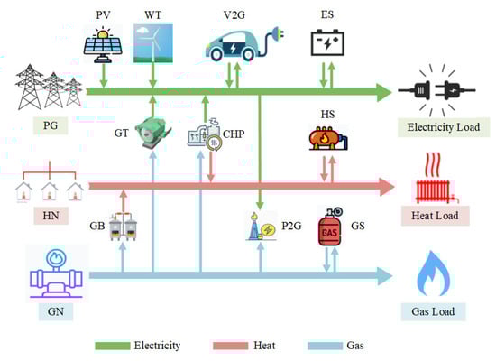
Figure 1.
The structure of MES.
2.1. Multi-Energy System Components Modeling
The various MES components will have a significant influence on the system’s overall operation. In order to assess and optimize the reliability of an MES, a mathematical model of MES components is needed, which will be illustrated in this section.
2.1.1. CHP Unit
The CHP (combined heat and power) unit includes power production, heat production, and gas consumption. During the time period t, the amount of natural gas consumed by CHP is [30]:
where is the heating value of natural gas, is the CHP unit efficiency, is the natural gas consumption, and is the electric power generation of CHP unit during period t.
As a result, the heat generated by CHP during period t can be calculated as follows:
where is the coefficient of the performance parameter of the CHP unit and is the heat power generation of CHP unit during period t.
2.1.2. Gas Boiler
The GB consumed the following amount of natural gas during the time period t [30]:
where is the GB unit efficiency, is the natural gas consumption, and is the heat output of the GB unit during period t.
2.1.3. P2G Device
The amount of natural gas generated by P2G over period t is [30]:
where is the P2G unit efficiency, is the natural gas generation, and is the electric power consumption of P2G unit during period t.
2.1.4. Energy Storage Devices
- Electricity storage devices
When the grid’s power supply is adequate to fulfill load demand, the ES saves the residual electric energy from the grid; when the grid’s power supply is inadequate for satisfying load demand, the ES returns electricity to the grid. The following equations are used to model ES devices [31]:
where and represent the amount of charging and discharging power of the stored energy at hour t, respectively, and and are the constraints of the charging and discharging power of the stored energy. Additionally, is the grid power supply to the power system and is the load power.
- 2.
- Heat storage devices
Heat storage devices can be used to improve the flexibility of CHP units and help to achieve peak shifting regulation of heating and power supply, hence increasing MES reliability. The mathematical model of the heat storage device (Equation (7)) should satisfy the heat balance between heat charging and heat discharging (Equation (8)), and the charge/discharge and current heat power should not exceed the capacity of the heat storage device, as shown in Equations (9)–(11), respectively. The HS devices are modeled according to the following equations [31]:
where represents the heat energy of heat storage device i at hour t, and represents the capacity (maximum heat energy) of heat storage device i. Additionally, and are the heat charging power and heat discharging power and and are the maximum heat charging power and heat discharging power. Moreover, is the set of heat storage devices, is the 24 h time set, and is the binary variable, where denotes the charging state, while denotes the discharging state.
- 3.
- Gas storage devices
The state of the gas storage device is expressed by the input, output, and gas storage volume. In a day, the gas storage volume at the beginning and the end of the time is equal. The GS devices are modeled according to the following equations [32]:
where is the gas storage volume of gas storage device y at hour t, is the capacity of gas storage device y, and are the input and output gas volume of gas storage device y at hour t, respectively, and and are the upper limit of input and output gas volume, respectively.
2.1.5. Electric Vehicles
The energy availability of EVs will vary throughout the day due to changes in customer demand. It is assumed that most vehicles will leave between 5 a.m. and 8 p.m., which leads to a decrease in the available energy demand. By contrast, the majority of the vehicles will be charging between 8 p.m. and 5 a.m.
Assume that the EVs’ available energy follows a normal distribution. The formula can be found in the equation below [13]:
where N is the total number of EVs in a certain area, j is the number of EVs that are connected to the charging stations, and is the standard deviation. The rate of electric vehicles entering the system is denoted as , whereas the rate of electric vehicles leaving the system is specified as . The available power in the EVs is .
Assume that 150 electric vehicles enter and leave at a constant rate during the day and night, and the available electric power of the EVs can be calculated by dividing the electric energy over a given time h (in hours), where the available electric energy of the electric vehicles is supplied to the grid with a 95% probability:
2.2. Uncertainty Modeling
The output power of wind and solar energy is inherently uncertain due to the intermittency of wind speed and the nature of solar exposure over time [33]. In this section, the uncertainty modeling of renewable sources is described according to the stochastic processes. In order to realize load management in MES, accurate load prediction is critical to MES scheduling and safe operation. Due to its great ability to learn autonomously, the error back propagation (BP) neural network can fully account for temperature, humidity, electricity, and other factors in load forecasting [34]. Simply input the parameter input into the trained model, and the trained model will be able to forecast the future load situations [35].
2.2.1. Stochastic Modeling of Renewable Energy Generation
Wind and solar output power are proportional to wind speed and solar radiation, respectively [33]. The uncertainties in renewable energy production can have a significant influence on energy supply reliability in MES. Wind power generation and photovoltaic power generation outputs are described in the following subsections.
Wind Power Generation
Weibull, Gaussian, exponential, gamma, and logistics distributions can usually be employed to explain the frequency features of wind speed according to different geographical regions, according to a vast number of studies. Among them, a Weibull distribution based on a unimodal positive skewness biparametric curve has been widely used.
Wind turbine power output is dependent on wind speed, which is modeled in this paper using the Weibull distribution. The following equation describes the Weibull probability density function [33]:
where k and c are the shape and scale parameters, respectively, and represents wind speed.
From the Weibull distribution, a sample for wind speed can be determined. After that, the output power can be calculated by using the wind turbine output curve, and sampling wind speed every hour (see Figure 2) [36].
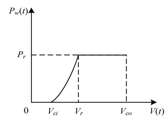
Figure 2.
Variation curve of wind farm output power with wind speed [36].
The following equation can be used to calculate the power output of a wind turbine [33]:
where denotes the wind turbine’s rated power output and , , and denote the cut-in wind speed, rated wind speed, and cut-out wind speed, respectively.
Solar Power Generation
Equation (21) can be used to describe the uncertainty of solar radiation [33]:
where denotes the gamma function, and are the shape parameters of the beta distribution, and and r are the maximal and actual solar radiation value, respectively.
The formulas for and are introduced in [33]. According to the amount of solar radiation r at the installation site, the area of a single solar panel is A, and is the rated conversion efficiency of the PV module, while the output power P of the single PV module with a base power 100 MVA can be calculated as:
2.2.2. Time-Varying Load Forecasting
Since the load demand is not constant, it is necessary to forecast the load demand based on the historical data to evaluate the reliability of the system at a specified time. The term BP neural network refers to the error back propagation (BP) network, which is a multi-layer feedback neural network, first proposed by Rumelhart and McClelland in 1985 [37]. Because of its simple calculation and strong nonlinear mapping, the BP network has been widely used in load prediction and it has been proven to be effective [34]. Thus, this paper adopts this method to forecast three time-varying energy loads. The input layer, hidden layer, and output layer make up the three layers of a BP neural network [34].
An MES power, heat, and gas load forecasting method based on a BP neural network comprises the following steps:
- Input and output vectors are determined according to the specified heat and gas load.
- Construct a BP neural network model according to the input and output vectors.
- Commence network training for the BP neural network.
- Input test samples to conduct a network test on the trained BP neural network, and judge whether the error between the predicted value and the actual value is less than the set threshold. If so, perform Step 5.
- Obtain the required load prediction according to the predicted values.
2.3. Time-Varying Load and Cost Model
The average load is basically a rough estimate of the true load. The time-varying load can be modeled in Equation (23), which includes hourly loads, and provides a more accurate description [29]:
where denotes the annual peak load, is the weekly load as a percentage of the annual peak, is the daily load as a percentage of the weekly peak, and is the hourly load as a percentage of the daily peak.
Because outage loss costs are not constant, a time-varying cost model is required to calculate interruption costs. Customer interruption costs are the financial charges incurred by an electricity consumer as a result of power supply interruptions to their daily activities [38]. In real situations, customer interruption costs for a particular load level and outage period vary depending on the time of occurrence. When an outage happens during peak shopping hours, for example, the cost of interruption to commercial customers is higher than when the outage occurs during off-peak hours. Therefore, by integrating the customer damage function (CDF) with the time-varying cost weight components, a time-varying cost model (TVCM) is constructed for each customer. Since the energy system contains more than one load type, the TVCM for seven typical customer sectors is used to incorporate the time-varying characteristic in the MES reliability evaluation [29].
The following equation calculates the time-varying cost weight factors :
Equation (25) calculates the time-varying cost at hour t by multiplying the appropriate weighting factor with the average interruption cost (AIC) [29]:
3. Reliability Optimization Problem Formulation
To find the optimal location of the storage device in the MES at the lowest possible cost to realize the highest reliability under weather uncertainty, the reliability optimization problem is formulated as a multi-objective problem. The two objective functions to be minimized are based on two performance indicators, i.e., a reliability indicator and an economic indicator. The reliability index, SAIDI, is employed as the reliability indicator to reflect the whole MES reliability performance in this optimization problem. The economic indicator includes both system interruption costs and investment costs. The location of the energy storage device is the decision variable.
3.1. Reliability Indicator
The reliability index, SAIDI, is chosen as the reliability indicator. The formula can be expressed as in Equation (26) [39]:
where is the average outage time of load point i, is the number of customers at load point i, n is the total number of buses, and SY represents the total simulation years.
The average outage time can be calculated as:
where is the number of outage events affecting load point i, is the failure time of load point i, ts and te are the failure start and end points, respectively, and t represents the time step. Whether the load point installs the energy storage device would directly affect its outage time. If the decision variable (the location of the storage device) is not zero, this means that there is a storage device installed. When the failure event happens, if the failure load can be supplied through an energy storage device according to the time series load prediction curves, the number of failures will not be accumulated and the downtime of the system is just the trip time of the automatic switch. Therefore, the relationship between the decision variables and the objective function SAIDI is thus established.
3.2. Economic Indicator
The cost functions, which include the system interruption cost and investment cost, are the economic indicator of the multi-objective functions. The interruption cost is caused by EENS due to the failure of some of the MES components:
where is the outage cost during failure time t at load i, and is expected energy not supplied during failure time t at load i.
The and EENS can be represented as [29]:
where is the average load during failure event j at load point i, is the load demand in the load profile, ts and te are the failure start and end points, respectively, and t represents the time step. Additionally, is defined as the failure duration, and represent time to switch and time to failure affected by failure event j, respectively, and is the load point customer damage function, while is the cost weight factor for hour t.
The investment cost is only the storage device cost because they are the only ones we place and we use them to improve and optimize the system’s reliability:
where N is the total number of the storage devices installed and is the installation cost co-efficient for the storage device i.
3.3. Objective Functions
The optimization problem is formulated as a non-linear problem to find the optimal energy storage configuration schemes. The location of the energy storage device is the decision variable. The two objective functions are formulated as below:
- Objective 1: Minimize the reliability index, SAIDI.
The objective function 1 can be expressed as follows:
- 2.
- Objective 2: Minimize the interruption cost and storage device investment cost.
The objective function 2 can be expressed as follows:
3.4. Constraints
3.4.1. Energy Balance Constraints
The total generations should equal the load demand at each operation time t. The energy balance constraints for the power grid, heat network, and gas network are described in Equations (36)–(38), respectively:
where the left side of the above equation represents total energy generation, while the right side represents the total demands from loads in different energy systems. In addition, t represents the time step, which is one hour.
3.4.2. Energy Storage Devices Constraints
The charging and discharging power of ES (Equations (39) and (40)), HS (Equations (41) and (42)), and GS (Equation (43)) are bounded by their minimum and maximum values. Moreover, the total flow in and flow out power should be balanced at all time steps (Equations (44) and (45)). The capacity of ES, HS, and GS cannot exceed the maximum limit, according to Equations (46)–(48), respectively:
where represents the electricity of ES at hour t and is the capacity of ES.
3.4.3. PV and Wind Turbine Constraints
The capacity constraints for PV and wind turbines are expressed in Equations (49) and (50):
3.5. Normalization of Objective Functions
Due to the magnitudes of the two objective functions differing, normalizing the objectives is necessary to obtain a Pareto optimal solution.
First, we optimize each of the objective functions (Equations (34) and (35)) individually using the single objective function to obtain the maximum and minimum values of each objective function. Assume i is the sequence number of the objective function, then, after normalization, all objective functions will be constrained by [40]:
because we normalize the objective functions by the real intervals of their variation throughout the Pareto optimum set, and this gives all the objective functions the same magnitude (0–1) [41].
3.6. Problem Formulation
The multi-objective reliability optimization problem is therefore formulated as:
subject to Equations (36)–(50).
3.7. Multi-Objective Optimization Algorithms
The NSGA-II, SPEA2, and MOPSO algorithms are multi-objective stochastic optimization algorithms. NSGA-II is an improved version of the non-dominated sorting genetic algorithm (NSGA) [26]. NSGA-II emphasizes the non-dominated sorting with the elitist principle by passing the best non-dominated solutions to the next generation. It also uses a crowded distance-based diversity-preserving mechanism to find the nearest solution belonging to the Pareto front to be reserved for the next generation [42]. SPEA2 is a multi-objective optimization algorithm [43] that has four main features: (a) the external archive stores the non-dominated solution in a continuously updating population, (b) the number of external non-dominated points that dominate an individual’s fitness is used to assess their fitness, (c) the Pareto dominance relationship is used to maintain population diversity, and (d) the clustering process is introduced to decrease the non-dominated set without destroying the properties of the non-dominated set. MOPSO [28] determines a particle’s flight direction using the Pareto dominance principle, and it stores previously discovered non-dominated vectors in a global repository that is then used by other particles to guide their flight. All the algorithms above are based on a non-dominated sorting mechanism. By comparing the values of the same objective, non-dominated sorting divides a solution set into numerous disjointed subsets or ranks. Solutions of the same rank are considered to be equally important after non-dominated sorting, and solutions of lower ranks are preferred over those of higher ranks [44]. The adaptive stop criterion (also known as the stagnation criterion) is used as the stop criterion, whereby the algorithm stops when the objective function converges to the optimal value and does not change after a certain number of iterations. Moreover, setting the maximum number of iterations to an exceptionally high value might be used as a last-resort resource stop criterion to catch infinite executions [21].
The optimization process related to all three algorithms is shown in Figure 3, and the optimization steps are as follows:
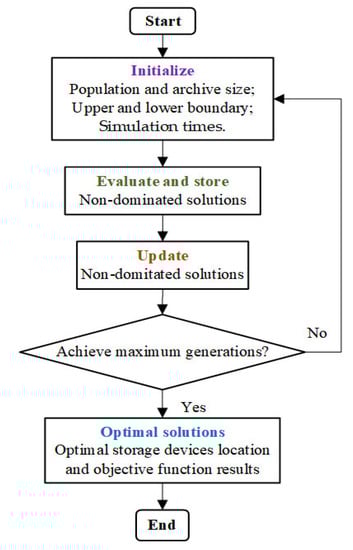
Figure 3.
The reliability optimization flow chart.
- Step 1:
- Initialize population, generation size, the upper and lower boundary of decision variables (the placement of each particle should not exceed its energy network total buses), and simulation times.
- Step 2:
- Evaluate the objective functions using Monte Carlo simulation and store the non-dominated solutions in the repository.
- Step 3:
- Update the non-dominated solution.
- Step 4:
- Stop if the adaptive stop criterion and the maximum number of generations have been achieved; otherwise, proceed to step 2.
- Step 5:
- Obtain optimal solutions: optimal storage devices placement schemes and objective functions results.
4. Case Study
A case study is developed to demonstrate the applicability of the proposed technique. A comparative analysis is conducted where widely used multi-objective algorithms, i.e., NSGA-II, MOPSO, and SPEA2, are applied to solve the formulated reliability optimization problem illustrated in Section 3. The considered MES includes an IEEE 39 bus system [45], a 32-node heat network [46], and a 20-node Belgian natural gas network [47]. Figure 4 depicts a schematic diagram of the tested multi-energy system. Besides generators in the power grid, the PV, WT, GT, and V2G systems have been considered in the MES design for providing supplemental energy to the critical load demands, which have been installed on buses 1, 2, 20, and 26 respectively. The coupling components, such as CHP, P2G, and V2G, can enable multi-energy flows and improve energy efficiency in the MES.
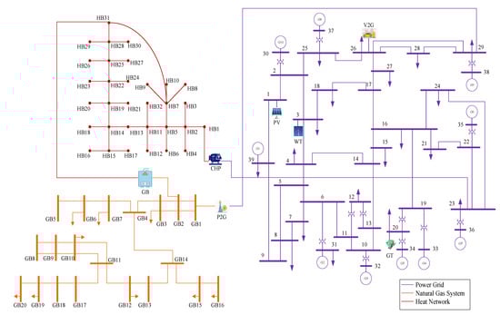
Figure 4.
The schematic diagram of the multi-energy system.
4.1. Simulation Parameters
The reliability evaluation and optimization of the MES are developed with MATLAB 2020b on a PC with an Intel® Core™ i5-7200 2.5 GHz CPU and 8 GB RAM. The simulation period for the MCS reliability evaluation is set as 20 years with a time step of one hour, with 100 MCS runs at each iteration to obtain reasonable results. The parameters for the Weibull distribution and beta distribution in the uncertainty modeling of a wind farm and PV are shown in Table 1 and Table 2, respectively [33].

Table 1.
Weibull distribution parameters.
Table 2.
Beta distribution parameters.
The probability distributions for wind speed and solar radiation are shown in Figure 5.
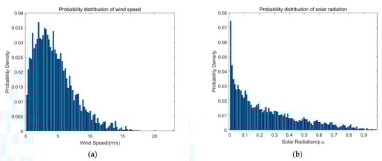
Figure 5.
(a) Weibull distribution of wind speed; (b) beta distribution of solar radiation.
The parameters for forecasting power, heat, and natural gas loads are presented in the following Table 3 [35]. The BP neural network is used to forecast future load changes based on historical data.
Table 3.
BP neural network parameters.
The load forecast result for the MES is shown in the following Figure 6. The training results show that the relative error of all loads is less than 0.2, which has met the training goal. The maximum absolute error is 0.01 in the IEEE 39 power system, 0.004 in the 32-node heat network, and 0.13 in the 20-node Belgian natural gas network.
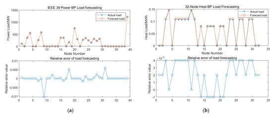
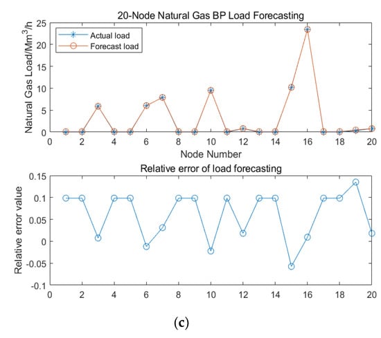
Figure 6.
BP neural network load forecasting for: (a) IEEE 39 bus system; (b) 32-node heat network; (c) 20-node natural gas network.
The sequential Monte Carlo simulation method is used to assess the multi-energy system’s reliability. The failure rate and repair time of the components in the MES can be found in [9]. The installation cost and capacity for different types of storage devices are given in Table 4. The capacities of PV, WT, and GT are shown in Table 5. The interruption cost for seven types of customers and failure duration can be found in [29]. The seven typical customer types are composited by large user, industry, commerce, agriculture, resident, government, and office. The time-varying cost weight factor profiles in terms of seven customers over 24 h are presented in [29]. The load and customer data of the IEEE 39 bus system, 32-node heat network, and 20-node Belgian natural gas network can be found in Appendix Table A1, Table A2 and Table A3, respectively [45,46,47].
Table 4.
The installation cost coefficient and capacity for storage devices.
Table 5.
The capacity of PV, WT, and GT.
NSGA-II, MOPSO, and SPEA2 algorithms have been used to obtain the optimal case for different storage devices. In order to select the reasonable parameters, the parameters have been tested through experiments. The population size, number of generations, and mutation rate start from low values, while the crossover rate starts from a high value, given that it will begin decreasing. The population size and number of generations can have an impact on the execution time. For MOPSO, a large population size is needed as it requires a longer execution time compared to the other two algorithms. The NSGA-II, MOPSO, and SPEA2 parameters are summarized in Table 6 [48]. Before running the optimization, it is vital to determine the population size, maximum generations, and their repository/archive size. For MOPSO, the accelerating parameters and are used to update the velocity and position of each particle, whereas for NSGA-II and SPEA2, crossover and mutation factors are required to conduct non-dominated sorting to obtain the offspring generation and subsequently find out the global optimal solution.
Table 6.
Multi-objective optimization algorithm parameters.
4.2. Simulation Results
Figure 7 gives the convergence characteristics of the two objectives. All the three algorithms converge to their minimum values and the adaptive stop criterion has been satisfied before the maximum number of iterations is reached, and no early stopping (the optimization stops early even though the objective function continues to provide considerable improvements) or late stopping (the optimization stops with no significant improvement for many of the last generations) [21] occurs. The convergence characteristics of the NSGA-II, MOPSO, and SPEA2 are thus proved.
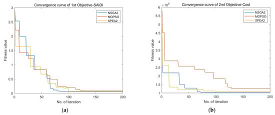
Figure 7.
Convergence curve of: (a) SAIDI; (b) cost.
Figure 8 gives the Pareto front results of the three algorithms. Among them, NSGA-II converges the fastest, followed by SPEA2. The Pareto front shown in Figure 8 has been devised by applying the three multi-objective optimization algorithms described in Section 3 to solve the reliability optimization problems listed in Equations (34) and (35). The horizontal and vertical coordinates represent the two objective functions. It can be noted that the NSGA-II method leads to better optimal values of the objective functions compared to the other two methods, resulting in a high-quality solution.
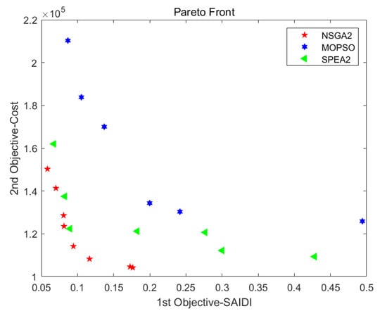
Figure 8.
Pareto front results of three multi-objective algorithms.
The optimal results obtained from the three different algorithms are summarized in Table 7, Table 8 and Table 9 All three tables are sorted in order of cost from high to low. Since higher reliability costs more money and the cost function relates to the interruption cost and storage device investment cost, users can decide their optimal case based on the given tables. NSGA-II costs only USD 1.5028 × 105 × 1000 and achieves a SAIDI value of 0.0585, given in the number one case for NSGA-II, whereas MOPSO costs USD 2.1029 × 105 × 1000 and achieves the lowest SAIDI value of 0.0867, and SPEA2 costs USD 1.6200 × 105 × 1000 and achieves the lowest SAIDI value of 0.0673. From the three tables, it is not difficult to find out that SPEA2 outperformed MOPSO, but underperformed NSGA-II. However, it should be pointed out that higher reliability does not mean more storage devices, for MES reliability would relate to both storage device placement and the system interruption costs, and the second set of data has 41 storage devices while the fourth set of data has 49 storage devices in NSGA-II results, which can reflect this point of view. Table 10 compares the computational times of these three algorithms. It can be seen that NSGA-II and SPEA2 are faster than MOPSO.
Table 7.
NSGA-II optimization result.
Table 8.
MOPSO optimization result.
Table 9.
SPEA2 optimization result.
Table 10.
Comparison of execution times.
Table 11 compares the reliability indices of the MES before and after optimization. As energy storage devices are added, there are more components, resulting in a modest rise in the SAIFI (system average interruption frequency index) value. The system average interruption duration (SAIDI) decreased by 96.12%, from 1.4945 h/Ca to 0.0585 h/Ca. The customer average interruption duration (CAIDI) decreased by 99.21%, from 7.548 h/Ca to 0.0600 h/Ca. As for the average service availability, ASAI reached a high level, and the optimization to ASAI is very small. Even though the ASAI rise was minor, the system outage time was significantly reduced.
Table 11.
Comparison of reliability indices before and after optimization.
In fact, there are numerous scholars who have conducted a comparison study between the NSGA-II, SPEA2, and MOPSO algorithms, which would help to understand the optimization results. The authors in [49] have tested several MOEAs on ZDT and WFG functions, and the results reveal that no algorithm can always be superior or worse than other algorithms on all test functions. A portfolio optimization problem has been studied in [50] to compare the performance of NSGA-II, SPEA2, and MOPSO, and the results suggests that MOPSO outperforms the other two. However, in the stochastic optimization problem of an inventory control system in [51], NSGA-II outperforms MOPSO in terms of spacing and the number of Pareto optimal solutions. Therefore, in view of the reliability optimization problem raised in this paper, the case study results indicate that the NSGA-II algorithm leads to better optimal values and converges the fastest compared to the other two methods. The results can be varied depending on different test problems.
5. Conclusions and Future Work
This paper proposes a methodology for reliability optimization in a multi-energy system with storage devices considering the weather uncertainties using NSGA-II, MOPSO, and SPEA2. Moreover, the multi-objective reliability optimization problem is formulated as a non-linear problem to find the optimal energy storage configuration schemes, which can improve MES reliability. The feasibility of the proposed method has been proven on a typical MES, which includes an IEEE 39 bus system, a 32-node heat network, and a 20-node Belgian natural gas network. From the simulation results, we find that NSGA-II outperforms two other modern optimization algorithms, MOPSO and SPEA2, as it can maintain a wider range of solutions and converge faster in the non-dominated front. NSGA-II can converge closer to the true Pareto optimal front, has the fastest computational time, and is found to be the best among the three approaches studied here. Higher reliability may result in a more expensive cost in terms of the storage device cost, but reduce system interruption time, and the customer can choose the optimal case based on their situation.
As for future work, more studies could be performed on risk analysis or vulnerability modeling of the multi-energy system. The robust and resilient operation and control of the multi-energy system can also be considered as the future scope of this research.
Author Contributions
Z.L.: Conceptualization, Methodology, Software, Validation, Formal analysis, Investigation, Resources, Data curation, Visualization, Writing—original draft preparation; A.P.: Supervision, Project administration, Writing—review and editing. All authors have read and agreed to the published version of the manuscript.
Funding
This research received no external funding.
Institutional Review Board Statement
Not applicable.
Informed Consent Statement
Not applicable.
Data Availability Statement
Not applicable.
Conflicts of Interest
The authors declare no conflict of interest.
Abbreviations
| MES | Multi-energy system |
| MCS | Monte Carlo simulation |
| NSGA-II | Non-dominated sorting genetic algorithm II |
| MOPSO | Multiple objective particle swarm optimization |
| SPEA2 | Strength Pareto evolution algorithm 2 |
| MOEA | Multi-objective evolutionary algorithm |
| CHP | Combined heat and power |
| P2G | Power to gas |
| GB | Gas boiler |
| PG | Power grid |
| HN | Heat network |
| GN | Gas network |
| CCHP | Combined cooling, heat, and power |
| V2G | Vehicle to grid |
| FMEA | Failure mode and effect analysis |
| ES | Electricity storage |
| HS | Heat storage |
| GS | Gas storage |
| TVCM | Time-varying cost model |
| CDF | Customer damage function |
| SAIFI | System average interruption frequency index |
| SAIDI | System average interruption duration index |
| CAIDI | Customer average interruption duration index |
| ASAI | Average service availability index |
| EENS | Expected energy not supplied |
| TTF | Time to failure |
| TTR | Time to repair |
| TTS | Time to switch |
Appendix A
There are seven customer types, which are represented by “1-Industrial”, “2-Agriculture”, “3-Large user”, “4-Commercial”, “5-Government”, “6-Office”, and “7-Residential”.
Table A1.
An IEEE 39 bus system load and customer data [45].
Table A1.
An IEEE 39 bus system load and customer data [45].
| Load Points | Average Load Level (MW) | Customer Type | Number of Customers |
|---|---|---|---|
| 1 | 97.6 | 7 | 200 |
| 3 | 322 | 7 | 322 |
| 4 | 500 | 4 | 500 |
| 7 | 233.8 | 5 | 200 |
| 8 | 522 | 6 | 500 |
| 9 | 6.5 | 7 | 132 |
| 12 | 8.53 | 3 | 23 |
| 15 | 320 | 4 | 320 |
| 16 | 329 | 6 | 330 |
| 18 | 158 | 3 | 160 |
| 20 | 680 | 2 | 680 |
| 21 | 274 | 6 | 270 |
| 23 | 247.5 | 7 | 240 |
| 24 | 308.6 | 7 | 300 |
| 25 | 224 | 7 | 220 |
| 26 | 139 | 7 | 140 |
| 27 | 281 | 7 | 280 |
| 28 | 206 | 7 | 200 |
| 29 | 283.5 | 7 | 280 |
| 31 | 9.2 | 1 | 60 |
| 39 | 522 | 6 | 1000 |
Table A2.
A 32-node heat network load and customer data [46].
Table A2.
A 32-node heat network load and customer data [46].
| Load Points | Average Load Level (MW) | Customer Type | Number of Customers |
|---|---|---|---|
| 3 | 0.107 | 1 | 110 |
| 4 | 0.145 | 3 | 150 |
| 6 | 0.107 | 4 | 110 |
| 7 | 0.107 | 5 | 110 |
| 8 | 0.107 | 6 | 110 |
| 9 | 0.107 | 3 | 110 |
| 10 | 0.107 | 1 | 110 |
| 11 | 0.145 | 6 | 150 |
| 12 | 0.107 | 7 | 110 |
| 14 | 0.0805 | 7 | 80 |
| 16 | 0.0805 | 7 | 80 |
| 17 | 0.0805 | 7 | 80 |
| 18 | 0.0805 | 7 | 80 |
| 20 | 0.0805 | 7 | 80 |
| 21 | 0.0805 | 7 | 80 |
| 23 | 0.107 | 2 | 110 |
| 24 | 0.107 | 4 | 110 |
| 26 | 0.107 | 6 | 110 |
| 27 | 0.107 | 7 | 110 |
| 29 | 0.107 | 3 | 110 |
| 30 | 0.107 | 7 | 110 |
Table A3.
A 20-node Belgian natural gas system load and customer data [47].
Table A3.
A 20-node Belgian natural gas system load and customer data [47].
| Load Points | Average Load Level (Mm3/day) | Customer Type | Number of Customers |
|---|---|---|---|
| 3 | 5.88 | 1 | 60 |
| 6 | 6.05 | 5 | 61 |
| 7 | 7.88 | 3 | 80 |
| 10 | 9.55 | 4 | 100 |
| 12 | 0.775 | 7 | 80 |
| 15 | 10.27 | 2 | 105 |
| 16 | 23.42 | 6 | 240 |
| 19 | 0.33 | 7 | 30 |
| 20 | 0.775 | 7 | 80 |
References
- Kueck, J.D. Measurement Practices for Reliability and Power Quality; Oak Ridge Nat. Lab. (ORNL): Oak Ridge, TN, USA, 2005.
- Zhang, S.; Wen, M.; Cheng, H.; Hu, X.; Xu, G. Reliability evaluation of electricity-heat integrated energy system with heat pump. CSEE J. Power Energy Syst. 2018, 4, 425–433. [Google Scholar] [CrossRef]
- Billinton, R.; Jonnavithula, S. A test system for teaching overall power system reliability assessment. IEEE Trans. Power Syst. 1996, 11, 1670–1676. [Google Scholar] [CrossRef] [Green Version]
- He, J.; Yuan, Z.; Yang, X.; Huang, W.; Tu, Y.; Li, Y. Reliability modeling and evaluation of urban multi-energy systems: A review of the state of the art and future challenges. IEEE Access 2020, 8, 98887–98909. [Google Scholar] [CrossRef]
- Wang, J.; Fu, C.; Yang, K. Reliability and availability analysis of redundant BCHP (building cooling, heating and power) system. Energy 2013, 61, 531–540. [Google Scholar] [CrossRef]
- Munoz, J.; Jimenez-Redondo, N.; Perez-Ruiz, J.; Barquin, J. Natural gas network modeling for power systems reliability studies. In Proceedings of the IEEE Bologna Power Tech Conference, Bologna, Italy, 23–26 June 2003; Volume 4, p. 8. [Google Scholar]
- Chaudry, M.; Wu, J.; Jenkins, N. A sequential Monte Carlo model of the combined GB gas and electricity network. Energy Policy 2013, 62, 473–483. [Google Scholar] [CrossRef]
- Gargari, Z.; Ghaffarpour, R. Reliability evaluation of multi-carrier energy system with different level of demands under various weather situation. Energy 2020, 196, 117091. [Google Scholar] [CrossRef]
- Meng, Z.; Wang, S.; Zhao, Q.; Zheng, Z.; Feng, L. Reliability evaluation of electricity-gas-heat multi-energy consumption based on user experience. Int. J. Electr. Power Energy Syst. 2021, 130, 106926. [Google Scholar] [CrossRef]
- Koeppel, G.; Andersson, G. Reliability modeling of multi-carrier energy systems. Energy 2009, 34, 235–244. [Google Scholar] [CrossRef]
- Ge, S.; Li, J.; Liu, H.; Wang, Y.; Sun, H.; Lu, Z. Reliability evaluation of microgrid containing energy storage system considering multi-energy coupling and grade difference. Autom. Electr. Power Syst. 2018, 42, 165–173. [Google Scholar]
- Ge, S.; Sun, H.; Liu, H.; Li, J.; Zhang, X.; Cao, Y. Reliability evaluation of multi-energy microgrids: Energy storage devices effects analysis. Energy Procedia 2019, 158, 4453–4458. [Google Scholar] [CrossRef]
- Ammous, M.; Khater, M.; AlMuhaini, M. Impact of vehicle-to-grid technology on the reliability of distribution systems. In Proceedings of the 9th IEEE-GCC Conference and Exhibition, Manama, Bahrain, 8–11 May 2017; pp. 1–6. [Google Scholar]
- Bakkiyaraj, R.A.; Kumarappan, N. Optimal reliability planning for a composite electric power system based on Monte Carlo simulation using particle swarm optimization. Int. J. Electr. Power Energy Syst. 2013, 47, 109–116. [Google Scholar] [CrossRef]
- Barakat, S.; Ibrahim, H.; Elbaset, A.A. Multi-objective optimization of grid-connected PV-wind hybrid system considering reliability, cost, and environmental aspects. Sustain. Cities Soc. 2020, 60, 102178. [Google Scholar] [CrossRef]
- Peruzzi, L.; Salata, F.; de Lieto Vollaro, A.; de Lieto Vollaro, R. The reliability of technological systems with high energy efficiency in residential buildings. Energy Build. 2014, 68, 19–24. [Google Scholar] [CrossRef]
- Kanase-Patil, A.B.; Saini, R.P.; Sharma, M.P. Sizing of integrated renewable energy system based on load profiles and reliability index for the state of Uttarakhand in India. Renew. Energy 2011, 36, 2809–2821. [Google Scholar] [CrossRef]
- Arnold, M. On Predictive Control for Coordination in Multi-Carrier Energy Systems. Ph.D. Thesis, ETH Zurich, Zurich, Switzerland, 2011. [Google Scholar]
- Raychaudhuri, S. Introduction to Monte Carlo simulation. In Proceedings of the Winter Simulation Conference, Miami, FL, USA, 7–10 December 2008; pp. 91–100. [Google Scholar]
- Billinton, R.; Li, W. A system state transition sampling method for composite system reliability evaluation. IEEE Trans. Power Syst. 1993, 8, 761–770. [Google Scholar] [CrossRef]
- Chicco, G.; Mazza, A. Metaheuristic optimization of power and energy systems: Underlying principles and main issues of the rush to heuristic. Energies 2020, 13, 5097. [Google Scholar] [CrossRef]
- Lee, K.Y.; El-Sharkawi, M.A. Modern Heuristic Optimization Techniques: Theory and Applications to Power Systems; John Wiley & Sons: Hoboken, NJ, USA, 2008; Volume 39. [Google Scholar]
- Lee, K.Y.; Vale, Z.A. Applications of Modern Heuristic Optimization Methods in Power and Energy Systems; John Wiley & Sons: Hoboken, NJ, USA, 2020. [Google Scholar]
- Chicco, G.; Mazza, A. Heuristic optimization of electrical energy systems: Refined metrics to compare the solutions. Sustain. Energy Grids Netw. 2019, 17, 100197. [Google Scholar] [CrossRef] [Green Version]
- Oteiza, P.P.; Rodríguez, D.A.; Brignole, N.B. Parallel cooperative optimization through hyperheuristics. Comput. Aided Chem. Eng. 2018, 44, 805–810. [Google Scholar]
- Deb, K.; Agrawal, S.; Pratap, A.; Meyarivan, T. A fast elitist non-dominated sorting genetic algorithm for multi-objective optimization: NSGA-II. In Proceedings of the International Conference on Parallel Problem Solving from Nature, Leiden, The Netherlands, 5–9 September 2000; pp. 849–858. [Google Scholar]
- Kunkle, D. A Summary and Comparison of Moea Algorithms. Internal Report. 2005. Available online: https://www.ccs.neu.edu/home/kunkle/papers/techreports/moeaComparison.pdf (accessed on 5 January 2022).
- Coello, C.A.C.; Pulido, G.T.; Lechuga, M.S. Handling multiple objectives with particle swarm optimization. IEEE Trans. Evol. Comput. 2004, 8, 256–279. [Google Scholar] [CrossRef]
- Wang, P.; Billinton, R. Time sequential distribution system reliability worth analysis considering time varying load and cost models. IEEE Trans. Evol. Comput. 2004, 8, 256–279. [Google Scholar]
- Li, Y.; Zhang, F.; Li, Y.; Wang, Y. An improved two-stage robust optimization model for CCHP-P2G microgrid system considering multi-energy operation under wind power outputs uncertainties. Energy 2021, 223, 120048. [Google Scholar] [CrossRef]
- Shi, N.; Luo, Y. Energy storage system sizing based on a reliability assessment of power systems integrated with wind power. Sustainability 2017, 9, 395. [Google Scholar] [CrossRef] [Green Version]
- Ogunmodede, O.; Anderson, K.; Cutler, D.; Newman, A. Optimizing design and dispatch of a renewable energy system. Appl. Energy 2021, 287, 116527. [Google Scholar] [CrossRef]
- Prajapati, V.K.; Mahajan, V. Reliability assessment and congestion management of power system with energy storage system and uncertain renewable resources. Energy 2021, 215, 119134. [Google Scholar] [CrossRef]
- Wu, G.; Zu, G.; Zheng, J. A method for forecasting alpine area load based on artificial neural network model. J. Phys. Conf. Ser. 2021, 1994, 12019. [Google Scholar] [CrossRef]
- Borges, C.E.; Penya, Y.K.; Fernandez, I. Evaluating combined load forecasting in large power systems and smart grids. IEEE Trans. Ind. Info. 2013, 9, 1570–1577. [Google Scholar] [CrossRef]
- Monnerie, N.; Houaijia, A.; Roeb, M.; Sattler, C. Methane production via high temperature steam electrolyser from renewable wind energy: A german study. Green Sustain. Chem. 2015, 5, 70–80. [Google Scholar] [CrossRef] [Green Version]
- Niu, D.; Shi, H.; Li, J.; Wei, Y. Research on short-term power load time series forecasting model based on BP neural network. In Proceedings of the 2nd International Conference on Advanced Computer Control, Shenyang, China, 27–29 March 2010; Volume 4, pp. 509–512. [Google Scholar]
- Dzobo, O.; Awodele, K.O. Probabilistic Power System Reliability Assessment: Distributed Renewable Energy Sources. In Novel Advancements in Electrical Power Planning and Performance; IGI Global: Hershey, PA, USA, 2020; pp. 94–117. [Google Scholar]
- Tur, M.R. Reliability assessment of distribution power system when considering energy storage configuration technique. IEEE Access 2020, 8, 77962–77971. [Google Scholar] [CrossRef]
- Xu, Y.; Zhang, G.; Yan, C.; Wang, G.; Jiang, Y.; Zhao, K. A two-stage multi-objective optimization method for envelope and energy generation systems of primary and secondary school teaching buildings in China. Build. Environ. 2021, 204, 108142. [Google Scholar] [CrossRef]
- Grodzevich, O.; Romanko, O. Normalization and other topics in multi-objective optimization. In Proceedings of the Fields–MITACS Industrial Problems Workshop, Toronto, ON, Canada, 14–18 August 2006; Available online: http://miis.maths.ox.ac.uk/miis/233/1/fmipw1-6.pdf (accessed on 5 January 2022).
- Verma, S.; Pant, M.; Snasel, V. A Comprehensive review on NSGA-II for multi-objective combinatorial optimization problems. IEEE Access 2021, 9, 57757–57791. [Google Scholar] [CrossRef]
- Zitzler, E.; Thiele, L. Multi objective evolutionary algorithms: A comparative case study and the strength Pareto approach. IEEE Trans. Evol. Comput. 1999, 3, 257–271. [Google Scholar] [CrossRef] [Green Version]
- Tian, Y.; Wang, H.; Zhang, X.; Jin, Y. Effectiveness and efficiency of non-dominated sorting for evolutionary multi-and many-objective optimization. Complex Intell. Syst. 2017, 3, 247–263. [Google Scholar] [CrossRef]
- Real Time Power System Simulation I RTDS Technologies. Available online: http://www.rtds.com/indexlindex.Html (accessed on 5 January 2022).
- Liu, X.; Wu, J.; Jenkins, N.; Bagdanavicius, A. Combined analysis of electricity and heat networks. Appl. Energy 2016, 162, 1238–1250. [Google Scholar] [CrossRef] [Green Version]
- Zhang, H.; Zhao, T.; Wang, P.; Yao, S. Power system resilience assessment considering of integrated natural gas system. In Proceedings of the IET International Conference on Resilience of Transmission and Distribution Networks, Birmingham, UK, 26–28 September 2017; pp. 1–7. [Google Scholar]
- Jain, A.; Lalwani, S.; Lalwani, M. A comparative analysis of MOPSO, NSGA-II, SPEA2 and PESA2 for multi-objective optimal power flow. In Proceedings of the 2nd International Conference on Power, Energy and Environment: Towards Smart Technology (ICEPE), Shillong, India, 1–2 June 2018; pp. 1–6. [Google Scholar]
- Yu, X.; Lu, Y.; Yu, X. Evaluating multi-objective evolutionary algorithms using MCDM methods. Math. Probl. Eng. 2018, 2018, 9751783. [Google Scholar] [CrossRef] [Green Version]
- Mishra, S.K.; Panda, G.; Meher, S. Multi-objective particle swarm optimization approach to portfolio optimization. In Proceedings of the World Congress on Nature & Biologically Inspired Computing (NaBIC) Conference, Coimbatore, India, 9–11 December 2009; pp. 1612–1615. [Google Scholar]
- Keshavarz, M.; Pasandideh, S.H.R. Multi-objective optimisation of continuous review inventory system under mixture of lost sales and backorders within different constraints. Int. J. Logist. Syst. Manag. 2018, 29, 327–348. [Google Scholar]
Publisher’s Note: MDPI stays neutral with regard to jurisdictional claims in published maps and institutional affiliations. |
© 2022 by the authors. Licensee MDPI, Basel, Switzerland. This article is an open access article distributed under the terms and conditions of the Creative Commons Attribution (CC BY) license (https://creativecommons.org/licenses/by/4.0/).