
Evaluation Metrics for Wind Power Forecasts: A Comprehensive Review and Statistical Analysis of Errors


Abstract
1. Introduction
1.1. Major Factors Affecting Wind Power Forecasts
1.2. Objective and Contribution
- classify wind power forecasting techniques;
- provide unique description of major factors affecting wind power forecasts;
- describe the performance of forecasting models;
- conduct comprehensive review (quantitative analysis) based on more than one hundred papers;
- conduct statistical analysis of errors (qualitative analysis).
- proposal for a novel, unique ratio, called EDF;
- analysis of variability of the new EDF ratio depending on selected characteristics (size of wind farm, forecasting horizon, and class of forecasting method) and the original, novel conclusions drawn from the analysis;
- development of a unique list of recommended content of papers addressing wind farm generation forecasts (the application of these recommendations would make it possible to conduct very accurate meta-analyses that would compare various forecasting studies).
2. Classification of Wind Power Forecasting Techniques
3. Performance of Forecasting Model
3.1. RMSE, MAE, and MAPE as Frequently-Used Metrics
3.2. MSE, nMAE, nRMSE, and R2 As Occasionally Used Metrics
3.3. R, PICP, PINAW, sMAPE, MRE, and TIC As Seldom Used Metrics
3.4. Interesting Usage of Other Metrics
4. Comprehensive Statistical Analysis
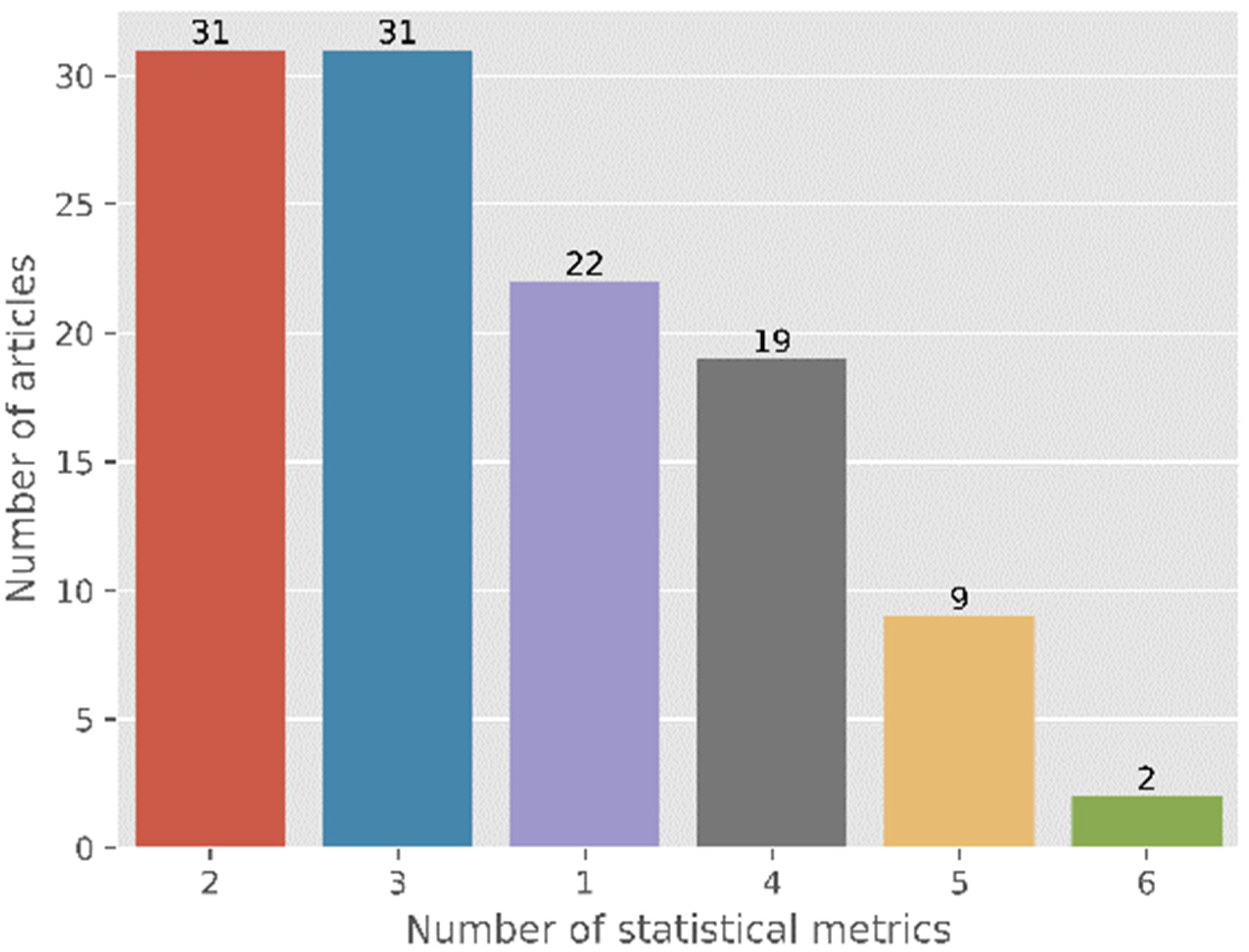
4.1. Comprehensive Quantitative Review
4.2. Comprehensive Error Analysis
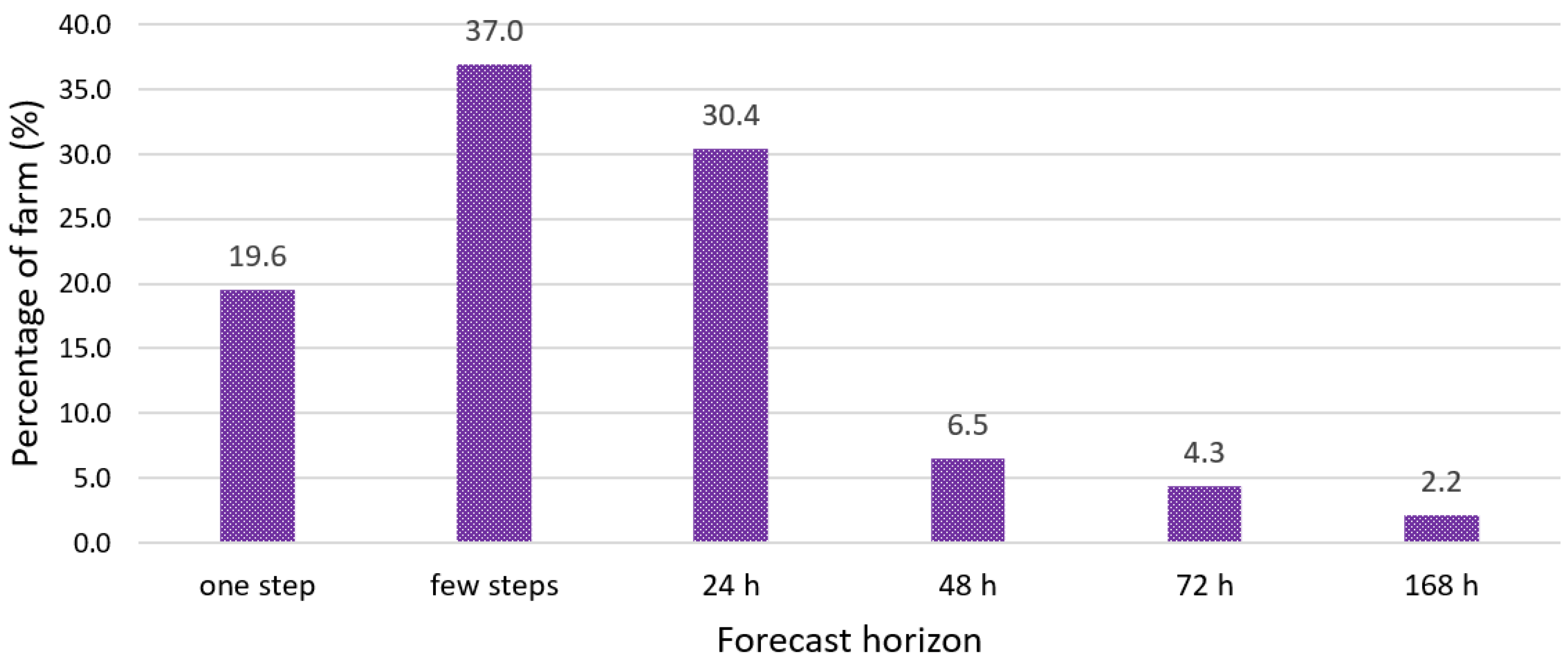
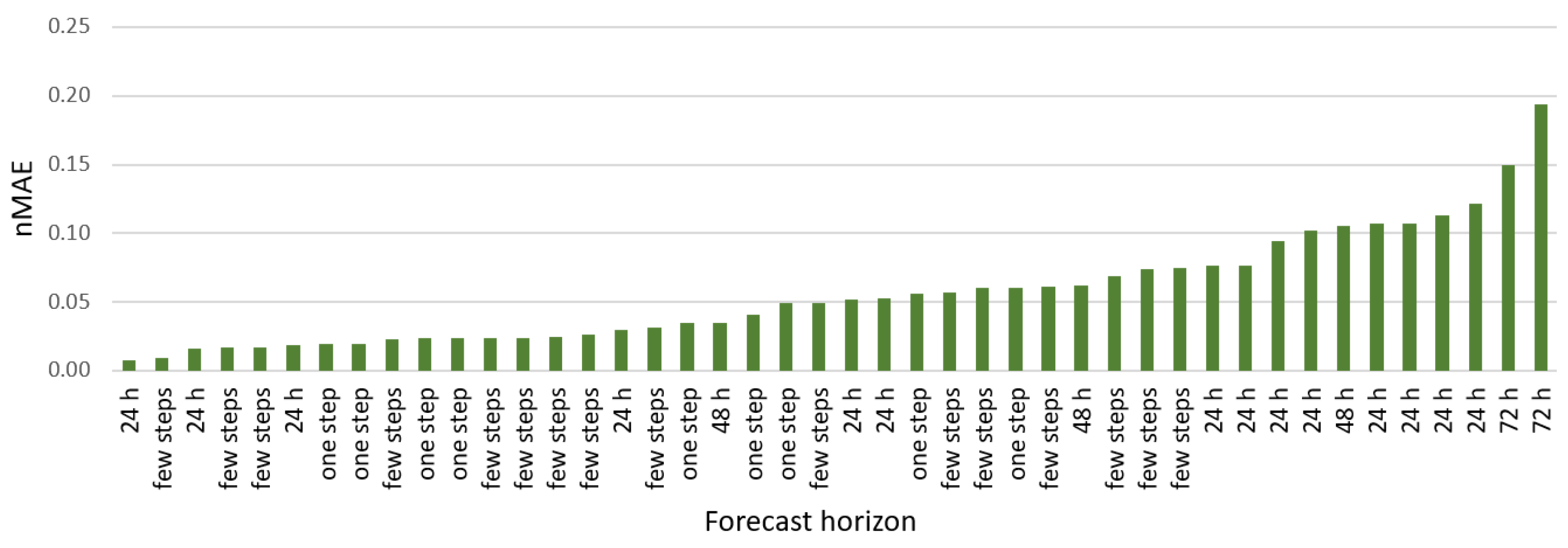
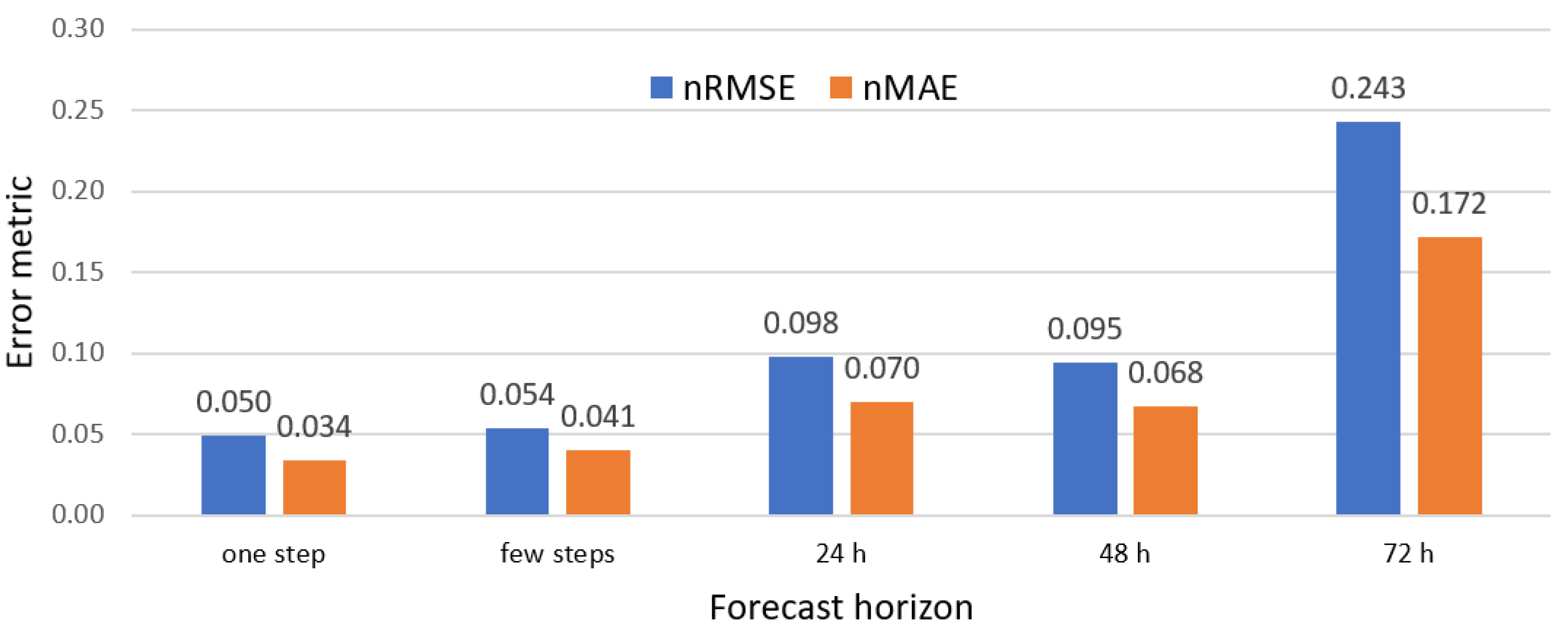
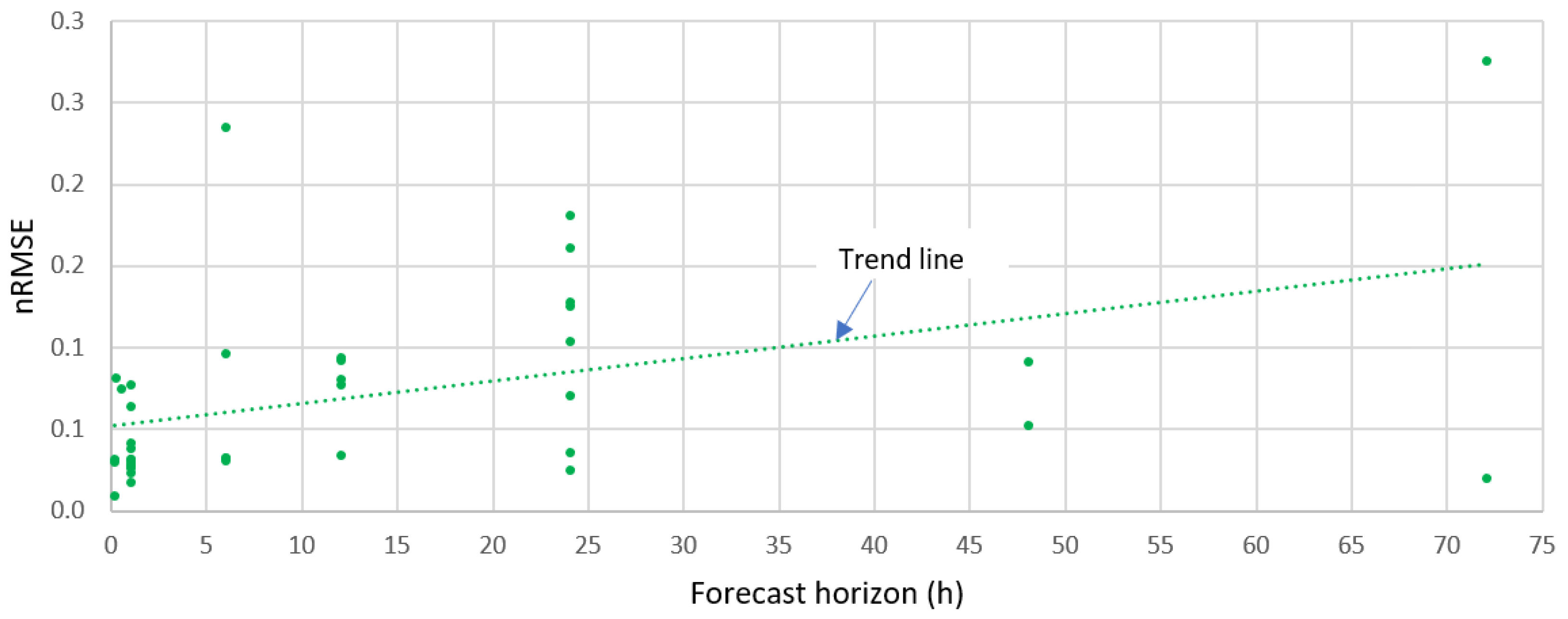
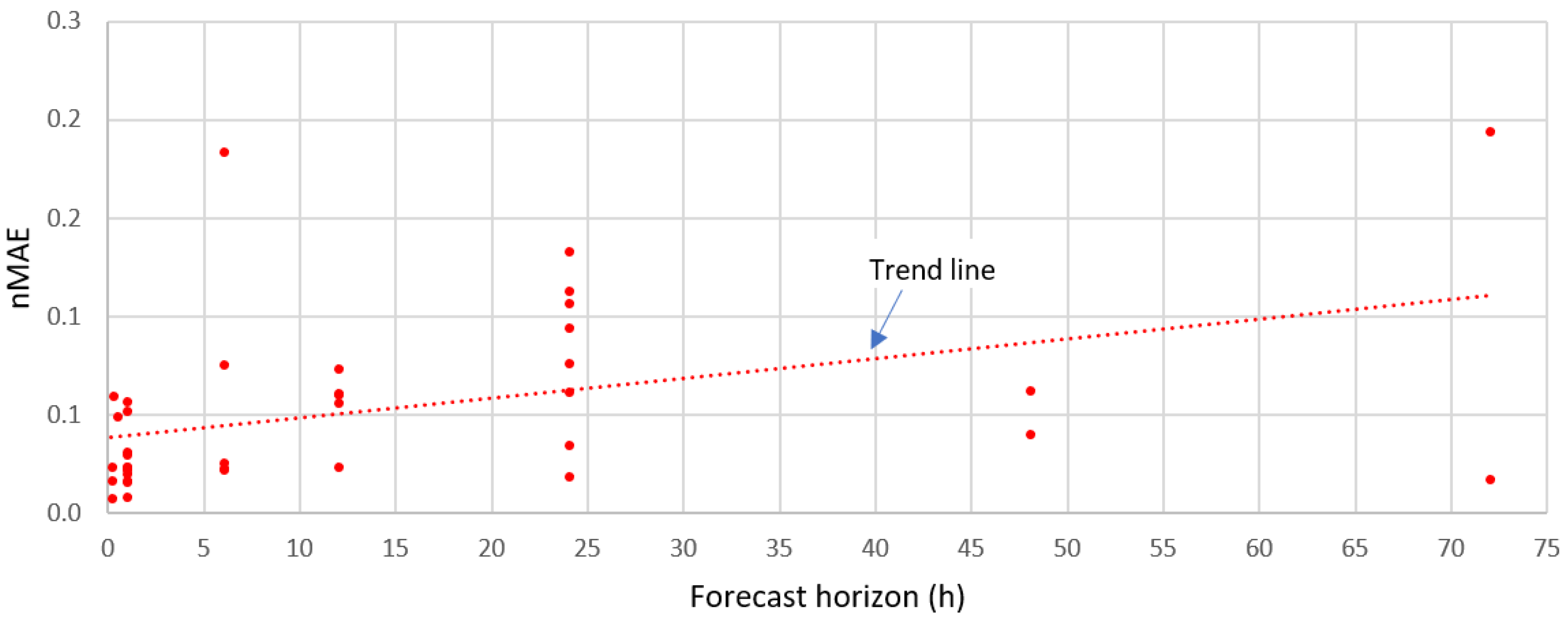
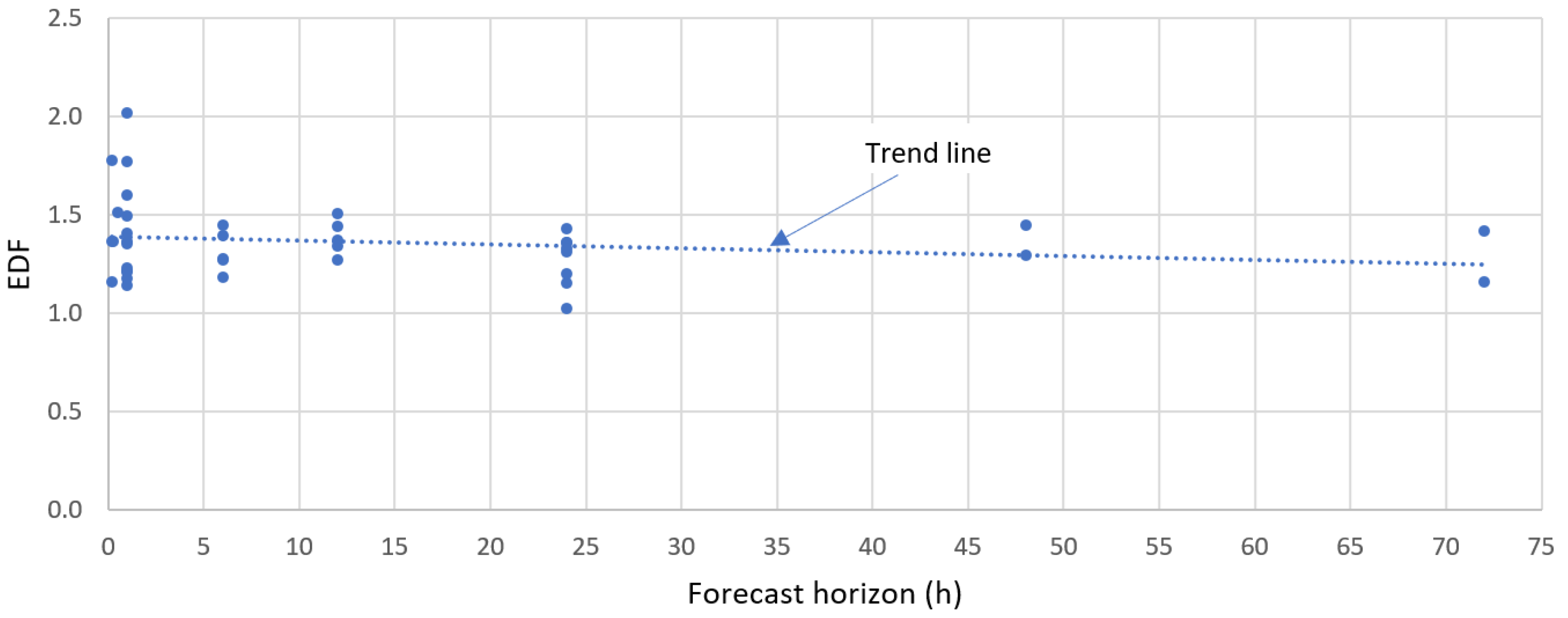
4.2.1. Analysis of Errors by Forecasting Horizon
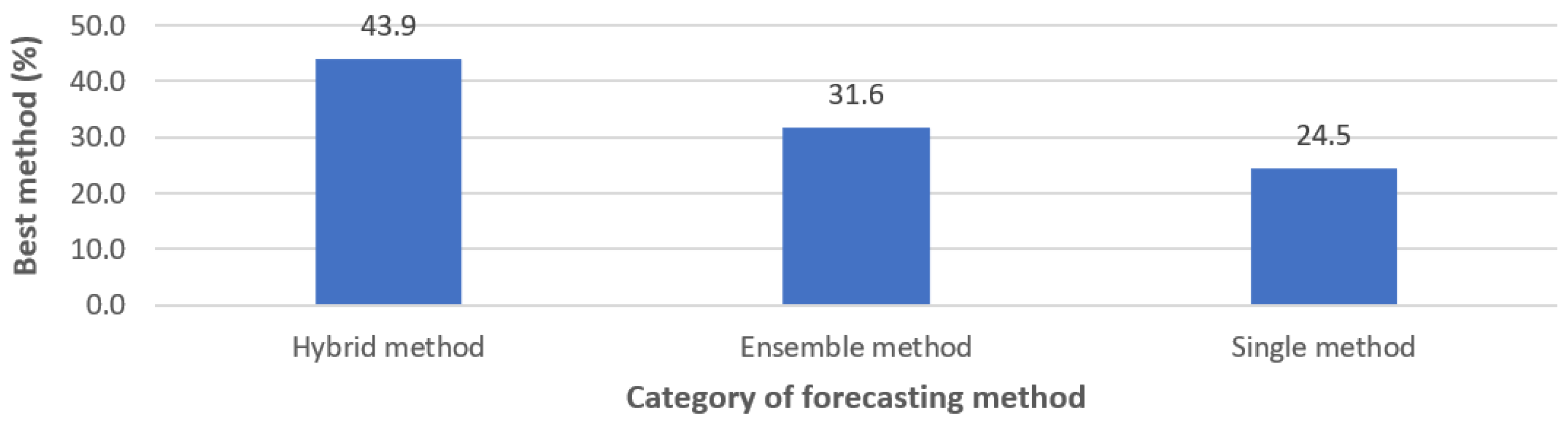
4.2.2. Analysis of Errors and EDF Depending on the Class of Forecasting Methods
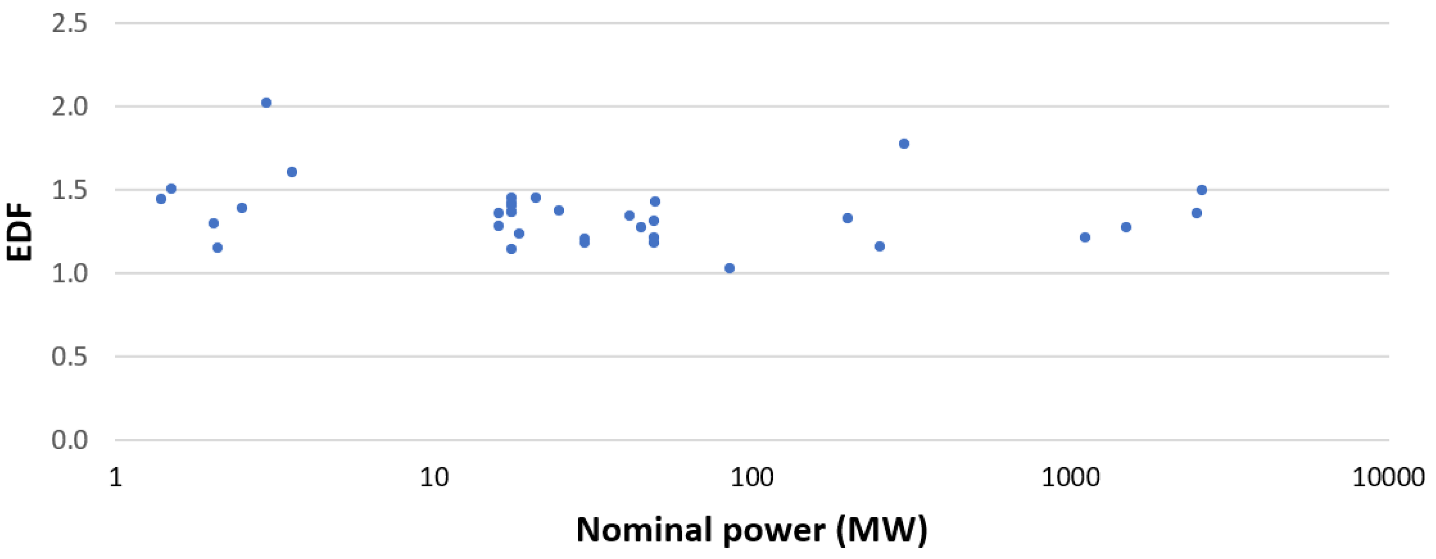
4.2.3. Analysis of Errors Based on System Size
4.2.4. Analysis of Error Based on System Location (Onshore v. Offshore)
5. Discussion
- mandatory use of normalized error metrics for the assessment of forecasting quality: nRMSE Formula (5) and nMAE Formula (6), accompanied by a description of the normalization method (recommended normalization using the rated power of the system), which would enable comparative assessments of the quality of studies of systems of various sizes (or regardless of how big the wind farm is);
- we do not recommend the use of MAPE metric, which is susceptible to substantial error for small or zero generations;
- mandatory use of a forecast conducted by naive (persistence) method to enable the assessment of the quality of the best model proposed by the authors of the paper relative to the reference model; in such case calculation of the skill score metric by Formula (17), (18), or (19) is recommended in addition;
- provide strict, precise information on forecasting horizon(s) and information if the forecast is, e.g., “One Step,” e.g., from 1 h to 24 h, or one step ahead with follow-up predictions (in which case forecasting errors are typically smaller);
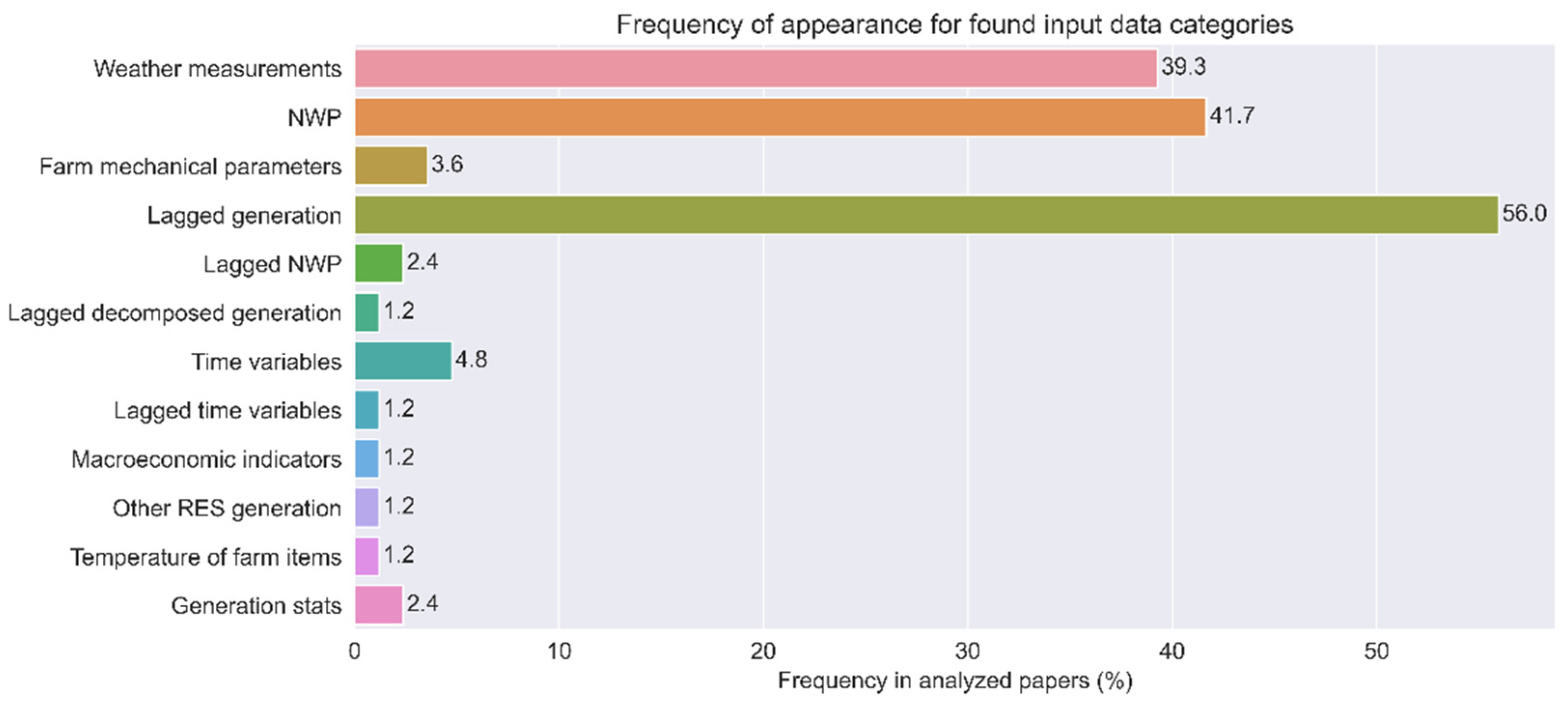
- provide strict, precise information on the set(s) of input data for the proposed model(s);
- provide the source of meteo forecasts (GFS, ECMWF, other sources) if used in the forecasting model;
- explicit statement on whether the forecasting model uses meteo forecasts and/or on-site measurements of weather conditions at the wind farm;
- provide the range of training, validation, and testing data, and how the range of data is divided into the identified subsets;
- provide details of the location, unless confidential (location and size of the wind farm, and landscape features prevalent at the location).
6. Conclusions
Author Contributions
Funding
Institutional Review Board Statement
Informed Consent Statement
Data Availability Statement
Conflicts of Interest
Abbreviations
| ANN | Artificial Neural Network |
| ARIMA | Autoregressive Integrated Moving Average |
| BP | Back Propagation |
| BPNN | BP Neural Network |
| CNN | Convolutional Neural Network |
| CSA | Crow Search Algorithm |
| DA | Dragonfly Algorithm |
| DBN | Deep Belief Network |
| DBSCAN | Density-Based Spatial Clustering of Applications with Noise |
| DGF | Double Gaussian Function |
| DWT | Discrete Wavelet Transform |
| EDCNN | Efficient Deep Convolution Neural Network |
| EDF | Error Dispersion Factor |
| EEMD | Ensemble Empirical Mode Decomposition |
| EMD | Empirical Mode Decomposition |
| EWT | Empirical Wavelet Transformation |
| FS | Feature Selection |
| GBT | Gradient Boosted Trees |
| GRU | Gated Recurrent Unit |
| HLNN | Laguerre Neural Network |
| HNN | Hybrid Neural Network |
| IPSO | Improved Particle Swarm Optimization |
| KNNR | K-Nearest Neighbors Regression |
| LD | Lorenz Disturbance System |
| LR | Linear Regression |
| LSTM | Long-Short-Term Memory |
| MAAPE | Mean Arctangent Absolute Percentage Error |
| MAE | Mean Absolute Error |
| MAPE | Mean Absolute Percentage Error |
| MBE | Mean Bias Error |
| MCC | Maximum Correntropy Criterion |
| MKRPINN | Multi-Kernel Regularized Pseudo Inverse Neural Network |
| MPSO | Modified Particle Swarm Optimization |
| MRE | Mean Relative Error |
| mRMR | Maximum Relevance and Minimum Redundancy Algorithm |
| MSE | Mean Squared Error |
| nMAE | Normalized Mean Absolute Error |
| NN | Neural Network |
| nRMSE | Normalized Root Mean Squared Error |
| NWP | Numerical Weather Prediction |
| OMS-QL | Online Model Selection using Q-learning |
| P | Promoting Percentages |
| PCA | Principal Component Analysis |
| PICP | Prediction Interval Coverage Probability |
| PINAW | Prediction Interval Normalized Average Width |
| PSO | Particle Swarm Optimization |
| R or CC | Pearson Linear Correlation Coefficient |
| R2 | R-square or Coefficient of Determination |
| RBF | Radial Basis Function |
| RES | Renewable Energy Sources |
| RF | Random Forest |
| RMSE | Root Mean Square Error |
| SAE | Stacked Auto-Encoders |
| SE | Sample Entropy |
| sMAPE | Symmetric Mean Absolute Percentage Error |
| SS | Skill Score |
| SSA | Singular Spectrum Analysis |
| STA | State Transition Algorithm |
| SVM | Support Vector Machine |
| SVR | Support Vector Regression |
| TIC | Theil’s Inequality Coefficient |
| VMD | Variational Mode Decomposition |
| WF | Wind Farm |
| WIPSO | Weight Improved Particle Swarm Optimization |
| WPT | Wavelet Packet Transform |
| WT | Wavelet Transform |
| xGBoost | eXtreme Gradient Boost |
References
- Piotrowski, P.; Kopyt, M.; Baczyński, D.; Robak, S.; Gulczynski, T. Hybrid and Ensemble Methods of Two Days Ahead Forecasts of Electric Energy Production in a Small Wind Turbine. Energies 2021, 14, 1225. [Google Scholar] [CrossRef]
- Piotrowski, P.; Baczyński, D.; Kopyt, M.; Gulczyński, T. Advanced Ensemble Methods Using Machine Learning and Deep Learning for One-Day-Ahead Forecasts of Electric Energy Production in Wind Farms. Energies 2022, 15, 1252. [Google Scholar] [CrossRef]
- Wang, Y.; Zou, R.; Liu, F.; Zhang, L.; Liu, Q. A review of wind speed and wind power forecasting with deep neural networks. Appl. Energy 2021, 304, 117766. [Google Scholar] [CrossRef]
- Hanifi, S.; Liu, X.; Lin, Z.; Lotfian, S. A Critical Review of Wind Power Forecasting Methods-Past, Present and Future. Energies 2020, 13, 3764. [Google Scholar] [CrossRef]
- Santhosh, M.; Venkaiah, C.; Vinod Kumar, D. Current advances and approaches in wind speed and wind power forecasting for improved renewable energy integration: A review. Eng. Rep. 2020, 2, e12178. [Google Scholar] [CrossRef]
- González-Sopeña, J.; Pakrashi, V.; Ghosh, B. An overview of performance evaluation metrics for short-term statistical wind power forecasting. Renew. Sustain. Energy Rev. 2021, 138, 110515. [Google Scholar] [CrossRef]
- Nazir, M.S.; Alturise, F.; Alshmrany, S.; Nazir, H.M.J.; Bilal, M.; Abdalla, A.N.; Sanjeevikumar, P.; Ali, Z.M. Wind Generation Forecasting Methods and Proliferation of Artificial Neural Network: A Review of Five Years Research Trend. Sustainability 2020, 12, 3778. [Google Scholar] [CrossRef]
- Tawn, R.; Browell, J. A review of very short-term wind and solar power forecasting. Renew. Sustain. Energy Rev. 2022, 153, 111758. [Google Scholar] [CrossRef]
- Chen, C.; Liu, H. Medium-term wind power forecasting based on multi-resolution multi-learner ensemble and adaptive model selection. Energy Convers. Manag. 2020, 206, 112492. [Google Scholar] [CrossRef]
- Mishra, S.P.; Dash, P.K. Short-term prediction of wind power using a hybrid pseudo-inverse Legendre neural network and adaptive firefly algorithm. Neural Comput. Appl. 2019, 31, 2243–2268. [Google Scholar] [CrossRef]
- Wang, H.; Liu, Y.; Zhou, B.; Li, C.; Cao, G.; Voropai, N.; Barakhtenko, E. Taxonomy research of artificial intelligence for deterministic solar power forecasting. Energy Convers. Manag. 2020, 214, 112909. [Google Scholar] [CrossRef]
- Piotrowski, P.; Baczyński, D.; Kopyt, M.; Szafranek, K.; Helt, P.; Gulczyński, T. Analysis of forecasted meteorological data (NWP) for efficient spatial forecasting of wind power generation. Electr. Power Syst. Res. 2019, 175, 105891. [Google Scholar] [CrossRef]
- Piotrowski, P.; Parol, M.; Kapler, P.; Fetliński, B. Advanced Forecasting Methods of 5-Minute Power Generation in a PV System for Microgrid Operation Control. Energies 2022, 15, 2645. [Google Scholar] [CrossRef]
- Yousuf, M.U.; Al-Bahadly, I.; Avci, E. Current Perspective on the Accuracy of Deterministic Wind Speed and Power Forecasting. IEEE Access 2019, 7, 159547–159564. [Google Scholar] [CrossRef]
- Mujeeb, S.; Alghamdi, T.A.; Ullah, S.; Fatima, A.; Javaid, N.; Saba, T. Exploiting Deep Learning for Wind Power Forecasting Based on Big Data Analytics. Appl. Sci. 2019, 9, 4417. [Google Scholar] [CrossRef]
- Wang, K.; Qi, X.; Liu, H.; Song, J. Deep belief network based k-means cluster approach for short-term wind power forecasting. Energy 2018, 165, 840–852. [Google Scholar] [CrossRef]
- Li, L.L.; Zhao, X.; Tseng, M.L.; Tan, R.R. Short-term wind power forecasting based on support vector machine with improved dragonfly algorithm. J. Clean. Prod. 2020, 242, 118447. [Google Scholar] [CrossRef]
- Lopez, E.; Valle, C.; Allende, H.; Gil, E.; Madsen, H. Wind Power Forecasting Based on Echo State Networks and Long ShortTerm Memory. Energies 2018, 11, 526. [Google Scholar] [CrossRef]
- Niu, Z.; Yu, Z.; Tang, W.; Wu, Q.; Reformat, M. Wind power forecasting using attention-based gated recurrent unit network. Energy 2020, 196, 117081. [Google Scholar] [CrossRef]
- Lin, Z.; Liu, X. Wind power forecasting of an offshore wind turbine based on high-frequency SCADA data and deep learning neural network. Energy 2020, 201, 117693. [Google Scholar] [CrossRef]
- Kisvari, A.; Lin, Z.; Liu, X. Wind power forecasting A data-driven method along with gated recurrent neural network. Renew. Energy 2021, 163, 1895–1909. [Google Scholar] [CrossRef]
- Ju, Y.; Sun, G.; Chen, Q.; Zhang, M.; Zhu, H.; Rehman, M.U. A Model Combining Convolutional Neural Network and LightGBM Algorithm for Ultra-Short-Term Wind Power Forecasting. IEEE Access 2019, 7, 28309–28318. [Google Scholar] [CrossRef]
- Demolli, H.; Dokuz, A.S.; Ecemis, A.; Gokcek, M. Wind power forecasting based on daily wind speed data using machine learning algorithms. Energy Convers. Manag. 2019, 198, 111823. [Google Scholar] [CrossRef]
- Yin, H.; Ou, Z.; Huang, S.; Meng, A. A cascaded deep learning wind power prediction approach based on a two-layer of mode decomposition. Energy 2019, 189, 116316. [Google Scholar] [CrossRef]
- Higashiyama, K.; Fujimoto, Y.; Hayashi, Y. Feature Extraction of NWP Data for Wind Power Forecasting Using 3D-Convolutional Neural Networks. Energy Procedia 2018, 155, 350–358. [Google Scholar] [CrossRef]
- Pan, J.S.; Hu, P.; Chu, S.C. Novel Parallel Heterogeneous Meta-Heuristic and Its Communication Strategies for the Prediction of Wind Power. Processes 2019, 7, 845. [Google Scholar] [CrossRef]
- Cali, U.; Sharma, V. Short-term wind power forecasting using long-short term memory based recurrent neural network model and variable selection. Int. J. Smart Grid Clean Energy 2019, 8, 103–110. [Google Scholar] [CrossRef]
- Jiang, P.; Li, R.; Li, H. Multi-objective algorithm for the design of prediction intervals for wind power forecasting model. Appl. Math. Model. 2019, 67, 101–122. [Google Scholar] [CrossRef]
- Sun, M.; Feng, C.; Zhang, J. Multi-distribution ensemble probabilistic wind power forecasting. Renew. Energy 2020, 148, 135–149. [Google Scholar] [CrossRef]
- Du, P. Ensemble Machine Learning-Based Wind Forecasting to Combine NWP Output with Data from Weather Station. IEEE Trans. Sustain. Energy 2019, 10, 2133–2141. [Google Scholar] [CrossRef]
- Wang, C.; Zhang, H.; Ma, P. Wind power forecasting based on singular spectrum analysis and a new hybrid Laguerre neural network. Appl. Energy 2020, 259, 114139. [Google Scholar] [CrossRef]
- Wang, Z.; Zhang, J.; Zhang, Y.; Huang, C.; Wang, L. Short-Term Wind Speed Forecasting Based on Information of Neighboring Wind Farms. IEEE Access 2020, 8, 16760–16770. [Google Scholar] [CrossRef]
- Sun, Z.; Zhao, S.; Zhang, J. Short-Term Wind Power Forecasting on Multiple Scales Using VMD Decomposition, K-Means Clustering and LSTM Principal Computing. IEEE Access 2019, 7, 166917–166929. [Google Scholar] [CrossRef]
- Nourani Esfetang, N.; Kazemzadeh, R. A novel hybrid technique for prediction of electric power generation in wind farms based on WIPSO, neural network and wavelet transform. Energy 2018, 149, 662–674. [Google Scholar] [CrossRef]
- Du, P.; Wang, J.; Yang, W.; Niu, T. A novel hybrid model for short-term wind power forecasting. Appl. Soft Comput. 2019, 80, 93–106. [Google Scholar] [CrossRef]
- Hu, H.; Wang, L.; Lv, S.X. Forecasting energy consumption and wind power generation using deep echo state network. Renew. Energy 2020, 154, 598–613. [Google Scholar] [CrossRef]
- Yildiz, C.; Acikgoz, H.; Korkmaz, D.; Budak, U. An improved residual-based convolutional neural network for very short-term wind power forecasting. Energy Convers. Manag. 2021, 228, 113731. [Google Scholar] [CrossRef]
- Zheng, H.; Wu, Y. A XGBoost Model with Weather Similarity Analysis and Feature Engineering for Short-Term Wind Power Forecasting. Appl. Sci. 2019, 9, 3019. [Google Scholar] [CrossRef]
- Bhatt, G.A.; Gandhi, P.R. Statistical and ANN based prediction of wind power with uncertainty. In Proceedings of the 3rd International Conference on Trends in Electronics and Informatics (ICOEI), Tirunelveli, India, 23–25 April 2019; pp. 622–627. [Google Scholar] [CrossRef]
- Shahid, F.; Zameer, A.; Mehmood, A.; Raja, M.A.Z. A novel wavenets long short term memory paradigm for wind power prediction. Appl. Energy 2020, 269, 115098. [Google Scholar] [CrossRef]
- Dong, W.; Yang, Q.; Fang, X. Multi-Step Ahead Wind Power Generation Prediction Based on Hybrid Machine Learning Techniques. Energies 2018, 11, 1975. [Google Scholar] [CrossRef]
- Hong, Y.Y.; Rioflorido, C.L.P.P. A hybrid deep learning-based neural network for 24-h ahead wind power forecasting. Appl. Energy 2019, 250, 530–539. [Google Scholar] [CrossRef]
- Zhang, Y.; Chen, B.; Zhao, Y.; Pan, G. Wind Speed Prediction of IPSO-BP Neural Network Based on Lorenz Disturbance. IEEE Access 2018, 6, 53168–53179. [Google Scholar] [CrossRef]
- Naik, J.; Dash, S.; Dash, P.; Bisoi, R. Short term wind power forecasting using hybrid variational mode decomposition and multi-kernel regularized pseudo inverse neural network. Renew. Energy 2018, 118, 180–212. [Google Scholar] [CrossRef]
- Zhang, C.; Peng, T.; Nazir, M.S. A novel hybrid approach based on variational heteroscedastic Gaussian process regression for multi-step ahead wind speed forecasting. Int. J. Electr. Power Energy Syst. 2022, 136, 107717. [Google Scholar] [CrossRef]
- Shen, Y.; Wang, X.; Chen, J. Wind Power Forecasting Using Multi-Objective Evolutionary Algorithms for Wavelet Neural Network-Optimized Prediction Intervals. Appl. Sci. 2018, 8, 185. [Google Scholar] [CrossRef]
- Yuan, X.; Chen, C.; Jiang, M.; Yuan, Y. Prediction interval of wind power using parameter optimized Beta distribution based LSTM model. Appl. Soft Comput. 2019, 82, 105550. [Google Scholar] [CrossRef]
- Li, R.; Jin, Y. A wind speed interval prediction system based on multi-objective optimization for machine learning method. Appl. Energy 2018, 228, 2207–2220. [Google Scholar] [CrossRef]
- Qin, G.; Yan, Q.; Zhu, J.; Xu, C.; Kammen, D.M. Day-Ahead Wind Power Forecasting Based on Wind Load Data Using Hybrid Optimization Algorithm. Sustainability 2021, 13, 1164. [Google Scholar] [CrossRef]
- Duan, J.; Wang, P.; Ma, W.; Tian, X.; Fang, S.; Cheng, Y.; Chang, Y.; Liu, H. Short-term wind power forecasting using the hybrid model of improved variational mode decomposition and Correntropy Long Short-term memory neural network. Energy 2021, 214, 118980. [Google Scholar] [CrossRef]
- Li, N.; He, F.; Ma, W. Wind Power Prediction Based on Extreme Learning Machine with Kernel Mean p-Power Error Loss. Energies 2019, 12, 673. [Google Scholar] [CrossRef]
- Amila, T.; Peiris, J.J.; Rathnayake, U. Forecasting Wind Power Generation Using Artificial Neural Network: “Pawan Danawi” A Case Study from Sri Lanka. J. Electr. Comput. Eng. 2021, 2021, 5577547. [Google Scholar] [CrossRef]
- Fu, Y.; Hu, W.; Tang, M.; Yu, R.; Liu, B. Multi-step Ahead Wind Power Forecasting Based on Recurrent Neural Networks. In Proceedings of the IEEE PES Asia-Pacific Power and Energy Engineering Conference (APPEEC), Kota Kinabalu, Malaysia, 7–8 October 2018; pp. 217–222. [Google Scholar] [CrossRef]
- Liu, H.; Mi, X.W.; Li, Y.F. Wind speed forecasting method based on deep learning strategy using empirical wavelet transform, long short term memory neural network and Elman neural network. Energy Convers. Manag. 2018, 156, 498–514. [Google Scholar] [CrossRef]
- Zhou, J.; Xu, X.; Huo, X.; Li, Y. Forecasting Models for Wind Power Using Extreme-Point Symmetric Mode Decomposition and Artificial Neural Networks. Sustainability 2019, 11, 650. [Google Scholar] [CrossRef]
- Bazionis, I.K.; Georgilakis, P.S. Review of Deterministic and Probabilistic Wind Power Forecasting: Models, Methods, and Future Research. Electricity 2021, 2, 13–47. [Google Scholar] [CrossRef]
- Jiao, R.; Huang, X.; Ma, X.; Han, L.; Tian, W. A Model Combining Stacked Auto Encoder and Back Propagation Algorithm for Short-Term Wind Power Forecasting. IEEE Access 2018, 6, 17851–17858. [Google Scholar] [CrossRef]
- Ding, M.; Zhou, H.; Xie, H.; Wu, M.; Nakanishi, Y.; Yokoyama, R. A gated recurrent unit neural networks based wind speed error correction model for short-term wind power forecasting. Neurocomputing 2019, 365, 54–61. [Google Scholar] [CrossRef]
- Wang, S.X.; Li, M.; Zhao, L.; Jin, C. Short-term wind power prediction based on improved small-world neural network. Neural Comput. Appl. 2019, 31, 3173–3185. [Google Scholar] [CrossRef]
- Torabi, A.; Mousavy, S.A.K.; Dashti, V.; Saeedi, M.; Yousefi, N. A New Prediction Model Based on Cascade NN for Wind Power Prediction. Comput. Econ. 2019, 53, 1219–1243. [Google Scholar] [CrossRef]
- Memarzadeh, G.; Keynia, F. A new short-term wind speed forecasting method based on fine-tuned LSTM neural network and optimal input sets. Energy Convers. Manag. 2020, 213, 112824. [Google Scholar] [CrossRef]
- Shivani; Sandhu, K.; Ramachandran Nair, A. A Comparative Study of ARIMA and RNN for Short Term Wind Speed Forecasting. In Proceedings of the 10th International Conference on Computing, Communication and Networking Technologies (ICCCNT), Kanpur, India, 6–8 July 2019; pp. 1–7. [Google Scholar] [CrossRef]
- Sopena, J.M.G.; Pakrashi, V.; Ghosh, B. Can we improve short-term wind power forecasts using turbine-level data? A case study in Ireland. In Proceedings of the IEEE Madrid PowerTech, Madrid, Spain, 28 June–2 July 2021; pp. 1–6. [Google Scholar] [CrossRef]
- Saini, V.K.; Kumar, R.; Mathur, A.; Saxena, A. Short term forecasting based on hourly wind speed data using deep learning algorithms. In Proceedings of the 3rd International Conference on Emerging Technologies in Computer Engineering: Machine Learning and Internet of Things (ICETCE), Jaipur, India, 7–8 February 2020; pp. 1–6. [Google Scholar] [CrossRef]
- Reddy, V.; Verma, S.M.; Verma, K.; Kumar, R. Hybrid Approach for Short Term Wind Power Forecasting. In Proceedings of the 9th International Conference on Computing, Communication and Networking Technologies (ICCCNT), Bengaluru, India, 10–12 July 2018; pp. 1–5. [Google Scholar] [CrossRef]
- Hu, T.; Wu, W.; Guo, Q.; Sun, H.; Shi, L.; Shen, X. Very short-term spatial and temporal wind power forecasting A deep learning approach. CSEE J. Power Energy Syst. 2020, 6, 434–443. [Google Scholar] [CrossRef]
- Karthikeyan, M.; Rengaraj, R. Short-Term Wind Speed Forecasting Using Ensemble Learning. In Proceedings of the 7th International Conference on Electrical Energy Systems (ICEES), Chennai, India, 11–13 February 2021; pp. 502–506. [Google Scholar] [CrossRef]
- Liu, Y.; Ghasemkhani, A.; Yang, L.; Zhao, J.; Zhang, J.; Vittal, V. Seasonal Self-evolving Neural Networks Based Short-term Wind Farm Generation Forecast. In Proceedings of the IEEE International Conference on Communications, Control, and Computing Technologies for Smart Grids (SmartGridComm), Tempe, AZ, USA, 11–13 November 2020; pp. 1–6. [Google Scholar] [CrossRef]
- Verma, S.M.; Reddy, V.; Verma, K.; Kumar, R. Markov Models Based Short Term Forecasting of Wind Speed for Estimating Day-Ahead Wind Power. In Proceedings of the International Conference on Power, Energy, Control and Transmission Systems (ICPECTS), Chennai, India, 22–23 February 2018; pp. 31–35. [Google Scholar] [CrossRef]
- Zhang, P.; Wang, Y.; Liang, L.; Li, X.; Duan, Q. Short-Term Wind Power Prediction Using GA-BP Neural Network Based on DBSCAN Algorithm Outlier Identification. Processes 2020, 8, 157. [Google Scholar] [CrossRef]
- Niu, D.; Pu, D.; Dai, S. Ultra-Short-Term Wind-Power Forecasting Based on the Weighted Random Forest Optimized by the Niche Immune Lion Algorithm. Energies 2018, 11, 1098. [Google Scholar] [CrossRef]
- Liu, Y.; Guan, L.; Hou, C.; Han, H.; Liu, Z.; Sun, Y.; Zheng, M. Wind Power Short-Term Prediction Based on LSTM and Discrete Wavelet Transform. Appl. Sci. 2019, 9, 1108. [Google Scholar] [CrossRef]
- Zhou, J.; Yu, X.; Jin, B. Short-Term Wind Power Forecasting: A New Hybrid Model Combined Extreme-Point Symmetric Mode Decomposition, Extreme Learning Machine and Particle Swarm Optimization. Sustainability 2018, 10, 3202. [Google Scholar] [CrossRef]
- Shi, X.; Lei, X.; Huang, Q.; Huang, S.; Ren, K.; Hu, Y. Hourly Day-Ahead Wind Power Prediction Using the Hybrid Model of Variational Model Decomposition and Long Short-Term Memory. Energies 2018, 11, 3227. [Google Scholar] [CrossRef]
- Wang, S.; Zhao, X.; Li, M.; Wang, H. TRSWA-BP Neural Network for Dynamic Wind Power Forecasting Based on Entropy Evaluation. Entropy 2018, 20, 284. [Google Scholar] [CrossRef]
- An, G.; Jiang, Z.; Chen, L.; Cao, X.; Li, Z.; Zhao, Y.; Sun, H. Ultra Short-Term Wind Power Forecasting Based on Sparrow Search Algorithm Optimization Deep Extreme Learning Machine. Sustainability 2021, 13, 10453. [Google Scholar] [CrossRef]
- Donadio, L.; Fang, J.; Porté-Agel, F. Numerical Weather Prediction and Artificial Neural Network Coupling for Wind Energy Forecast. Energies 2021, 14, 338. [Google Scholar] [CrossRef]
- Kosana, V.; Teeparthi, K.; Madasthu, S.; Kumar, S. A novel reinforced online model selection using Q-learning technique for wind speed prediction. Sustain. Energy Technol. Assess. 2022, 49, 101780. [Google Scholar] [CrossRef]
- Duan, J.; Wang, P.; Ma, W.; Fang, S.; Hou, Z. A novel hybrid model based on nonlinear weighted combination for short-term wind power forecasting. Int. J. Electr. Power Energy Syst. 2022, 134, 107452. [Google Scholar] [CrossRef]
- Xiang, L.; Liu, J.; Yang, X.; Hu, A.; Su, H. Ultra-short term wind power prediction applying a novel model named SATCN-LSTM. Energy Convers. Manag. 2022, 252, 115036. [Google Scholar] [CrossRef]
- Hanifi, S.; Lotfian, S.; Seyedzadeh, S.; Zare-Behtash, H.; Cammarano, A. Offshore wind power forecasting—A new hyperparameter optimisation algorithm for deep learning models. Energies 2022, 15, 6919. [Google Scholar] [CrossRef]
- Farah, S.; David, A.W.; Humaira, N.; Aneela, Z.; Steffen, E. Short-term multi-hour ahead country-wide wind power prediction for Germany using gated recurrent unit deep learning. Renew. Sustain. Energy Rev. 2022, 167, 112700. [Google Scholar] [CrossRef]
- Kosovic, B.; Haupt, S.E.; Adriaansen, D.; Alessandrini, S.; Wiener, G.; Delle Monache, L.; Liu, Y.; Linden, S.; Jensen, T.; Cheng, W.; et al. A Comprehensive Wind Power Forecasting System Integrating Artificial Intelligence and Numerical Weather Prediction. Energies 2020, 13, 1372. [Google Scholar] [CrossRef]
- Yu, R.; Gao, J.; Yu, M.; Lu, W.; Xu, T.; Zhao, M.; Zhang, J.; Zhang, R.; Zhang, Z. LSTM-EFG for wind power forecasting based on sequential correlation features. Future Gener. Comput. Syst. 2019, 93, 33–42. [Google Scholar] [CrossRef]
- Yu, R.; Liu, Z.; Li, X.; Lu, W.; Ma, D.; Yu, M.; Wang, J.; Li, B. Scene learning: Deep convolutional networks for wind power prediction by embedding turbines into grid space. Appl. Energy 2019, 238, 249–257. [Google Scholar] [CrossRef]
- Oh, E.; Wang, H. Reinforcement-Learning-Based Energy Storage System Operation Strategies to Manage Wind Power Forecast Uncertainty. IEEE Access 2020, 8, 20965–20976. [Google Scholar] [CrossRef]
- Wang, X.; Li, P.; Yang, J. Short-term Wind Power Forecasting Based on Two-stage Attention Mechanism. IET Renew. Power Gener. 2019, 14, 297–304. [Google Scholar] [CrossRef]
- Dorado-Moreno, M.; Navarin, N.; Gutierrez, P.; Prieto, L.; Sperduti, A.; Salcedo-Sanz, S.; Hervas-Martinez, C. Multi-task learning for the prediction of wind power ramp events with deep neural networks. Neural Netw. 2020, 123, 401–411. [Google Scholar] [CrossRef]
- Ma, Y.J.; Zhai, M.Y. A Dual-Step Integrated Machine Learning Model for 24h-Ahead Wind Energy Generation Prediction Based on Actual Measurement Data and Environmental Factors. Appl. Sci. 2019, 9, 2125. [Google Scholar] [CrossRef]
- Khosravi, A.; Machado, L.; Nunes, R. Time-series prediction of wind speed using machine learning algorithms: A case study Osorio wind farm, Brazil. Appl. Energy 2018, 224, 550–566. [Google Scholar] [CrossRef]
- Wang, R.; Li, C.; Fu, W.; Tang, G. Deep Learning Method Based on Gated Recurrent Unit and Variational Mode Decomposition for Short-Term Wind Power Interval Prediction. IEEE Trans. Neural Netw. Learn. Syst. 2020, 31, 3814–3827. [Google Scholar] [CrossRef] [PubMed]
- Han, L.; Jing, H.; Zhang, R.; Gao, Z. Wind power forecast based on improved Long Short Term Memory network. Energy 2019, 189, 116300. [Google Scholar] [CrossRef]
- Sharifian, A.; Ghadi, M.J.; Ghavidel, S.; Li, L.; Zhang, J. A new method based on Type-2 fuzzy neural network for accurate wind power forecasting under uncertain data. Renew. Energy 2018, 120, 220–230. [Google Scholar] [CrossRef]
- He, Y.; Li, H. Probability density forecasting of wind power using quantile regression neural network and kernel density estimation. Energy Convers. Manag. 2018, 164, 374–384. [Google Scholar] [CrossRef]
- Shao, H.; Deng, X.; Jiang, Y. A novel deep learning approach for short-term wind power forecasting based on infinite feature selection and recurrent neural network. J. Renew. Sustain. Energy 2018, 10, 043303. [Google Scholar] [CrossRef]
- Dong, D.; Sheng, Z.; Yang, T. Wind Power Prediction Based on Recurrent Neural Network with Long Short-Term Memory Units. In Proceedings of the 2018 International Conference on Renewable Energy and Power Engineering (REPE), Toronto, ON, Canada, 24–26 November 2018; pp. 34–38. [Google Scholar] [CrossRef]
- Yang, X.; Zhang, Y.; Yang, Y.; Lv, W. Deterministic and Probabilistic Wind Power Forecasting Based on Bi-Level Convolutional Neural Network and Particle Swarm Optimization. Appl. Sci. 2019, 9, 1794. [Google Scholar] [CrossRef]
- Ak, R.; Li, Y.F.; Vitelli, V.; Zio, E. Adequacy assessment of a wind-integrated system using neural network-based interval predictions of wind power generation and load. Int. J. Electr. Power Energy Syst. 2018, 95, 213–226. [Google Scholar] [CrossRef]
- Sun, G.; Jiang, C.; Cheng, P.; Liu, Y.; Wang, X.; Fu, Y.; He, Y. Short-term wind power forecasts by a synthetical similar time series data mining method. Renew. Energy 2018, 115, 575–584. [Google Scholar] [CrossRef]
- Sitharthan, R.; Parthasarathy, T.; Sheeba Rani, S.; Ramya, K.C. An improved radial basis function neural network control strategy-based maximum power point tracking controller for wind power generation system. Trans. Inst. Meas. Control 2019, 41, 3158–3170. [Google Scholar] [CrossRef]
- Abedinia, O.; Lotfi, M.; Bagheri, M.; Sobhani, B.; Shafiekhah, M.; Catalao, J.P.S. Improved EMD-Based Complex Prediction Model for Wind Power Forecasting. IEEE Trans. Sustain. Energy 2020, 11, 2790–2802. [Google Scholar] [CrossRef]
- Hammerschmitt, B.; Lucchese, F.C.; Silva, L.N.; Abaide, A.R.; Rohr, J.A.D.A. Short-Term Generation Forecasting Against the High Penetration of the Wind Energy. In Proceedings of the 8th International Conference on Modern Power Systems (MPS), Cluj-Napoca, Romania, 21–23 May 2019; pp. 1–6. [Google Scholar] [CrossRef]
- Abesamis, K.; Ang, P.; Bisquera, F.I.; Catabay, G.; Tindogan, P.; Ostia, C.; Pacis, M. Short-Term Wind Power Forecasting Using Structured Neural Network. In Proceedings of the IEEE 11th International Conference on Humanoid, Nanotechnology, Information Technology, Communication and Control, Environment, and Management (HNICEM), Laoag, Philippines, 29 November–1 December 2019; pp. 1–4. [Google Scholar] [CrossRef]
- Bhushan Sahay, K.; Srivastava, S. Short-Term Wind Speed Forecasting of Lelystad Wind Farm by Using ANN Algorithms. In Proceedings of the International Electrical Engineering Congress (iEECON), Krabi, Thailand, 7–9 March 2018; pp. 1–4. [Google Scholar] [CrossRef]
- Vaitheeswaran, S.S.; Ventrapragada, V.R. Wind Power Pattern Prediction in time series measuremnt data for wind energy prediction modelling using LSTM-GA networks. In Proceedings of the 10th International Conference on Computing, Communication and Networking Technologies (ICCCNT), Kanpur, India, 6–8 July 2019; pp. 1–5. [Google Scholar] [CrossRef]
- Wang, S.; Sun, Y.; Zhai, S.; Hou, D.; Wang, P.; Wu, X. Ultra-Short-Term Wind Power Forecasting Based on Deep Belief Network. In Proceedings of the Chinese Control Conference (CCC), Guangzhou, China, 27–30 July 2019; pp. 7479–7483. [Google Scholar] [CrossRef]
- Medina, S.V.; Ajenjo, U.P. Performance Improvement of Artificial Neural Network Model in Short-term Forecasting of Wind Farm Power Output. J. Mod. Power Syst. Clean Energy 2020, 8, 484–490. [Google Scholar] [CrossRef]
- Pang, D.; Li, G. Research on Wind Power Output Reconstruction Technology Based on Multiple Time Scales. In Proceedings of the 2nd IEEE Conference on Energy Internet and Energy System Integration (EI2), Beijing, China, 20–22 October 2018; pp. 1–5. [Google Scholar] [CrossRef]
- Prabha, P.P.; Vanitha, V.; Resmi, R. Wind Speed Forecasting using Long Short Term Memory Networks. In Proceedings of the 2019 2nd International Conference on Intelligent Computing, Instrumentation and Control Technologies (ICICICT), Kannur, India, 5–6 July 2019; Volume 1, pp. 1310–1314. [Google Scholar] [CrossRef]
- Musbah, H.; Aly, H.H.; Little, T.A. A Novel Approach for Seasonality and Trend Detection using Fast Fourier Transform in Box-Jenkins Algorithm. In Proceedings of the IEEE Canadian Conference on Electrical and Computer Engineering (CCECE), London, ON, Canada, 30 August–2 September 2020; pp. 1–5. [Google Scholar] [CrossRef]
- Viet, D.T.; Phuong, V.V.; Duong, M.Q.; Tran, Q.T. Models for Short-Term Wind Power Forecasting Based on Improved Artificial Neural Network Using Particle Swarm Optimization and Genetic Algorithms. Energies 2020, 13, 2873. [Google Scholar] [CrossRef]
- Liu, T.; Huang, Z.; Tian, L.; Zhu, Y.; Wang, H.; Feng, S. Enhancing Wind Turbine Power Forecast via Convolutional Neural Network. Electronics 2021, 10, 261. [Google Scholar] [CrossRef]
- Tang, B.; Chen, Y.; Chen, Q.; Su, M. Research on Short-Term Wind Power Forecasting by Data Mining on Historical Wind Resource. Appl. Sci. 2020, 10, 1295. [Google Scholar] [CrossRef]
- Liu, B.; Zhao, S.; Yu, X.; Zhang, L.; Wang, Q. A Novel Deep Learning Approach for Wind Power Forecasting Based on WD-LSTM Model. Energies 2020, 13, 4964. [Google Scholar] [CrossRef]
- Bochenek, B.; Jurasz, J.; Jaczewski, A.; Stachura, G.; Sekuła, P.; Strzyżewski, T.; Wdowikowski, M.; Figurski, M. Day-Ahead Wind Power Forecasting in Poland Based on Numerical Weather Prediction. Energies 2021, 14, 2164. [Google Scholar] [CrossRef]
- Li, Y.; Yang, F.; Zha, W.; Yan, L. Combined Optimization Prediction Model of Regional Wind Power Based on Convolution Neural Network and Similar Days. Machines 2020, 8, 80. [Google Scholar] [CrossRef]
- Gouveia, H.T.V.; De Aquino, R.R.B.; Ferreira, A.A. Enhancing Short-Term Wind Power Forecasting through Multiresolution Analysis and Echo State Networks. Energies 2018, 11, 824. [Google Scholar] [CrossRef]
- Ahmadi, A.; Nabipour, M.; Mohammadi-Ivatloo, B.; Amani, A.M.; Rho, S.; Piran, M.J. Long-Term Wind Power Forecasting Using Tree-Based Learning Algorithms. IEEE Access 2020, 8, 151511–151522. [Google Scholar] [CrossRef]
- Liu, H.; Chen, C.; Lv, X.; Wu, X.; Liu, M. Deterministic wind energy forecasting: A review of intelligent predictors and auxiliary methods. Energy Convers. Manag. 2019, 195, 328–345. [Google Scholar] [CrossRef]
- Al-Zadjali, S.; Al Maashri, A.; Al-Hinai, A.; Al Abri, R.; Gajare, S.; Al Yahyai, S.; Bakhtvar, M. A Fast and Accurate Wind Speed and Direction Nowcasting Model for Renewable Energy Management Systems. Energies 2021, 14, 7878. [Google Scholar] [CrossRef]
- Ding, C.; Zhou, Y.; Ding, Q.; Li, K. Integrated Carbon-Capture-Based Low-Carbon Economic Dispatch of Power Systems Based on EEMD-LSTM-SVR Wind Power Forecasting. Energies 2022, 15, 1613. [Google Scholar] [CrossRef]
- Yang, H.; Jiang, P.; Wang, Y.; Li, H. A fuzzy intelligent forecasting system based on combined fuzzification strategy and improved optimization algorithm for renewable energy power generation. Appl. Energy 2022, 325, 119849. [Google Scholar] [CrossRef]
- Madsen, H.; Pinson, P.; Kariniotakis, G.; Nielsen, H.A.; Nielsen, T.S. A Protocol for Standardazing the Performance Evaluation of Short Term Wind Power Prediction Models. Wind Eng. 2005, 29, 475–489. [Google Scholar] [CrossRef]
- Hyndman, R.J.; Koehler, A.B. Another Look at Measures of Forecast Accuracy. Int. J. Forecast. 2006, 22, 679–688. [Google Scholar] [CrossRef]


| Horizon | Applications | Duration |
|---|---|---|
| Very short-term | Turbine regulation, control strategies, electricity market billing, real-time grid operation, network stability, voltage control | 10 s |
| Short-term | Economic load dispatch planning, load amount, reversibility of power management, electric market reliability in day-ahead, load decisions for increments | 5 min, 10 min, 15 min, 1 h, 24 h |
| Medium-term | Unit commitment, reserved requirement, generation operator, operation scheduling | 1 month |
| Long-term | Maintenance scheduling, wind farm design, electricity market restructuring, optimization of operating costs | 1 month, 1 year |
| Factor | Description/Influence on Error Level |
|---|---|
| Time horizon | With increasing forecasting horizon, forecasting errors grow significantly, mainly due to the falling quality of NWP forecasts [5,6,8,10,11] |
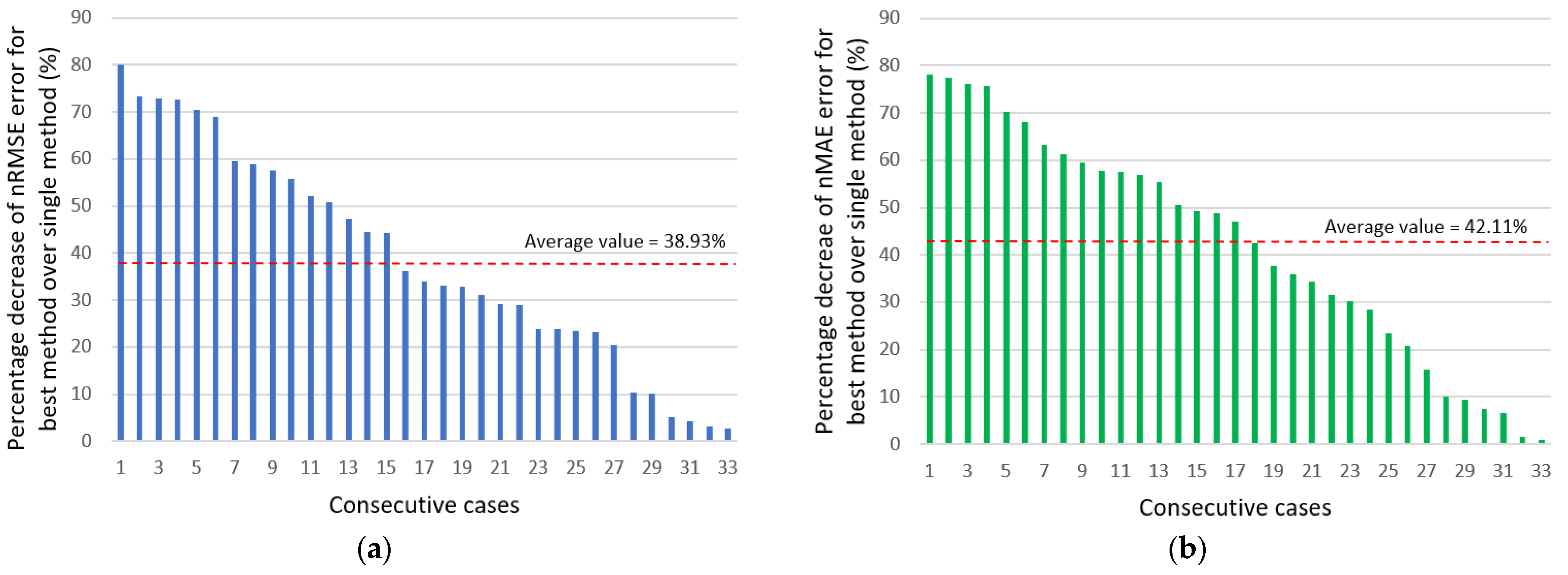
| Forecasting method (complexity) | Complex (ensemble or hybrid) models have typically lower forecasting errors than single methods (more details in Section 2) [1,2,3,4,5,8] |
| Size of system | The inertia of power production usually grows with system size. This translates into more predictable production, especially in shorter horizons. |
| Site (onshore/offshore) | Forecasting errors for offshore wind farms should be less than for onshore wind farms due to distinctive characteristics of weather conditions (more stable and higher wind speeds). |
| Landscape | Forecasting errors for farms located in rough terrain can depend on the local landscape and meteorological features (e.g., a forest, hills, or a lake in a direct neighborhood). The best if the terrain has as little roughness as possible—this guarantees the optimal generation of wind energy [12] |
| Location of NWP forecasting points | NWP forecasts from points more distant from the wind farm can generate larger forecasting errors. The topic of optimum selection of NWP forecasting points and their location on the farm is subject to studies [12] |
| Types and quantities of input data | The more information related to power generation can be used in the model, the more accurate generation forecasts can be expected. In particular, using NWP as input data is especially important (if absent, generation forecast errors grow very sharply), and with horizons of more than several hours, NWPs are virtually indispensable [1,2,4,13] |
| NWP data sources | NWP data can vary by quality (forecasting accuracy)—the more accurate NWP forecasts, the lower power generation forecasting error [2] |
| Quantity of training sets | The model must use training data encompassing at least one year. With a growing number of years, the model uses more information and better represents the seasonality and daily variability of the process (a smaller forecasting error can be expected) |
| Data preprocessing | Properly conducted steps to clean up and process raw input data can reduce forecasting error [3] |
| Data postprocessing | Elimination of impossible situations, e.g., negative power forecasts or forecasts determined as unlikely for specific input data. Elimination of such cases reduces the error [13] |
| Measurement data availability lag | Using up-to-date, current data provides for identification and correction of errors “on the fly,” e.g., using switchable forecasting models |
| Technique | Description | Advantage | Disadvantage |
|---|---|---|---|
| Naive/Persistence Methods | Simple approach that evaluates the last period t, benchmark for more complex methods | Fast results, applicable only for short-term forecasts | Does not consider correlations between input data and the results are not reliable for the subsequent steps in time |
| Physical Methods | Physical mathematical model of the power turbine | No need for training or historical data, enables understanding of physical behavior | Computationally complex, it relies on fresh data from several features, extensive setup effort |
| Statistical/Multivariate Methods (time series) | Mapping of relations between features, generally through recursive techniques, no NWP data as an input | Models can be built easily and with small computational effort | Quick loss of accuracy with time |
| AI/ML methods (LR, GBT, RF, BPNN, KNNR, LSTM, CNN, DBN, GRU, EDCNN, RBF, SVR) | Techniques that enable the computer to mimic human behavior without a predefined mathematical model (“black box”) | Highest accuracy and can learn more complex nonlinear relations | Slower convergence speed, risk of overfitting, computational complexity |
| Technique | Description | Advantage | Disadvantage |
|---|---|---|---|
| Ensemble methods | Aggregate a combination of results from different methods | Usually perform better than a single method | Larger computational cost of running individual methods; the combination of results can obscure problems inherent in the methods |
| Hybrid methods | Combination of different methods connected in series to create hybrid prediction structures. | Usually perform better than a single method | Larger computational cost of running individual methods; require large quantities of data |
| No. | Title/Reference | Horizon | System Nominal Power *** | Method Details | Error Metric | Input Data Details | |
|---|---|---|---|---|---|---|---|
| - | - | - | nRMSE | nMAE | - | ||
| 1. | Wind power forecasting based on daily wind speed data using machine learning algorithms [23] Proposed Method—--- | 1 year | 1 MW | RF (ensemble) | 0.0302 * | 0.0070 * | Daily wind speed, mean wind speed, standard deviation, total generated wind power values—Turkish State Meteorological Service |
| XGBoost (ensemble) | 0.0344 * | 0.0065 * | |||||
| 2. | Short-term wind power forecasting based on support vector machine with improved dragonfly algorithm [17] Proposed Method—IDA-SVM | 48 h | 2050 KW | IDA-SVM (hybrid) | 0.0524 | 0.0404 | Wind power, wind speed, wind direction, and temperature—La Haute Borne wind farm |
| DA-SVM (hybrid) | 0.0617 | 0.0515 | |||||
| 3. | A cascaded deep learning wind power prediction approach based on a two-layer of mode decomposition [24] Proposed Method—EMD-VMD-CNN-LSTM | 1, 2, 3 steps | ? MW | EMD-VMD-CNN-LSTM (Dataset #1, avg, hybrid) | 0.0329 * | 0.0227 * | Three sets of hourly averaged wind power, wind speed, and wind direction time series, Sotavento Galicia wind farm |
| EMD-VMD-CNN (Dataset #1, avg, hybrid) | 0.0396 * | 0.0321 * | |||||
| 4. | A Model Combining Stacked Auto Encoder and Back Propagation Algorithm for Short-Term Wind Power Forecasting [57] Proposed Method—SAE_BP | 1, 2, …, 9 steps | 1500 MW | SAE_BP (avg, hybrid/ensemble) | 0.0941 * | 0.0738 * | Wind generation from Ireland all island—EirGrid Group |
| SVM (avg, single) | 0.1396 * | 0.1185 * | |||||
| 5. | Deep belief network based k-means cluster approach for short-term wind power forecasting [16] Proposed Method—DBN | 10 min | 17.56 MW | DBN (single) | 0.0322 | 0.0236 | Wind speed, wind direction, temperature, humidity, pressure, history wind speed, history wind power—NWP meteogalicia and Sotavento wind farm |
| BP (single) | 0.0580 | 0.0446 | |||||
| 6. | Multi-distribution ensemble probabilistic wind power forecasting [29] Proposed Method—MDE | 1, 6, 24 h | 16 MW | Q-learning (6 h, single) | 0.2355 | 0.1841 | Meteorological information (many features), synthetic actual wind power, and wind power forecasts generated by the Weather Research and Forecasting (WRF) model—MDE probabilistic forecasting framework, from the Wind Integration National Dataset (WIND) Toolkit |
| NWP (24 h, single) | 0.1817 | 0.1337 | |||||
| 7. | Forecasting energy consumption and wind power generation using deep echo state network [36] Proposed Method—DeepESN—Stacked Hierarchy of Reservoirs | 10 steps | 6910 million KWh | DeepESN (hybrid/ensemble) | 0.0326 * | 0.0247 * | ?—historical WPG data in Inner Mongolia |
| BP (single) | 0.0957 * | 0.0764 * | |||||
| NAÏVE (single) | 0.2033 * | 0.1593 * | |||||
| 8. | Feature Extraction of NWP Data for Wind Power Forecasting Using 3D-Convolutional Neural Networks [25] Proposed Method—3D-CNN—Three Dimensional Convolutional Neural Network | 30 min—72 h | Normalized data | 3D-CNN (20 h, single) | 0.210 ** | 0.150 ** | Wind power from every 10 s, from April 2015 to July 2017 + NWP—wind farm in Tohoku region |
| 2D-CNN (20 h, single) | 0.212 ** | 0.156 ** | |||||
| NAÏVE (20 h, single) | 0.212 ** | 0.156 ** | |||||
| 9. | A gated recurrent unit neural networks based wind speed error correction model for short-term wind power forecasting [58] Proposed Method—Gated Recurrent Unit Neural Networks | 24 h | ? | Proposed (single) | 0.1345 | 0.0687 | Wind speed, wind power, and NWP wind speed data, sampled at a period of 15 min—wind farm in Sichuan Province |
| ANN (single) | 0.1350 | 0.0680 | |||||
| 10. | Medium-term wind power forecasting based on multi-resolution multilearner ensemble and adaptive model selection [9] Proposed Method—MRMLE-AMS—Multilearner Ensemble and Adaptive Model Selection | 6, 12, 18 h Step = 6 h | 200 MW | MRMLE (dataset #4, step 3, hybrid) | 0.1254 * | 0.0943 * | Actual wind power series in Canada as experimental datasets |
| Hao’s model (dataset #4, step 3, hybrid/ensemble) | 0.1554 * | 0.1245 * | |||||
| NAÏVE (dataset #4, step 3, single) | 0.4218 * | 0.3226 * | |||||
| 11. | Short-term wind power prediction based on improved small-world neural network [59] Proposed Method—SWBP—Small-World BP neural network | 15 min | Normalized data | SWBP (single) | 0.0820 | 0.0601 | Wind speed and power, air temperature, barometric pressure, relative humidity, wind velocity, and direction at the height of 10, 30, 50, and 70 m—Jiangsu wind farm |
| BP (single) | 0.1072 | 0.0841 | |||||
| 12. | Wind power forecasting based on singular spectrum analysis and a new hybrid Laguerre neural network [31] Proposed Method—OTSTA-SSA-HLNN—opposition transition state transition algorithm-SSA-HLNN | 1, 3, 6, 12 steps | Approx. 1500 KW (graph) | OTSTA-SSA-HLNN (experiment1, hybrid) | 0.0612 | 0.0923 | ?—Wind farm in Xinjiang |
| STA-SSA-HLNN (experiment1, hybrid/ensemble) | 0.0727 | 0.1101 | |||||
| 13. | Short-term wind power forecasting using the hybrid model of improved variational mode decomposition and Correntropy Long Short-term memory neural network [50] Proposed Method—IVMD-SE-MCC-LSTM—Improved VMD-SE-MCC-LSTM | ? | 1402.7 KW | IVMD-SE-MCC-LSTM (hybrid) | 0.0347 * | 0.0241 * | Wind power series from 1 to 4 parameters—Gansu and Dingbian wind farm |
| EMD-SE-MCC-LSTM (hybrid) | 0.0370 * | 0.0270 * | |||||
| 14. | Short term wind power forecasting using hybrid variational mode decomposition and multi-kernel regularized pseudo inverse neural network [44] Proposed Method—VAPWCA-VMD-RMKRPINN—VMD based kernel regularized pseudo inverse neural network | 10, 30 min and 1, 3 h | Approx. 30 MW (graph) | VAPWCA-VMD-RMKRPINN (3h, 150 samples, hybrid) | 0.0310 * | 0.0261 * | Wind power—Wyoming wind farm |
| VAWCA-EMD-RMKRPINN (3h, 150 samples, hybrid) | 0.0337 * | 0.0274 * | |||||
| 15. | Short-term wind power forecasting using long-short term memory based recurrent neural network model and variable selection [27] Proposed Method—LSTM-RNN | 1 to 24 h | 17.56 MW | LSTM-RNN (24 h, single) | 0.1043 | 0.0765 | Surface pressure, temperature, wind speed at 10 M, 35 M, 100 M, 170 M, wind direction at 35 M, 170 M—Sotavento Galicia wind farm NWP from Weather & Energy PROGnoses (WEPROG) |
| 16. | A novel hybrid model for short-term wind power forecasting [35] Proposed Method—The Proposed Hybrid Model | 1, 2, 3 steps | 2.5 KW | The Proposed Hybrid Model (set 1, 3 steps, single) | 0.0773 * | 0.0570 * | Wind speed—Sotavento Galicia wind farm |
| EMD-ENN (set 1, 3 steps, single) | 0.0793 * | 0.0625 * | |||||
| NAÏVE (set 1, 3 steps, single) | 0.1280 * | 0.1020 * | |||||
| 17. | A novel hybrid technique for prediction of electric power generation in wind farms based on WIPSO, neural network and wavelet transform [34] Proposed Method—RBF + HNN + WT + WIPSO | 24, 72 h | 254 MW | RBF + HNN + WT + WIPSO (72 h, winter, hybrid) | 0.0201 | 0.0173 | Wind power, temperature, wind direction, wind speed, humidity, and air pressure—wind farms in Alberta, Canada |
| RBF + HNN + WT + MPSO (72 h, winter, hybrid) | 0.0250 | 0.0200 | |||||
| 18. | Wind Speed Prediction of IPSO-BP Neural Network Based on Lorenz Disturbance [43] Proposed Method—LD-PCA-IPSO-BPNN | 10 min ? | ? | LD-PCA-IPSO-BPNN (hybrid) | 0.0095 * | 0.0082 * | Wind speed, wind direction, temperature, air pressure, specific volume, specific humidity, and surface roughness—Sotavento wind farm |
| PCA-IPSO-BPNN (hybrid) | 0.0269 * | 0.0235 * | |||||
| 19. | Multi-step Ahead Wind Power Forecasting Based on Recurrent Neural Networks [53] Proposed Method—LSTM/GRU with wind speed correction | 1, 2, 3, 4 steps step: 10 | 3 MW | LSTM (wind speed correction step *, hybrid) | 0.0181 * | 0.0090 * | Wind turbine state, rotation rate, generating capacity, sine of wind direction, cosine of wind direction, pitch angle, temperature, and wind power—wind turbine in North China and NWP |
| GRU (wind speed correction step *, hybrid) | 0.0185 * | 0.0096 * | |||||
| 20. | A New Prediction Model Based on Cascade NN for Wind Power Prediction [60] Proposed Method—Proposed | 10, 20, …, 50, 60 min 1, 2, …, 7 days | 17.56 MW | Proposed (7 days, hybrid) | 0.1942 * | 0.2762 * | Hourly wind speed and power forecast—Sotavento wind farm |
| MLP (7 days, single) | 0.4704 * | 0.3519 * | |||||
| NAÏVE (7 days, single) | 0.7204 * | 0.5108 * | |||||
| 21. | A new short-term wind speed forecasting method based on fine-tuned LSTM neural network and optimal input sets [61] Proposed Method—Optimized WT-FS-LSTM by CSA and by PSO | 1 step Step: approx. 240 (graph) | Normalized data | Optimized WT-FS-LSTM by CSA (hybrid) | 0.1536 | 0.1217 | Hourly wind speed—Sotavento wind farm |
| Optimized WT-FS-LSTM by PSO (hybrid) | 0.1621 | 0.1306 | |||||
| WT-FS-LSTM (hybrid) | 0.1655 | 0.1311 | |||||
| 22. | Wind speed forecasting method based on deep learning strategy using empirical wavelet transform, long short term memory neural network and Elman neural network [54] Proposed Method—EWT-LSTM-Elman | 1, 2, 3 steps | ? | EWT-LSTM-Elman (3 steps, hybrid) | 0.065 * | 0.049 * | Wind speed series |
| EWT-BP (3 steps, hybrid) | 0.077 * | 0.058 * | |||||
| 23. | A Comparative Study of ARIMA and RNN for Short Term Wind Speed Forecasting [62] Proposed Method—--- | ? | ? | RNN (dataset 1, single) | 0.0942 * | 0.0750 * | Hourly mean wind speed—Coimbatore meteoblue weather website |
| ARIMA (dataset 1, single) | 0.1058 * | 0.0917 * | |||||
| 24. | Can we improve short-term wind power forecasts using turbine-level data? A case study in Ireland [63] Proposed Method—VMD-ELM with WT-data | 1,2, …, 8 h | 24,923 KW | VMD-ELM with WT-data | 0.0773 | 0.0564 | Wind power, WT-data, or WF-data—wind farm in West and Southwest of Ireland |
| VMD-ELM with WF-data | 0.0811 | 0.0605 | |||||
| 25. | Short term forecasting based on hourly wind speed data using deep learning algorithms [64] Proposed Method—--- | ? | Normalized data | LSTM (October–December, single) | 1.236 | 0.8742 | Hourly wind speed, air temperature, pressure, dew point, and humidity—metrological wind dataset from the location |
| ELM (October–December, single) | 0.9215 | 0.3978 | |||||
| 26. | Hybrid Approach for Short Term Wind Power Forecasting [65] Proposed Method—Proposed Method | 24 h | 2100 KW | Proposed method (December, hybrid) | 0.0162 * | 0.0077 * | Wind speed—Jodhpur wind farm |
| 27. | Very Short-Term Spatial and Temporal Wind Power Forecasting: A Deep Learning Approach [66] Proposed Method—CST-WPP—convolution-based spatial-temporal wind power predictor | 5—30 min | Normalized data | CST-WPP (30 min) | 0.0749 | 0.0494 | 5 min mean wind power data of 28 wind farms—Australian Energy Market Operator |
| VAR (30 min, single) | 0.0861 | 0.0651 | |||||
| NAÏVE (30 min, single) | 0.1174 | 0.0974 | |||||
| 28. | Short-Term Wind Speed Forecasting Using Ensemble Learning [67] Proposed Method—-- | 48 h | ? | Bagged trees (December, ensemble) | 0.138 * | 0.107 * | 10 min wind speed data—modern-era retrospective analysis for research and applications, version 2 (MEERA-2) |
| Boosted trees (December, ensemble) | 0.147 * | 0.113 * | |||||
| 29. | Seasonal Self-evolving Neural Networks Based Short-term Wind Farm Generation Forecast [68] Proposed Method—SSEN—Seasonal Self-Evolving Neural Networks | 10 min, 1 h | 300.5 MW | SSEN (10 min, ensemble) | 0.0302 | 0.0170 | Power outputs, wind speed and direction—National Renewable Energy Laboratory (NREL) and Xcel Energy |
| LSTM (10 min, single) | 0.0307 | 0.0180 | |||||
| 30. | Markov Models based Short Term Forecasting of Wind Speed for Estimating Day-Ahead Wind Power [69] Proposed Method—--- | 24 h | 2100 KW | Markov chain model (Group 1, single) | 0.0714 * | 0.0620 * | Wind speed—Dark Sky API |
| 31. | Day-Ahead Wind Power Forecasting Based on Wind Load Data Using Hybrid Optimization Algorithm [49] Proposed Method—VMD-mRMR-FA-LSTM | 24 h | Approx. 85 MW (graph) | VMD-mRMR-FA-LSTM (hybrid) | 0.0358 * | 0.0348 * | Wind power, load, temperature, air pressure, humidity, wheel height, wind speed and wind direction at 10m, 30m, 50m and 70m—Beijing Lumingshan Wind Power Plant |
| mRMR-FA-LSTM (hybrid) | 0.0388 * | 0.0379 * | |||||
| 32. | Short-Term Wind Power Prediction Using GA-BP Neural Network Based on DBSCAN Algorithm Outlier Identification [70] Proposed Method—DBSCAN-GA-BP | 10 min, 1 h | ? | DBSCAN-GA-BP (single) | 0.0646 | 0.0524 | Wind speed, temperature, humidity, cosine value of wind direction, air pressure and power |
| GA-BP (single) | 0.0978 | 0.0798 | |||||
| 33. | Ultra-Short-Term Wind-Power Forecasting Based on the Weighted Random Forest Optimized by the Niche Immune Lion Algorithm [71] Proposed Method—WD-NILA-WRF | 5 min | 49.5 MW | WD-NILA-WRF (WF A, hybrid) | 28.5797 | 24.2484 | Wind power, wind speed, wind direction, temperature, humidity, air density, air pressure, ground roughness, and other factors—wind farm in Inner Mongolia A |
| NILA-RF (WF A, hybrid) | 70.9289 | 54.4785 | |||||
| 34. | Wind Power Short-Term Prediction Based on LSTM and Discrete Wavelet Transform [72] Proposed Method—DWT_LSTM | 1, 2, 3, 4, 5 steps | Approx. 1500 MW (graph) | DWT_LSTM (WF 3—5 steps) | 0.024 * | 0.016 * | Wind power—wind farm in Yunnan, China |
| DWT_BP (WF 3—5 steps) | 0.027 * | 0.018 * | |||||
| 35. | Short-Term Wind Power Forecasting: A New Hybrid Model Combined Extreme-Point Symmetric Mode Decomposition, Extreme Learning Machine and Particle Swarm Optimization [73] Proposed Method—ESMD-PSO-ELM | 15 min? | 49.5 MW | ESMD-PSO-ELM (hybrid) | 2.7 | 2.23 | Wind power—wind farm in Yunnan, China |
| EMD-PSO-ELM (hybrid) | 3.25 | 2.88 | |||||
| 36. | Hourly Day-Ahead Wind Power Prediction Using the Hybrid Model of Variational Model Decomposition and Long Short-Term Memory [74] Proposed Method—Direct-VMD-LSTM | 24 h | Approx. 30 MW (graph) | D-VMD-LSTM (hybrid) | 0.1287 * | 0.1070 * | Hourly wind power—wind farm located in Henan |
| VMD-BP (hybrid) | 0.1487 * | 0.1927 * | |||||
| 37. | Wind Power Prediction Based on Extreme Learning Machine with Kernel Mean p-Power Error Loss [51] Proposed Method—ELM-KMPE | Short-term? | 6 MW | ELM-KMPE (hybrid) | 1.3643 * | 0.6369 * | Wind speed, wind direction, temperature, atmospheric humidity, and atmospheric pressure + weather data—NWP and SCADA |
| ELM (single) | 1.3648 * | 0.6703 * | |||||
| 38. | TRSWA-BP Neural Network for Dynamic Wind Power Forecasting Based on Entropy Evaluation [75] Proposed Method—TRSWA-BP | 1, 4, 6, 24 h | ? | TRSWA-BP (24h, hybrid) | 0.1703 * | 0.1018 * | Wind power |
| BP (24h, single) | 0.1747 * | 0.1132 * | |||||
| 39. | Ultra Short-Term Wind Power Forecasting Based on Sparrow Search Algorithm Optimization Deep Extreme Learning Machine [76] Proposed Method—SSA-DELM | Ultra-short-term ? | 3600 KW | SSA-DELM (hybrid) | 0.0321 * | 0.0194 * | Wind Power, wind Speed, wind Direction—SCADA + wind farm data |
| WA-DELM (hybrid) | 0.0323 * | 0.0201 * | |||||
| 40. | Numerical Weather Prediction and Artificial Neural Network Coupling for Wind Energy Forecast [77] Proposed Method—? Hybrid | > 6 h | ? | Hybrid (hybrid) | 0.163 | 0.105 | ?—NWP |
| Baseline (single) | 0.214 | 0.137 | |||||
| 41. | A Hybrid Framework for Short Term Multi-Step Wind Speed Forecasting Based on Variational Model Decomposition and Convolutional Neural Network [26] Proposed Method—VMD-CNN | 16 h | ? | VMD-CNN (hybrid) | 0.0655 * | 0.0515 * | Wind speed—Sotavento Galicia wind farm |
| VMD-NN (hybrid) | 0.0959 * | 0.0764 * | |||||
| 42. | Forecasting Models for Wind Power Using Extreme-Point Symmetric Mode Decomposition and Artificial Neural Networks [55] Proposed Method—Proposed model | 24 h | 49.5 MW | Proposed model (hybrid) | 0.0251 | 0.0191 | Wind power, humidity (30 m), pressure (50 m), temperature (100 m), wind direction (50 m), wind speed (50 m)—wind farm, China |
| EEMD (ensemble) | 0.0281 | 0.0218 | |||||
| 43. | Multi-Step Ahead Wind Power Generation Prediction Based on Hybrid Machine Learning Techniques [41] Proposed Method—mRMR-IVS | 1, 2, 3, 4 h | 94 MW | mRMR-IVS (Xuqiao, hybrid) | 0.0971 | 0.0762 | Power generation + wind speed, trigonometric wind direction, temperature, humidity, and atmospheric pressure—Anhui, Xuqiao wind farm + NWP |
| PSR-IVS (Xuqiao, hybrid) | 0.1041 | 0.087 | |||||
| 44. | An improved residual-based convolutional neural network for very short-term wind power forecasting [37] Proposed Method—Ours | 1, 2, 3 h | 2.5 MW | Ours (jan, single) | 0.0326 | 0.0234 | Wind power, wind speed, and wind direction—wind farm located in southeastern Turkey |
| VGG-16 (jan, single) | 0.0942 | 0.07 | |||||
| 45. | A novel hybrid approach based on variational heteroscedastic Gaussian process regression for multi-step ahead wind speed forecasting [45] Proposed Method—CEEMDAN-VHGPR (CVHGPR) | 1, 2, 3 steps | ? | CVHGPR (W1, 3-step) | 0.0244 * | 0.0189 * | Wind speed—Sotavento Galicia wind farm |
| CGPR (W1, 3-step) | 0.0250 * | 0.0193 * | |||||
| 46. | A novel reinforced online model selection using Q-learning technique for wind speed prediction [78] Proposed Method—OMS-QL | 1 h | ? | OMS-QL (hybrid) | 0.0635 * | 0.0348 * | Wind speed—Colorado wind farm |
| CLSTM (M9, hybrid) | 0.0937 * | 0.0670 * | |||||
| 47. | Hybrid and Ensemble Methods of Two Days Ahead Forecasts of Electric Energy Production in a Small Wind Turbine [1] Proposed Method—The ensemble method based on hybrid methods | 48 h | 5 KW | The ensemble method based on hybrid methods (ensemble/ hybrid) | 0.0936 * | 0.0563 * | Generated power, wind speed at different levels, blades pitch angle, nacelle orientation, etc.—SCADA and Levenmouth Demonstration Turbine (LDT) |
| Physical model+LSTM (hybrid) | 0.0940 * | 0.0565 * | |||||
| NAÏVE (single) | 0.2005 * | 0.1267 * | |||||
| 48. | Advanced Ensemble Methods Using Machine Learning and Deep Learning for One-Day-Ahead Forecasts of Electric Energy Production in Wind Farms [2] Proposed Method—Ensemble Averaging Without Extremes (many single and ensemble methods) | 24 h | 50 MW | Ensemble Averaging Without Extremes (many single and ensemble methods) (ensemble/ hybrid) | 0.1618 | 0.1130 | Many input data, lagged values of forecasted time series, meteo forecast—wind speed, Indictor of variability of the daily electric energy production—NWP UM, south of Poland |
| GBT (XGBOOST (ensemble) | 0.1636 | 0.1185 | |||||
| NAÏVE (single) | 0.3833 | 0.2877 | |||||
| 49. | A novel hybrid model based on nonlinear weighted combination for short-term wind power forecasting [79] Proposed Method—Proposed | Short-term ? | 1112.40 KW | Proposed (hybrid) | 0.0386 * | 0.0318 * | Wind speed—Shaanxi Dingbian wind farm |
| PSO-DBN (hybrid) | 0.1565 * | 0.1004 * | |||||
| 50. | Ultra-short term wind power prediction applying a novel model named SATCN-LSTM [80] Proposed Method—SATCN-LSTM | 1 step step: 16 | Normalized data | SATCN-LSTM (Q1st, hybrid) | 0.9070 | 0.4970 | Wind speed, air density, wind direction, temperature, and surface pressure—wind farm California |
| TCN-LSTM (Q1st, hybrid) | 0.9160 | 0.5060 | |||||
| No. | Title/Reference | Horizon | System Nominal Power *** | Method Details | Error Metric | Input Data Details | |
|---|---|---|---|---|---|---|---|
| - | - | - | nRMSE | nMAE | - | ||
| 1. | Wind power forecasting of an offshore wind turbine based on high-frequency SCADA data and deep learning neural network [20] Proposed Method—--- | ? | 7 MW | Tensor Flow with feature engineering (single) | 0.07789 * | 0.0572 * | Active power, wind speeds, blade pitch angles, nacelle orientation, ambient temperature, and yaw error, from 1 July 2018 to 30 June 2019—SCADA database from Offshore Renewable Energy (ORE) Catapult |
| Tensor Flow with ReLU activation (single) | 0.07390 * | 0.0534 * | |||||
| 2. | A hybrid deep learning-based neural network for 24-h ahead wind power forecasting [42] Proposed Method—CNN-RBFNN-DGF | 24 h | 2,000,800 KW | CNN-RBFNN-DGF (hybrid) | 0.0385 * | - | Wind power generation—Changgong |
| CNN-RBFNN (hybrid) | 0.0697 * | - | |||||
| 3. | Exploiting Deep Learning for Wind Power Forecasting Based on Big Data Analytics [15] Proposed Method—EDCNN | 24 h | 900 MW | EDCNN (ensemble) | 0.085 | - | Wind speed, dew point temperature, dry bulb temperature, past lagged values of wind power, and wavelet packet decomposed wind power—NWP and 100 weather station in West Texas Mesonet (WTM)” |
| SELU CNN (ensemble) | 0.12 | - | |||||
| 4. | Wind power forecasting using attention-based gated recurrent unit network [19] Proposed Method—AGRU + Attention | 5, 15, 13 min, 1h, 2 h | 16 MW | AGRU + Attention (2 h, ensemble) | 0.1007 | Historical wind power sequences and NWP data—National Renewable Energy Laboratory (NREL) | |
| AGRU + RFE (2 h, ensemble) | 0.1147 | ||||||
| 5. | Offshore wind power forecasting-A new hyperparameter optimization algorithm for deep learning models [81] Proposed Method—LSTM optimized by Optuna | ? | 6.5 MW | LSTM optimised by Optuna (Data1, single) | 0.0950 * | - | Generated power, wind speed at different levels, blades pitch angle, nacelle orientation, etc.—SCADA and wind farm, Levenmouth Demonstration Turbine (LDT) |
| LSTM (Data1, single) | 0.0963 * | - | |||||
| NAÏVE (Data1, single) | 0.0979 * | - | |||||
| 6. | Short-term multi-hour ahead country-wide wind power prediction for Germany using gated recurrent unit deep learning [82] Proposed Method—RNN-GRU, RNN-LSTM | 1, 3, 5, 12 h | 33,626 MW | RNN-GRU (1 h) | 0.0017 * | 0.0009 * | Wind speeds, air density, air pressure, power price index, wind speed V1, V10, and V50 (2 m above displacement height), h2 (10 m above displacement height), and h3 (50 m above ground), surface roughness length, temperature 2 m—OPSD Time Series, 2019 |
| RNN-LSTM (1 h) | 0.0026 * | 0.0012 | |||||
| SVR-RBF (1 h) | 0.2968 * | 0.2333 * | |||||
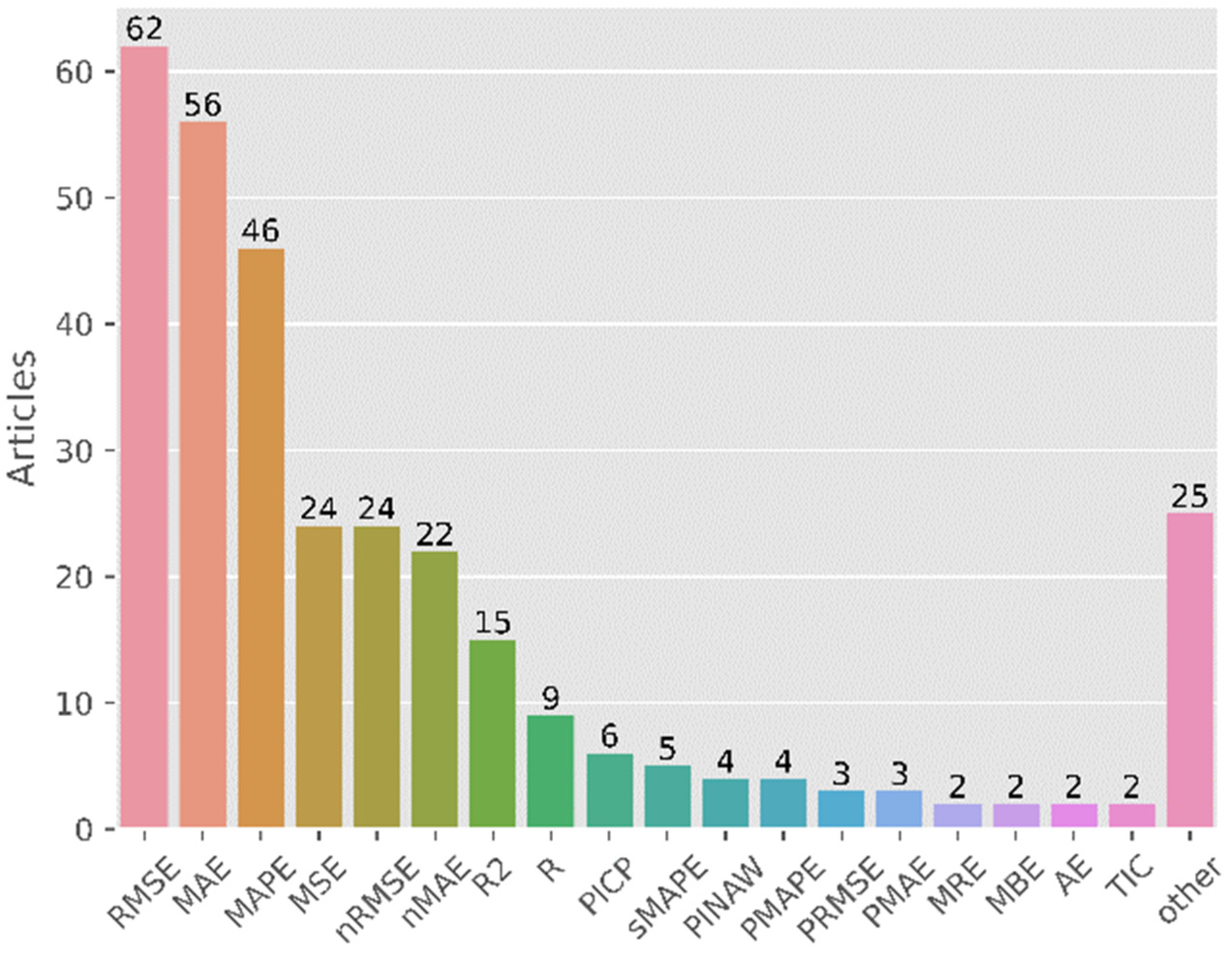
| Use | Metric | Number of Times Used |
|---|---|---|
| Frequent | RMSE, MAE, and MAPE | 46–62 |
| Occasional | MSE, nRMSE, nMAE, and R2 | 15–24 |
| Seldom | R, PICP, sMAPE, MBE, MRE, …, TIC | 2–9 |
| Rare | Other Metrics | 1 |
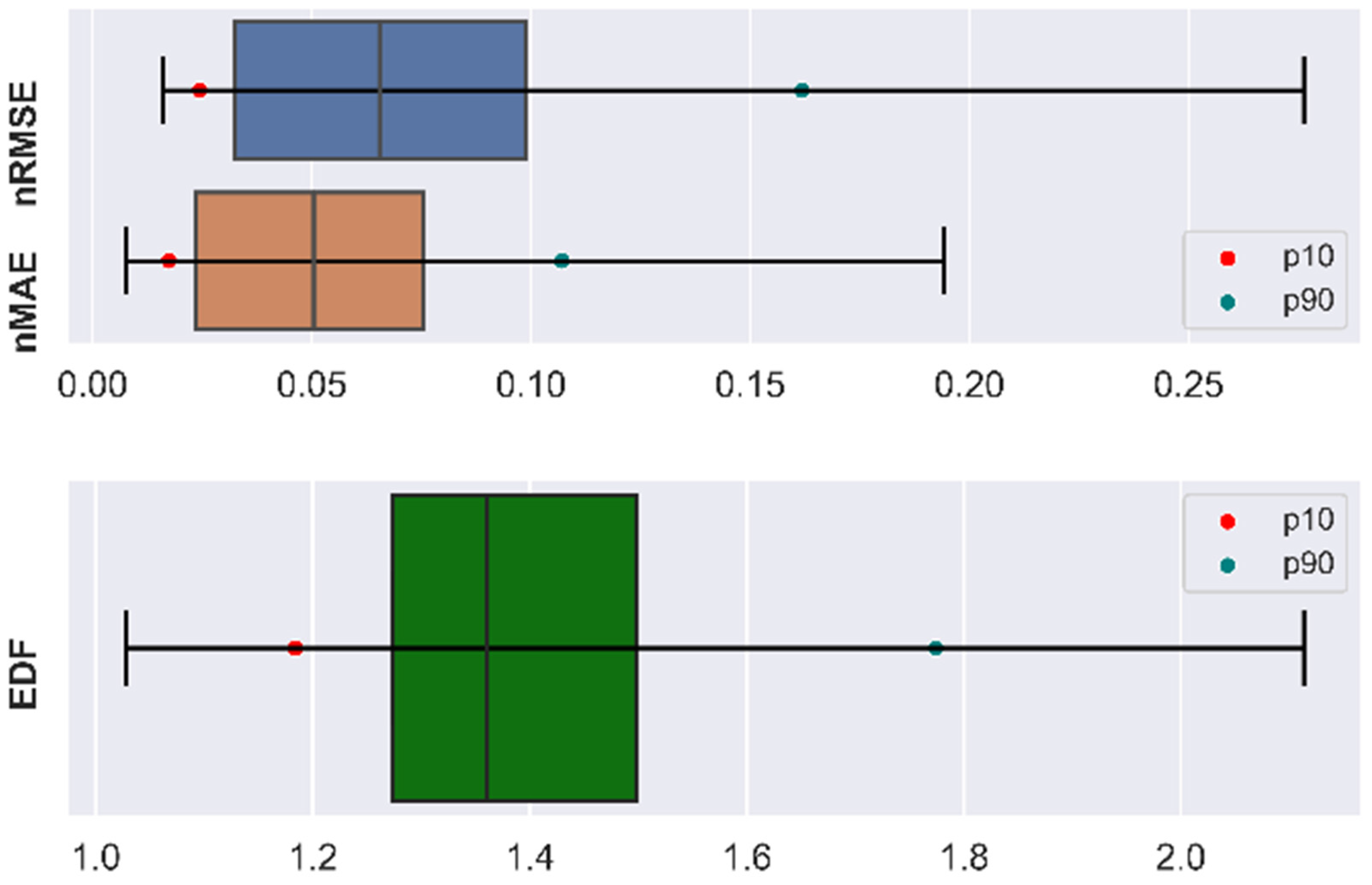
| Descriptive Statistics | nRMSE | nMAE | EDF |
|---|---|---|---|
| Mean | 0.0787 | 0.0566 | 1.4160 |
| Standard deviation | 0.0578 | 0.0407 | 0.2307 |
| Minimum | 0.0162 | 0.0077 | 1.0283 |
| Maximum | 0.2762 | 0.1942 | 2.1129 |
| Quotient of maximum/minimum | 17.05 | 25.22 | 1.75 |
| The 10th percentile | 0.0244 | 0.0174 | 1.1841 |
| The 25th percentile (lower quartile) | 0.0324 | 0.0236 | 1.2740 |
| The 50th percentile (median) | 0.0654 | 0.0504 | 1.3603 |
| The 75th (upper quartile) | 0.1007 | 0.0756 | 1.5019 |
| The 90 percentile | 0.1618 | 0.1070 | 1.7741 |
| Variance | 0.0033 | 0.0017 | 0.0562 |
| Skewness | 1.3448 | 1.2811 | 1.2939 |
| Kurtosis | 1.9858 | 1.8489 | 1.5423 |
Publisher’s Note: MDPI stays neutral with regard to jurisdictional claims in published maps and institutional affiliations. |
© 2022 by the authors. Licensee MDPI, Basel, Switzerland. This article is an open access article distributed under the terms and conditions of the Creative Commons Attribution (CC BY) license (https://creativecommons.org/licenses/by/4.0/).
Share and Cite
Piotrowski, P.; Rutyna, I.; Baczyński, D.; Kopyt, M. Evaluation Metrics for Wind Power Forecasts: A Comprehensive Review and Statistical Analysis of Errors. Energies 2022, 15, 9657. https://doi.org/10.3390/en15249657
Piotrowski P, Rutyna I, Baczyński D, Kopyt M. Evaluation Metrics for Wind Power Forecasts: A Comprehensive Review and Statistical Analysis of Errors. Energies. 2022; 15(24):9657. https://doi.org/10.3390/en15249657
Chicago/Turabian StylePiotrowski, Paweł, Inajara Rutyna, Dariusz Baczyński, and Marcin Kopyt. 2022. "Evaluation Metrics for Wind Power Forecasts: A Comprehensive Review and Statistical Analysis of Errors" Energies 15, no. 24: 9657. https://doi.org/10.3390/en15249657
APA StylePiotrowski, P., Rutyna, I., Baczyński, D., & Kopyt, M. (2022). Evaluation Metrics for Wind Power Forecasts: A Comprehensive Review and Statistical Analysis of Errors. Energies, 15(24), 9657. https://doi.org/10.3390/en15249657