Article

End-to-End Deep Neural Network Based Nonlinear Model Predictive Control: Experimental Implementation on Diesel Engine Emission Control

1
Department of Mechanical Engineering, University of Alberta, 116 St. and 85 Ave, Edmonton, AB T6G 2R3, Canada
2
Teaching and Research Area Mechatronics in Mobile Propulsion, RWTH Aachen University, Forckenbeckstrasse 4, 52074 Aachen, Germany
3
Institute of Automatic Control, RWTH Aachen University, Campus-Boulevard 30, 52074 Aachen, Germany
*
Author to whom correspondence should be addressed.
Energies 2022, 15(24), 9335; https://doi.org/10.3390/en15249335
Submission received: 8 November 2022 / Revised: 29 November 2022 / Accepted: 2 December 2022 / Published: 9 December 2022
(This article belongs to the Special Issue Experiments and Simulations of Combustion Process)

Abstract

:
In this paper, a deep neural network (DNN)-based nonlinear model predictive controller (NMPC) is demonstrated using real-time experimental implementation. First, the emissions and performance of a 4.5-liter 4-cylinder Cummins diesel engine are modeled using a DNN model with seven hidden layers and 24,148 learnable parameters created by stacking six Fully Connected layers with one long-short term memory (LSTM) layer. This model is then implemented as the plant model in an NMPC. For real-time implementation of the LSTM-NMPC, an open-source package acados with the quadratic programming solver HPIPM (High-Performance Interior-Point Method) is employed. This helps LSTM-NMPC run in real time with an average turnaround time of 62.3 milliseconds. For real-time controller prototyping, a dSPACE MicroAutoBox II rapid prototyping system is used. A Field-Programmable Gate Array is employed to calculate the in-cylinder pressure-based combustion metrics online in real time. The developed controller was tested for both step and smooth load reference changes, which showed accurate tracking performance while enforcing all input and output constraints. To assess the robustness of the controller to data outside the training region, the engine speed is varied from 1200 rpm to 1800 rpm. The experimental results illustrate accurate tracking and disturbance rejection for the out-of-training data region. At 5 bar indicated mean effective pressure and a speed of 1200 rpm, the comparison between the Cummins production controller and the proposed LSTM-NMPC showed a 7.9% fuel consumption reduction, while also decreasing both nitrogen oxides ( NO x ) and Particle Matter (PM) by up to 18.9% and 40.8%.

1. Introduction

Model-based optimal control techniques take advantage of significant improvements in system modeling, which has led to an increase in interest from various researchers in the past two decades. Some of these model-based control methods include the linear quadratic regulator [1,2], sliding mode controller [3,4,5], backstepping [6,7], adaptive control [8,9], and Model Predictive Control (MPC) [2,10,11,12,13]. Of these model-based controllers, MPC is an effective control strategy that is used widely in a range of applications from the chemical process industry to other industries such as automotive, power and energy systems, manufacturing, aerospace, healthcare, finance, and others [14]. All of these applications take advantage of the ability of MPC to provide an optimal control solution while allowing for the implementation of constraints on system states and controller outputs.
The models for the MPC controllers can be designed from various modeling methods including physics-based models (white box) and Machine Learning (ML) models based on experimental data (black box), as well as a mix of the physics and experimental data (gray box). Each of these models have their advantages and disadvantages. However, independent of the type of the model, one challenge with MPC is the controller sensitivity to model uncertainty and the required model computational time, especially for online optimization. Often, a trade-off exists, where improving model accuracy leads to increased model complexity, and these complex models exhibit nonlinear behavior requiring a more complicated control law such as Nonlinear MPC (NMPC) [15,16].
When compared with a feedforward neural network, A Recurrent Neural Network (RNN) is structurally similar with the addition of backward connections, which are needed for the sequential inputs [17]. With the use of parameter sharing, the RNN is highly computationally efficient. However, in RNNs, any long-term dependencies are difficult to capture in the model, as the prediction is only based on recent steps. This can also be described as the “vanishing gradient”, with the contribution of earlier steps becoming increasingly small. The challenge with RNN is the lack of long-term memory; however, memory cells can be introduced to help solve this problem. The most well-known form of these long-term memory cells is the Long Short-Term Memory (LSTM) cell [17].
Combining LSTM and NMPC, denoted as LSTM-NMPC, has shown its potential in optimal temperature set-point planning for energy efficient buildings [18], steam quality of thermal power units [19], and for motion prediction of surrounding vehicles in an autonomous vehicle [20]. With the success in these previous applications, LSTM-NMPC is now being considered for systems requiring fast time steps, such as control of an internal combustion engine. To implement this, embedded programming techniques are required, as discussed in this paper.
Specifically, the control of a diesel-fueled Compression Ignition (CI) engine is demonstrated in this work. The reliability and fuel conversion efficiency of CI engines has allowed these engines to be prevalent in a wide range of transportation sections. From the international transportation of goods in ships to use in public transportation systems including trains, buses, and medium-duty vehicles, the diesel engine is a common combustion system worldwide [21,22]. However, there are also disadvantages of diesel combustion, one of which is air pollution. With the need to move to a cleaner future, hybridization and electrification are getting increasing market share for light-duty passenger vehicles. However, challenges still remain for heavy-duty applications, which can be attributed to limited battery range, high battery costs, and increased total cost of ownership [21,22]. Because of this slow transition to electrification in the heavy-duty applications, there is an urgent need to provide emission reduction strategies that can be applied to the medium-duty and heavy-duty vehicles on the road today.
The challenge with applying LSTM-NMPC for cycle-to-cycle CI control is both the very short computational time available between engine cycles (e.g., 80 ms at engine speed of 1500 rpm) as well as the highly complex combustion process. The computational time restriction limits the complex models and high-fidelity models that can be included for real-time controller implementation. This competes with the need for detailed models that provide an accurate representation of the combustion process. Therefore, to enable the use of model-based controllers, significant work has been invested in the development of accurate and computationally efficient models [23,24,25,26,27]. However, the complexity of the CI combustion and the many various supporting systems in a CI engine has made physical-based model development time-consuming, and these models are often highly nonlinear and nonconvex. It is often necessary to utilize linearization or model-order reduction techniques of these complex models to allow for real-time control implementation [28].
The structure of most of the previous work in ML-based MPC for ICEs has been linear [10,12,29,30], or a nonlinear model that has been linearized [31,32,33]. Only a few previous researchers have explored a nonlinear data-driven structure [34,35,36]. Among these works, only one study was found that explores ML-based MPC control of a CI engine where a linearized model of a nonlinear ML-based model was used to design and implement a controller [31]. Furthermore, for considering real-time implementation, only linear models such as linear parameter varying (LPV) [12] or a linearized model [33] have been successfully implemented experimentally. Any previous ML-based Nonlinear MPC (NMPC) has only been implemented in simulation [34,35,36]. To the authors’ knowledge, this work shows the first time that a data-driven-based NMPC using Deep Neural Network (DNN) with a Long Short-Term Memory (LSTM) layer has been experimentally implemented that addresses the fast dynamics of ICEs. The advantages of the proposed LSTM-NMPC compared with prior physical-based NMPC studies [15] for CI engines include (i) less required development time to create high-fidelity engine combustion and emission models, (ii) less computational cost, (iii) no need for multilayer controller design (supervisory MPC and feedback NMPC), and (iv) including Maximum Pressure Rise Rate (MPRR) constraints.
Based on our previous simulation results [37,38,39], LSTM is a promising control method for ICE control, especially when compared with Support Vector Machine based LPV [38]. In our previous work, the reduction in NO x  emissions and fuel consumption using LSTM-NMPC [37] was implemented in simulation and validated using a processor-in-the-loop platform. This work extends our previous study [37] and is implemented on a real-time system using acados embedded programming. The previously developed controller is also further expanded to include Particle Matter (PM) emission reduction; thus, the  NO x  and PM trade-off can be optimized for the CI engine. In addition,  multi-pulse injection timing and duration, along with fuel pressure control, were added to gain more degrees of freedom to optimally control the CI engine-out emissions.
The main contributions of this paper are summarized as:
  • Developed a transient Indicated Mean Effective Pressure (IMEP), Maximum Pressure Rise Rate (MPRR), NO x  and PM concentration model using a DNN with one LSTM layer, which provides a high-accuracy model for nonlinear model predictive combustion engine control;
  • Real-time implementation of our previously proposed novel approach [37] to augment LSTM in NMPC (LSTM-NMPC) by augmenting LSTM hidden and cell states into a nonlinear optimization problem;
  • Design and real-time implementation of an NMPC using an ML model to minimize engine-out emission concentration, optimize NO x -PM trade off, and minimize fuel consumption, while maintaining the same output torque performance and illustrating significant improvements compared with the Cummins-calibrated production ECU.
The remainder of this paper is organized into four sections. Section 2 presents the development and design structure of the deep network model, as well as the experimental setup details. Section 3 provides details of the NMPC design and acados implementation. Experimental results, including comparison with the production ECU, are presented in Section 4. Finally, the main conclusions are summarized in Section 5.

2. Modeling

2.1. Deep Neural Network

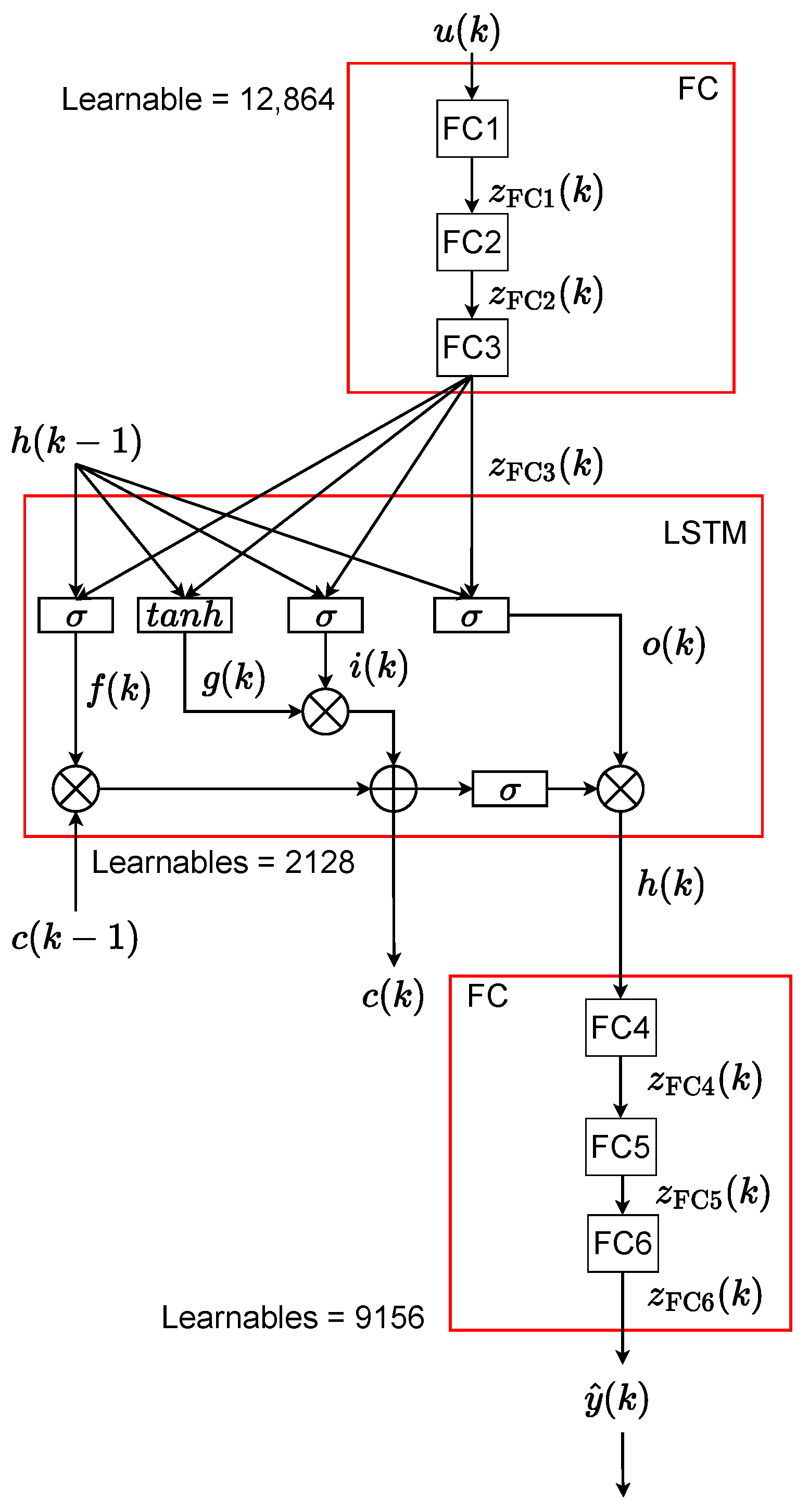
The Long Short-Term Memory (LSTM) cell is the most well-known form of RNN with long-term memory cells that are able to predict outputs while considering a long-term dependency. In comparison with basic RNNs, LSTMs employ a hidden state that is divided into two components: (i) the short-term state h ( k ) and (ii) the long-term state c ( k ) , as shown in Figure 1. The long-term state goes across the network and initially enters the forget gate and is multiplied by f ( k ) . Each time step adds new values (memories) to the input gate i ( k ) . As a result, some data are added and some are deleted at each time step [17].
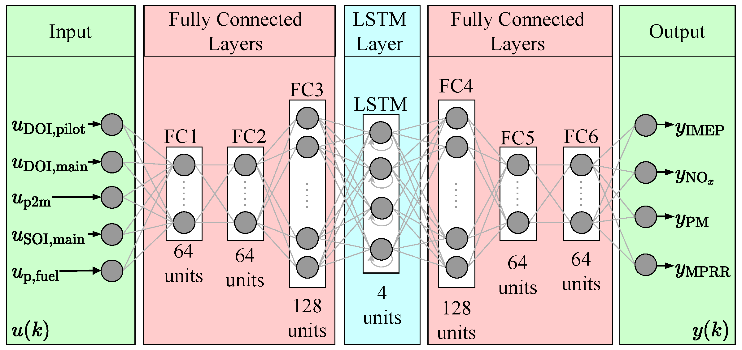
To model the CI engine emissions, a deep neural network with seven hidden layers, including 6 Fully Connected (FC) layers and one LSTM layer, is proposed, as shown in Figure 2. The input of this model is the start of injection (SOI) for the main injection ( u SOI , main ), duration of injection for both main ( u DOI , main ) and pilot injection ( u DOI , pilot ), duration between the end of pilot injection and the start of main injection pre-2-main time ( u p 2 m ), and fuel rail pressure ( u p , fuel ). The pre-2-main time is used instead of the SOI of pilot injection ( u SOI , pilot ) to allow for hardware constraints which limit the minimal time between injections to be implemented in the controller. This is necessary to prevent unintended overlapping injections where the injector has not fully closed. Figure 3 shows the relationship between SOI and DOI for both injections, as well as u p 2 m . The outputs of this model are nitrogen oxides ( y NO x ), Particle Matter ( y PM ), Maximum Pressure Rise Rate ( y MPRR ), and Indicated Mean Effective Pressure ( y IMEP ).
To capture the nonlinearity with the LSTM, more LSTM hidden units are needed, which result in a high number of hidden states and cell states. This resulted in a high computational cost for the MPC controller to find an optimal solution during real-time implementation. In our real-time implementation, doubling LSTM hidden units resulted in approximately doubling computational turnaround time from 63 ms to 130 ms, while this time must be within one engine cycle time (e.g., 80 ms at 1500 rpm) for cycle-by-cycle control. Instead of increasing LSTM hidden units, the Fully Connected (FC) layers are added before and after the LSTM layer to boost the network’s capacity for estimating the engine’s nonlinearity without significantly increasing the number of hidden and cell states.
To use this network inside a Nonlinear MPC (NMPC), a function using forward propagation is needed. To perform forward prorogation, first the LSTM and FC layers computations are evaluated. A computational graph (Figure 4) clarifies how the equations of the model are obtained. The LSTM computations are
i ( k ) = σ W u , i u ( k ) + W h , i h ( k 1 ) + b i
f ( k ) = σ W u , f u ( k ) + W h , f h ( k 1 ) + b f
g ( k ) = tanh W u , g u ( k ) + W h , g h ( k 1 ) + b g
o ( k ) = σ W u , o u ( k ) + W h , o T h ( k 1 ) + b o
c ( k ) = f ( k ) c ( k 1 ) + i ( k ) g ( k )
h ( k ) = o ( k ) tanh c ( k )
where W u , ( f , g , i , o ) are the weight matrices applied to the input vector u ( k ) and W h , ( f , g , i , o ) are the weight matrices of the previous short-term state  h ( k ) . In this equation, ⊙ is an element-wise multiplication and b ( f , g , i , o ) are the biases. In Equations (1a)–(1f), i ( k ) is the input gate, f ( k ) is the forget gate, g ( k ) is the cell candidate, o ( k ) is the output gate, c ( k ) is the cell state, and  h ( k ) is the hidden state. Two activation functions are used in Equations (1a)–(1f), which are given as: (i) tanh ( z ) activation function:
tanh ( z ) = e 2 z 1 e 2 z + 1
(ii) σ ( z ) activation function:
σ ( z ) = 1 1 + e z
An FC layer equation with Rectified Linear Unit (ReLU) activation function is defined as
z FC ( k ) = ReLU ( W FC T u ( k ) + b FC )
where ReLU activation function is defined as
ReLU = 0 if z 0 z if z > 0
The computational graph of this network is shown schematically in Figure 4. Based on this graph, and using Equations (1a)–(1f) and (4), the model equations are:
z FC 1 ( k ) = ReLU W FC 1 T u ( k ) + b FC 1
z FC 2 ( k ) = ReLU W FC 2 T z FC 1 ( k ) + b FC 2
z FC 3 ( k ) = ReLU W FC 3 T z FC 2 ( k ) + b FC 3
i ( k ) = σ W u , i z FC 3 ( k ) + W h , i h ( k 1 ) + b i
f ( k ) = σ W u , f z FC 3 ( k ) + W h , f h ( k 1 ) + b f
g ( k ) = tanh W u , g z FC 3 ( k ) + W h , g h ( k 1 ) + b g
o ( k ) = σ W u , o z FC 3 ( k ) + W h , o h ( k 1 ) + b o
c ( k ) = f ( k ) c ( k 1 ) + i ( k ) g ( k )
h ( k ) = o ( k ) tanh c ( k )
z FC 4 ( k ) = ReLU W FC 4 h ( k ) + b FC 4
z FC 5 ( k ) = ReLU W FC 5 z F C 4 ( k ) + b FC 5
y ( k ) = W FC 6 z FC 5 ( k ) + b FC 6
where W FC , i and b FC , i are the weights and biases of the fully connected layer where i { 1 , 2 , 3 , 4 , 5 , 6 } , W u , ( f , g , i , o ) are the weight matrices of the input vector u ( k ) , and W h , ( f , g , i , o ) are the weight matrices of the previous short-term states h ( k ) .
For training with experimental data, a standard cost function [17] of this network is defined as
J ( W , b ) = 1 m k = 1 m L y ^ ( k ) , y ( k ) + λ 2 m l = 1 L | | W [ l ] | | 2 2
where L y ^ ( k ) , y ( k ) is the loss function, m is the number of data points, y ^ ( k ) is measured output, and y ( k ) is predicted output. A Mean Squared Error (MSE) loss function is used, which is defined as
L y ^ ( k ) , y ( k ) = 1 m k = 1 m ( y ^ ( k ) y ( k ) ) 2
In Equation (9), λ is the regularization coefficients and | | W [ l ] | | 2 2 is the Euclidean norm, which is defined as
| | W [ l ] | | 2 2 = i = 1 n [ l ] j = 1 n [ l 1 ] ( w i j [ l ] ) 2

2.2. Training Model: Diesel Engine Modeling

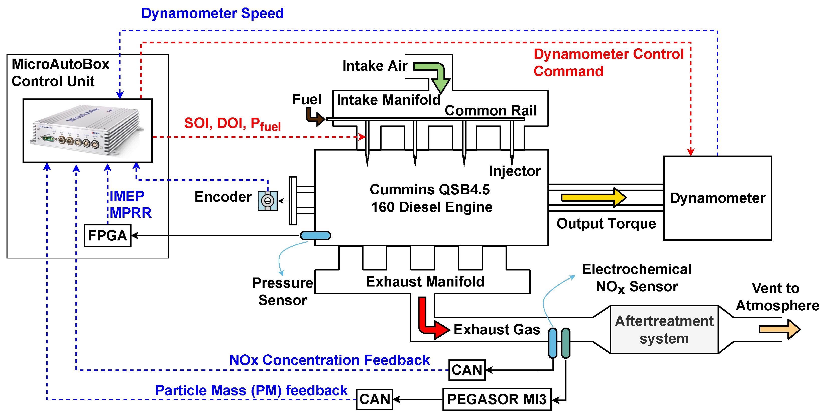
Experimental data were collected from a 4.5-liter medium-duty Cummins diesel engine to parameterize the model. The schematics of the experimental setup of the Cummins QSB4.5 160 diesel engine is shown in Figure 5 and Figure 6. NO x  emission concentration from the engine are measured using a Bosch sensor with ECM electronics (P/N: 06-05). A Pegasor Particle Sensor (PPS-M) is used to measure Particle Matter (PM). Additional details regarding the experimental setup can be found in [3,40,41,42].
The in-cylinder pressure is recorded using a National Instruments Data Acquisition Systems (DAQ) at a 0.1 resolution. This pressure signal is simultaneously provided to the Field Programmable Gate Array (FPGA) board contained in the prototyping ECU. More specifications of the MicroAutoBox II (MABX) prototyping ECU are provided in Table 1. The MABX II contains two main boards a CPU and FPGA. The CPU (ds1401) is used for replicating the production Cummins ECU tables, as well as for the implementation of the NMPC developed in this work.
The Xilinx Kintex-7 FPGA contained within the MABX is used to calculate various combustion metrics in real time. These include IMEP and MPRR, which are transferred from the FPGA to CPU for use as input to the NMPC. Details regarding the real-time calculation of IMEP and MPRR can be found in [27,43].
To develop this deep network, which has 24,148 learnable parameters, a large data set including 65,000 consecutive engine cycles is used. Therefore, the diesel engine was run for 65,000 cycles, and all five inputs, including the SOI of main ( u SOI , main ( k ) ), DOI of main ( u DOI , main ( k ) ), DOI of pilot ( u DOI , pilot ( k ) ), p2m time ( u p 2 m ( k ) ), and fuel rail pressure ( u p , fuel ( k ) ), are changed randomly using a pseudo-random binary sequence (PRBS). A random signal is used to change both the amplitude and frequency of these five inputs.
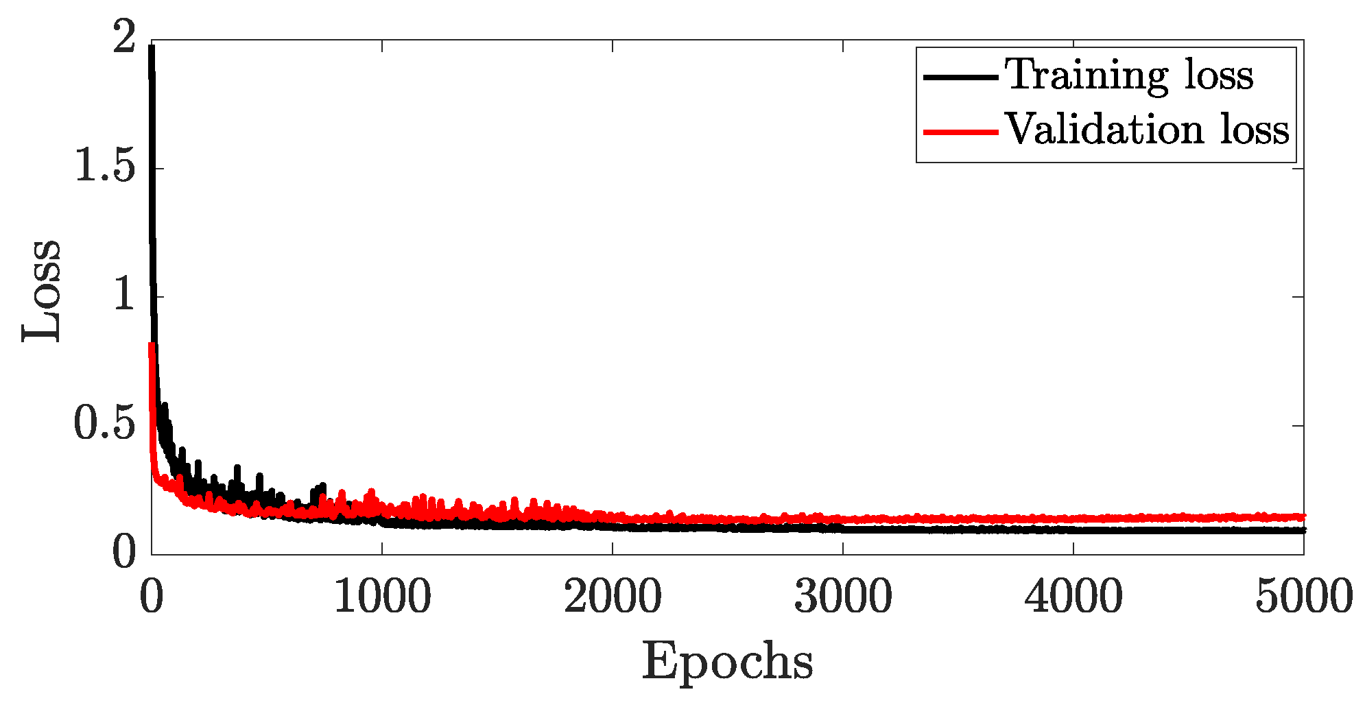
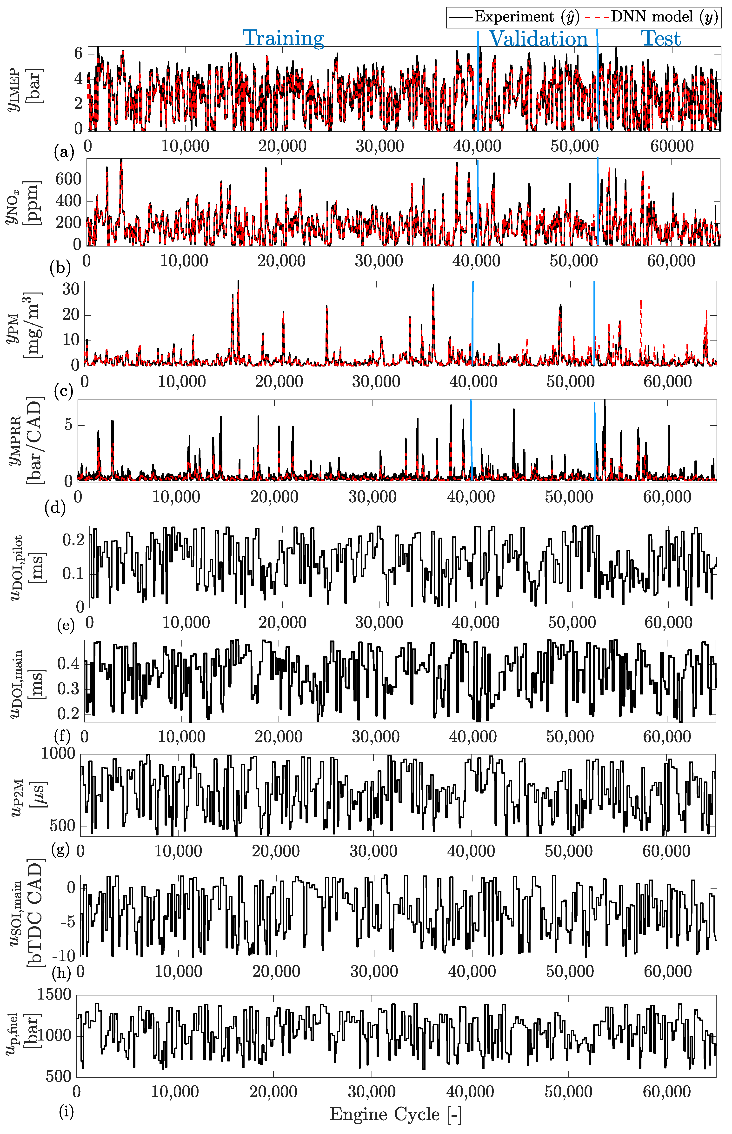
Table 2 summarizes the training information for the proposed network. To train this model, the Adam algorithm was used in the MATLAB Deep Learning Toolbox © . The loss function vs. iteration for the proposed deep network is given in Figure 7, where the loss functions converge to a minimal value. Additionally, the validation loss function converges to the training loss function, suggesting that neither overfitting nor underfitting has occurred [17].
The training and validation results of the proposed model are compared to the experimental values in Figure 8. Where cycles 1 to 40,000 are utilized for training, cycles 40,001 to 52,000 are used for validation, and cycles 52,001 to 65,000 are used for testing. In this figure, the SOI of pilot ( SOI pilot ) is calculated based on P2M time and illustrated to improve understanding of the controller behavior.
The accuracy of this model for each output is summarized in Table 3. For accuracy, the Root Mean Square Error (RMSE) and Normalized Root Mean Square Error (NRMSE) are used, which are defined as
RMSE = k = 0 N 1 ( y ^ ( k ) y ( k ) ) N
NRMSE = R M S E y m a x y m i n
As presented in Table 3, IMEP is the most difficult parameter for the model to predict, as shown by the 7% error in training, while other outputs are predicted with less than 3% error. The same trend can be seen for the testing data, where IMEP has a 10% error, while both emissions have errors of less than 8%. MPRR prediction is more accurate than others for test data, with a 2.7% error. The model can be further tuned to improve prediction accuracy by adding more hidden and cell states to the LSTM layer; however, by adding more states, it causes a significant increase in the computational time of the model on the real-time hardware. Therefore, this model has been improved only by adjusting the number of hidden units of the fully connected layers. This model is used for the NMPC design in the subsequent section.

3. Controller Design

3.1. Nonlinear Model Predictive Control

This section provides details on the design and implementation of the proposed Nonlinear Model Predictive Control (NMPC) algorithm. In NMPC, the current control input is computed by solving a nonlinear program at each sample instance. The underlying optimization problem consists of a model-based prediction of the system’s behavior, starting from the current state. The selected cost function minimizes engine-out emissions NO x  and PM concentrations, while simultaneously trying to reduce fuel consumption and maintaining the requested output torque. Additionally, the NMPC must meet constraints on the control output and engine combustion metrics. Finally, the developed NMPC is imported to the real-time experimental implementation on the dSPACE MABX II for diesel engine control.

3.2. Nonlinear State-Space Representation

The computation graph of the Deep Neural Network, derived in Section II, can be summarized into a sequence of fully connected layers at the input (Equations (6a)–(6c)), an LSTM layer (Equations (7a)–(7f)), and another sequence of fully connected layers at the output (Equations (8a)–(8c))
z FC 3 ( k ) = f FC , in u ( k )
c ( k ) h ( k ) = f LSTM c ( k 1 ) , h ( k 1 ) , z FC 3 ( k )
y ( k ) = f FC , out h ( k )
Eliminating the intermediate value z FC 3 ( k ) results in
c ( k ) h ( k ) = f c ( k 1 ) , h ( k 1 ) , u ( k )
y ( k ) = f FC , out h ( k )
If the hidden and cell states are now identified as an overall state vector x ( k ) = c ( k 1 ) , h ( k 1 ) , the resulting system of equations
x ( k + 1 ) = f x ( k ) , u ( k )
y ( k ) = f FC , out x ( k + 1 )
is almost represented by a standard nonlinear state-space representation of a dynamic system. In the standard formulation, however, the output depends only on the current state x ( k ) and input u ( k ) . One way to bring the LSTM-based network into the standard form is to adapt the definition of the engine cycle, accounting for the output after the control actions to the following cycle. Here, we simply substitute the next state in the output function by its definition, resulting in a nonlinear output function
x ( k + 1 ) = f x ( k ) , u ( k )
y ( k ) = f FC , out f x ( k ) , u ( k ) = g x ( k ) , u ( k )
with
x ( k ) = c ( k 1 ) h ( k 1 ) R 8 ,
y ( k ) = y IMEP ( k ) y NO x ( k ) y PM ( k ) y MPRR ( k ) R 4 ,
u ( k ) = u DOI , pilot ( k ) u DOI , main ( k ) u p 2 m ( k ) u SOI , main ( k ) u p , fuel R 5 .
Except for the duration of fuel injection, there are no desired setpoints for the other input variables. A positive definite weighting matrix for the control inputs would thus force an unnecessary compromise between tracking of the output and the manipulated variables. By introducing the change in manipulated variables as new inputs [44,45], the positive definite weighting matrix only drives the change to be zero, posing no conflict in reaching the desired output setpoints.
x ( k + 1 ) u ( k ) x ˜ ( k + 1 ) = f ( x ( k ) , u ( k 1 ) + Δ u ( k ) ) u ( k 1 ) + Δ u ( k ) f ˜ ( x ˜ ( k ) , Δ u ( k ) )
y ( k ) u ( k 1 ) y ˜ ( k ) = g ( x ( k ) ) u ( k 1 ) g ˜ ( x ˜ ( k ) ) .
Both the absolute inputs as well as their rate of change can be penalized in the cost function.

3.3. Optimal Control Problem

Given Equations (23a) and (23b), the discrete Optimal Control Problem (OCP) is defined as follows
Δ u 0 , , Δ u N x ˜ 0 , , x ˜ N y ˜ 0 , , y ˜ N i = 0 N r i y ˜ i Q 2 + Δ u i R 2 x ˜ 0 = x ( k ) , u ( k 1 ) x ˜ i + 1 = f ˜ ( x ˜ i , Δ u i ) i H \ N y ˜ i = g ˜ ( x ˜ i , Δ u i ) i H u min F u · y ˜ k u max i H y min F y · y ˜ k y max i H
where H = 0 , 1 , , N . The subscripts i indicate that the variables are part of the internal computations of the NMPC controller, whereas x ( k ) and u ( k 1 ) are the actual model’s current state and the previously applied control input, respectively. In this formulation, the nonlinear output function is stated as part of the constraints by introducing the augmented output as an optimization variable, allowing a linear least squares cost function. The reference r ˜ i and the weighting matrix Q are selected such that deviations from the requested load are penalized while minimizing NO x  and PM emission concentrations, as well as the amount of injected fuel
r ˜ i = r IMEP , i , 0 , 0 , 0 , 0 , 0 , 0 , 0 , 0 ,
Q = diag q IMEP , q NO x , q PM , 0 , r DOI , pilot , r DOI , main , 0 , 0 , 0 .
The specific cost function J thus reads as
(27) J = i = 0 N r IMEP , i y IMEP , i q IMEP 2 Load Tracking + (28) y NO x , i q NO x 2 + y PM , i q PM 2 Emission Reduction + (29) u DOI , pilot , i r DOI , pilot 2 + u DOI , main , i r DOI , main 2 Fuel consumption reduction + (30) Δ u i R 2
The weighting matrix R is a diagonal matrix with positive elements defined as
(31) R = diag ( r Δ u DOI , pilot , r Δ u DOI , pilot , r Δ u DOI , main , r Δ u SOI , main , (32)       r Δ u p 2 m , r Δ u p , fuel ) .
One advantage of NMPC is the ability to impose constraints on inputs and outputs. F u and F y are diagonal matrices with ones at the locations of bounded outputs and inputs.
The limits are imposed on IMEP to limit the engine to low–mid load operation. The upper IMEP constraint is below the engine maximum load but is imposed to keep the engine operating near the model calibration range for initial NMPC real-time implementation.
The upper limits for NO x and PM are used to constrain peak emission concentration levels and can be set to meet emission standards. The limits of 500 ppm for NO x and 10  mg / m 3 for PM were selected for this work based on the maximum engine-out emissions recorded when operating the engine using the production ECU.
Controlling the maximum pressure rise rate (MPRR) is crucial in combustion engines to ensure quiet and safe engine operation at various engine loads. MPRR is the rate at which the pressure increases in the cylinder, and the maximum permissible MPRR is engine- and application-dependent. Here, a typical 5 bar/CAD constraint is implemented to ensure no engine damage [10].
Constraints are also imposed on the DOI for both the pilot and main injections. The minimum DOI is limited to keep the injector within its calibration range. The upper limit is defined as 25% higher than the maximum observed injection with the production ECU.
The SOI main is constrained on both the upper and lower ends. Early SOI is restricted to avoid early combustion phasing, which can result in high engine noise and low thermal efficiency or engine damage at extreme values. Additionally, late SOI is limited to avoid low thermal efficiency and elevated exhaust gas temperatures. The p2m time is constrained for short durations based on hardware limitations to ensure the injector has fully closed before opening for the main injection. The upper limit is to restrict too early pilot injections. Finally, a limit for the fuel pressure is imposed to keep the commanded fuel pressure within the normal operating range of the injectors. Table 4 summarizes the implemented limitations on outputs and manipulated variables.

3.4. Implementation and Deployment to Real-Time Hardware

The development of control algorithm in real time on the dSPACE hardware through MATLAB/ Simulink is demonstrated in this section. Furthermore, the available computation time for the NMPC controller is dependent on the speed of the engine. At 1200 rpm, one engine cycle lasts 100 ms, while at 1800 rpm, only 66.7  ms are available. To meet the real-time requirements, a computationally efficient algorithm is needed to provide feedback from the engine cycle to the next cycle. For these reasons, the NMPC controller is implemented in MATLAB/ Simulink using the free and open source package acados [46], since simulation results in [37] indicate that it outperforms MATLAB’s MPC toolbox in terms of computation time, both with the fmincon and FORCES PRO [47,48] backend.
The plant model is passed to acados through the discrete dynamics interface, as no discretization is required. For computation of the Hessian in the underlying Sequential Quadratic Programming (SQP) algorithm, the Gauss–Newton approximation is used by selecting the non-exact Hessian option. The resulting Quadratic Problems (QPs) within the SQP algorithm are solved using the Interior Point (IP)-based QP solver hpipm, which is provided by the acados package. Compared with Active-Set-based QP solvers such as qpOASES, hpipm shows a higher computation time on average but avoids worst case peaks, which eventually determine the feasible turnaround time.
The OCP in Equation (24) leads to a band-diagonal structure in the matrices of the QPs within the SQP algorithm, which can be exploited by hpipm. Fully condensing the problem shows improvements in computation time in comparison with passing the sparse but high-dimensional problem formulation. The difference in runtime is attributed to the state vector having a higher dimension than the control input vector, and the engine dynamics only require small prediction horizons. The resulting OCP structure allows the fully condensed problem formulation to take full advantage of the condensation benefits [44,45].
Tuning of the weights, number of allowed SQP iterations, and the prediction horizon are performed by means of model in the loop simulations, where the NMPC controller runs against the controller internal model. Through these stimulative studies, the allowed number of SQP iterations is limited to five, while the prediction horizon is set to five.
After tuning, the algorithm is directly deployed to the embedded processor of the MABX II. The required cross-compiled libraries of acados can be obtained by following the “Embedded Workflow" in the acados documentation. On the embedded system, the NMPC shows a maximum turnaround time of 63.0  ms and an average of 62.3  ms, which is feasible for real-time implementation for the targeted engine speeds.
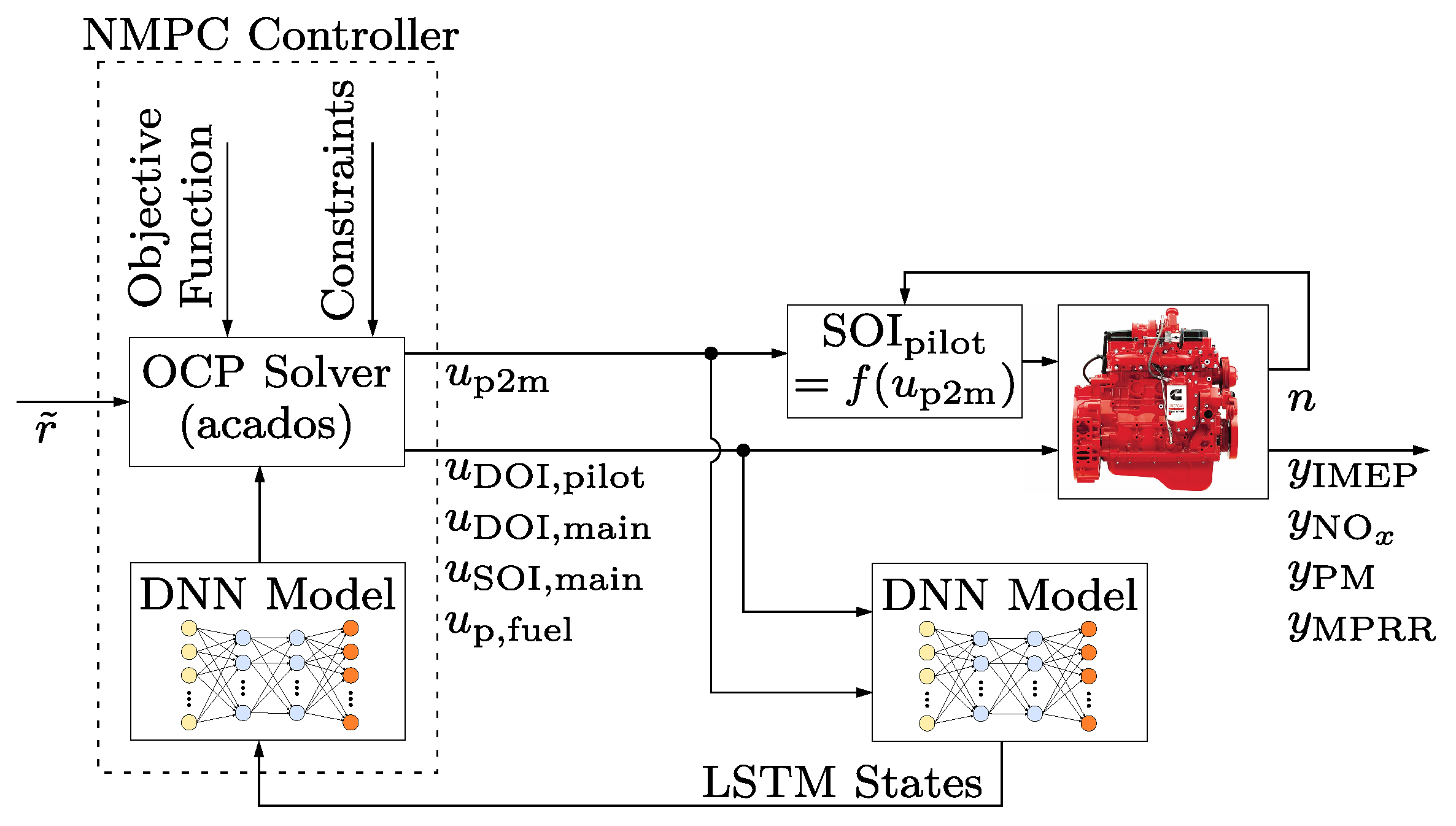
Figure 9 illustrates the setup of the experiments conducted on the testbed. The current cell and hidden states required by the controller are estimated by the derived DNN model that is running in parallel to the real engine.
In the next section, the real-time implementation results of the developed NMPC controller along with comparison with the production Cummin’s ECU are presented.

4. Experimental Results: Diesel Emission Control

The developed LSTM-NMPC is experimentally tested for IMEP tracking performance while minimizing emission concentration ( NO x  and PM) and fuel consumption, as well as meeting constraints on MPRR and SOI. The controller is subjected to step and smooth changes to create a bandwidth of approximately 1 Hz in target IMEP. Then, to test the controller’s robustness, it is evaluated by changing in engine speed while maintaining a constant IMEP. Finally, this controller is compared with the production ECU, which serves as a benchmark (BM) for comparison with the NMPC. To provide a BM, the Cummins production ECU is duplicated on the dSPACE MABX.

4.1. Experimental Results in Changing IMEP

The deep neural network based NMPC is first experimentally evaluated for its load tracking performance by following a step reference between 2 and 6 bar IMEP. This load range is selected to match the lower and upper bounds of the training data that are used for model development, as previously described. Figure 10 shows the multiple steps that are used to understand the performance of the controller on engine inputs and outputs.
The NMPC is capable of achieving the target IMEP within a cycle. There is a slight overshoot and some oscillations that can be seen after both the increase and decrease in target value. The oscillation in IMEP after the step change can be attributed to the relatively slow dynamics of the fuel pump and resulting oscillation in fuel pressure, as seen in Figure 10h. The delay in the fuel system to change pressure was not modeled, and the NMPC assumes instantaneous changes in pressure, which are not possible given the common rail fuel system used. However, overall, the controller is capable of achieving the reference setpoint with a 0.26 bar average error and RMSE of 0.61 bar.
The changing NO x  and PM concentration can be seen in Figure 10b and Figure 10c, respectively. As expected, an increase in IMEP results in an increase in emissions. However, to better compare the improvement of the developed controller, it is compared with the production ECU (BM) later in this section.
The engine speed is controlled by dynamometer, and a variation of ±50 RPM is observed. Finally, it can be noted that there are no constraint violations in MPRR, DOI, SOI, fuel pressure, or other outputs.
The NMPC is then tested by providing a smooth IMEP setpoint with a bandwidth of approximately 1 Hz. The controller performance can be seen in Figure 11, where the NMPC is again able to successfully track the target load. Here, the controller is able to track the reference with a 0.16 bar average error and a RMSE of 0.20 bar. Again, the NMPC does not violate any of the constraints on inputs or outputs. As shown is Figure 11h, there is oscillation in the fuel rail pressure. The current IMEP tracking is acceptable; however, to further improve the controller, a more accurate fuel pressure controller may be required.
Overall, the developed NMPC performs very well at 1500 rpm, with an average of 0.21 bar tracking error (the deep neural network model is trained at this speed) for tracking both step and smooth IMEP setpoints with a bandwidth of approximately 1 Hz. Next, the robustness of the NMPC to a changing engine speed is experimentally tested. The model was developed at a constant speed, so a variation in engine speed is an unmodeled disturbance.

4.2. Experimental Results in Changing Engine Speed

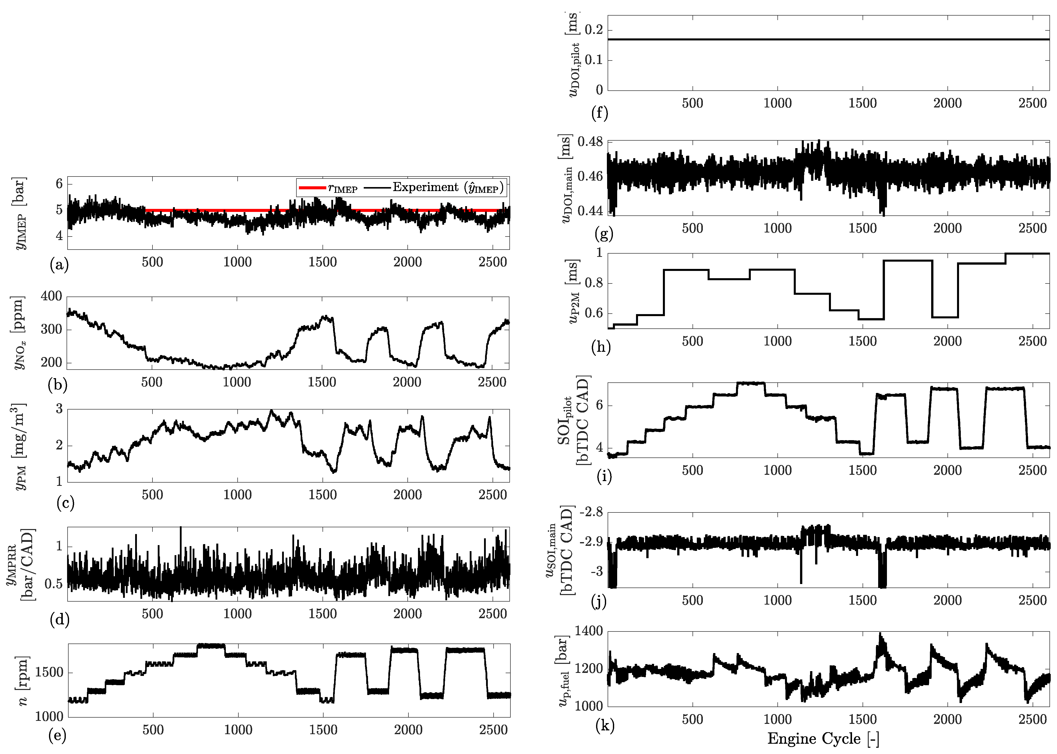
To further evaluate the developed NMPC, the engine speed is changed from 1200 to 1800 rpm at a constant IMEP of 5 bar. This test evaluates the model outside the range where it was identified (trained), as it was only trained at 1500 rpm. The controllers’ performance in tracking step changes in load is shown in Figure 12. Here, steps of 100 rpm are implemented for the first 1500 engine cycles, and then for the remaining cycles, larger steps of up to 500 rpm are tested. Overall, the controller is able to maintain the IMEP setpoint over changing speeds with an average error of 0.27 bar. Once again, the NMPC is able to maintain all constraints over the range of speeds tested.
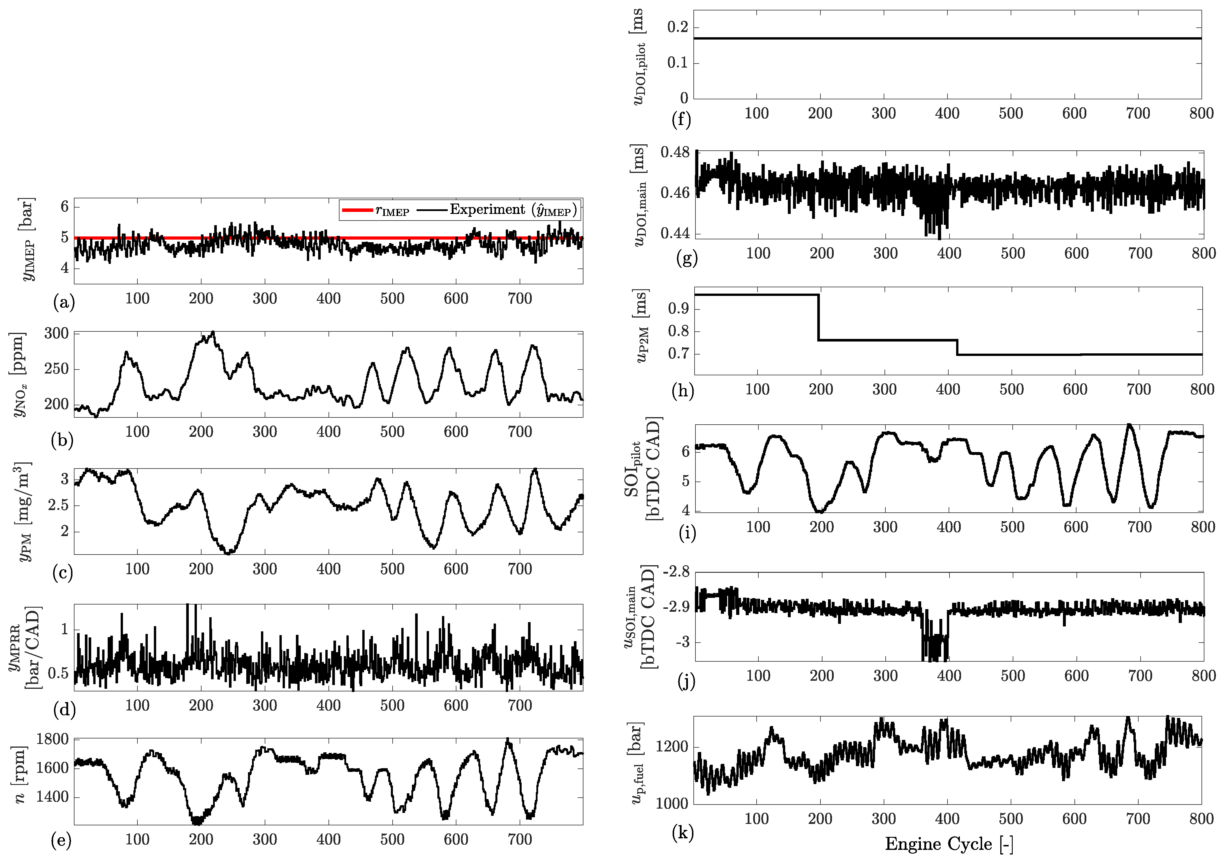
A similar result can be seen with smooth speed change with a bandwidth of approximately 1 Hz, as shown in Figure 13. Again, all constraints are maintained. The NMPC is able to maintain commanded engine load over step and smooth speed change with a bandwidth of approximately 1 Hz on the engine.

4.3. LSTM-NMPC vs. Cummins-Calibrated ECU

Now, the developed LSTM-NMPC controller is compared with the benchmark (BM) engine controller. In this work, the BM is taken as the replicated Cummins production ECU. Table 5 presents nine different load/speed cases varying between 2–6 bar IMEP and 1200–1800 rpm. Each table row represents an average of 200 cycles. It should be noted that the average IMEP may not necessarily perfectly match the reference value for either the BM or NMPC. Generally, the NMPC achieves closer to the reference value, since it uses measured IMEP (calculated from an in-cylinder pressure sensor with FPGA) as input to the NMPC controller, but the BM utilizes a feedforward table. However, for comparison, load-normalized emissions are used for both NO x  and PM, which are converted to g/kWh, which represents the mass of emission produced per generated energy. Similarly, thermal efficiencies of all controllers are compared.
Table 5 presents the average NO x , Particulate Matter (PM), Fuel Quantity (FQ), and thermal efficiency at the given operating point. Here, the percent difference of the NMPC compared with the BM is shown, where a negative value represents that the NMPC is below the BM. In all the cases tested, the NMPC is able to reduce the fuel consumption by 9.5%, while also increasing the thermal efficiency by an average of 2.5%.
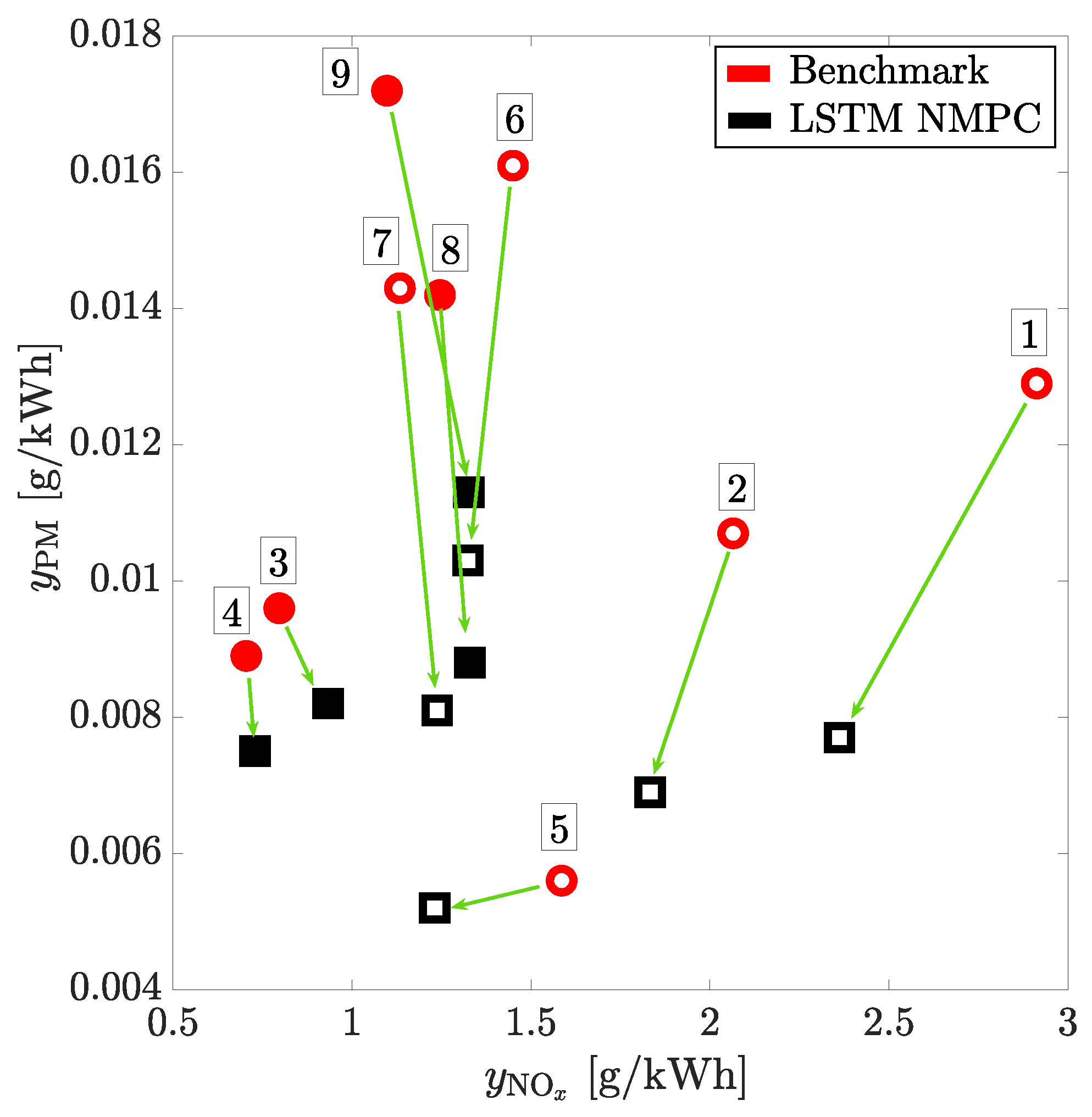
For the PM emissions, there is a significant reduction in emissions at every operating point. However, when looking at NO x  ,there is not a clear trend. At some operating points, there is an increase in NO x  emissions, while at others there is a decrease. Overall, on average, there is a slight decrease of 0.5% in NO x  emissions. However, a better comparison of the emission reduction can be seen in Figure 14, where the well-known trade-off between NO x  and PM is evaluated. Here, the importance of the cost function in the NMPC can be seen as the reduction in both NO x  and PM emissions from the upper end of their range. So, when significant PM is present, the NMPC focuses more on reducing PM and may allow a slight increase in NO x  if the value is fairly low, especially for cases 3 and 4. However, if both PM and NO x  are high, such as in cases 1 or 2, the NMPC reduces both. This is a significant advantage, as it shows that the NMPC is able to reduce both emissions when they are high and close to the upper boundary. Additionally, if one emission is comparable to the regulation boundary such as in case 9 for PM, it reduces it significantly by slightly increasing the NO x  value, which is lower than the regulated values for this engine. In this case, the well-known optimum PM and NO x  trade-off can be handled by NMPC.

5. Conclusions

This work demonstrated that deep learning and Nonlinear Model Predictive Control (NMPC) can be successfully implemented in real time for the minimization of compression ignition engine-out emissions and fuel consumption, while imposing constraints on engine inputs and outputs. The emissions and performance characteristics of a 4.5-liter 4-cylinder Cummins compression ignition engine were modeled using a deep network with seven hidden layers and 24,148 learnable parameters constructed by stacking fully connected layers with a Long Short-Term Memory (LSTM) layer. This model was then used to design and implement an NMPC in real-time.
To develop this LSTM-NMPC, the open-source software acados was used in combination with the quadratic programming solution HPIPM (High-Performance Interior-Point Method). This acados embedded programming approach enables real-time operation of the LSTM-NMPC with an average turnaround time of 62.3 milliseconds on a dSPACE MicroAutoBoxII. To implement the controller, the FPGA for online calculation of IMEP and MPRR cycle by cycle, fast PM, and NO x  sensors were needed.
When compared with the Cummins-calibrated production controller, the proposed LSTM-NMPC saved fuel by 7.3–14.9 percent, while boosting thermal efficiency by 0.1–4.7 percent depending on the engine operating point. This controller was capable of reducing nitrogen oxides ( NO x ) and Particle Matter (PM) concentrations by up to 22.4 and 43.6 percent, respectively. The well-known trade-off between NO x and particulate emissions was analyzed, where the controller showed that when large PM is present, the NMPC prioritizes PM reduction while allowing a slight rise in NO x if the amount is relatively low. However, if both PM and NO x levels are high, the NMPC effectively reduces both. This is a significant benefit, since it demonstrates the NMPC’s ability to reduce emissions when they are near the imposed constraints or regulatory limits.
To determine the controller’s robustness for operation outside the training range of the model, the controller was evaluated at speeds ranging from 1200 to 1800 rpm. The experimental findings confirm that tracking and disturbance rejection capability of the designed controller. The controller was able to maintain the IMEP setpoint with an average error of 0.16 and 0.27 bar for step and smooth speed change. No constraint violation was observed in all cases tested for state, output, and input constraints.

Author Contributions

Conceptualization, D.C.G., A.N. and A.W.; methodology, E.N. and A.N.; software, D.C.G., A.N., A.W. and J.M.; formal analysis, D.C.G. and A.N.; resources, D.A., M.S., J.A. and C.R.K.; writing—original draft preparation, D.C.G. and A.N.; writing—review and editing, all authors; visualization, D.C.G. and A.N.; supervision, D.A., M.S., J.A. and C.R.K.; project administration, J.A. and C.R.K.; funding acquisition, J.A. and C.R.K. All authors have read and agreed to the published version of the manuscript.

Funding

The research was performed under the Natural Sciences Research Council of Canada Grant 2016-04646 and as part of the Research Group (Forschungsgruppe) FOR 2401 “Optimization based Multiscale Control for Low Temperature Combustion Engines,” which is funded by the German Research Association (Deutsche Forschungsgemeinschaft, DFG). The research is also partially funded by Future Energy Systems and Alberta innovates at the University of Alberta.

Data Availability Statement

Not applicable.

Conflicts of Interest

The authors declare no conflict of interest. The funders had no role in the design of the study; in the collection, analyses, or interpretation of data; in the writing of the manuscript, or in the decision to publish the results.

References

  1. López, J.D.; Espinosa, J.J.; Agudelo, J.R. LQR control for speed and torque of internal combustion engines. IFAC Proc. Vol. 2011, 44, 2230–2235. [Google Scholar] [CrossRef] [Green Version]
  2. Bemporad, A.; Morari, M.; Dua, V.; Pistikopoulos, E.N. The explicit linear quadratic regulator for constrained systems. Automatica 2002, 38, 3–20. [Google Scholar] [CrossRef]
  3. Norouzi, A.; Ebrahimi, K.; Koch, C.R. Integral discrete-time sliding mode control of homogeneous charge compression ignition (HCCI) engine load and combustion timing. IFAC-PapersOnLine 2019, 52, 153–158. [Google Scholar] [CrossRef]
  4. Norouzi, A.; Adibi-Asl, H.; Kazemi, R.; Hafshejani, P.F. Adaptive sliding mode control of a four-wheel-steering autonomous vehicle with uncertainty using parallel orientation and position control. Int. J. Heavy Veh. Syst. 2020, 27, 499–518. [Google Scholar] [CrossRef]
  5. Altintas, Y.; Erkorkmaz, K.; Zhu, W.H. Sliding mode controller design for high speed feed drives. CIRP Ann. 2000, 49, 265–270. [Google Scholar] [CrossRef]
  6. Norouzi, A.; Masoumi, M.; Barari, A.; Sani, S.F. Lateral control of an autonomous vehicle using integrated backstepping and sliding mode controller. Proc. Inst. Mech. Eng. Part K J. Multi-Body Dyn. 2019, 233, 141–151. [Google Scholar] [CrossRef]
  7. Madani, T.; Benallegue, A. Backstepping control for a quadrotor helicopter. In Proceedings of the 2006 IEEE/RSJ International Conference on Intelligent Robots and Systems, Beijing, China, 9–15 October 2006; pp. 3255–3260. [Google Scholar]
  8. Souder, J.S.; Hedrick, J.K. Adaptive sliding mode control of air–fuel ratio in internal combustion engines. Int. J. Robust Nonlinear Control. IFAC-Affil. J. 2004, 14, 525–541. [Google Scholar] [CrossRef]
  9. Lavretsky, E.; Wise, K.A. Robust adaptive control. In Robust and Adaptive Control; Springer: London, UK, 2013; pp. 317–353. [Google Scholar]
  10. Basina, L.A.; Irdmousa, B.K.; Velni, J.M.; Borhan, H.; Naber, J.D.; Shahbakhti, M. Data-driven modeling and predictive control of maximum pressure rise rate in RCCI engines. In Proceedings of the IEEE Conference on Control Technology and Applications (CCTA 2020), Montreal, QC, Canada, 24–26 August 2020; pp. 94–99. [Google Scholar] [CrossRef]
  11. Cairano, S.D.; Bernardini, D.; Bemporad, A.; Kolmanovsky, I.V. Stochastic MPC With Learning for Driver-Predictive Vehicle Control and its Application to HEV Energy Management. IEEE Trans. Control Syst. Technol. 2014, 22, 1018–1031. [Google Scholar] [CrossRef]
  12. Irdmousa, B.K.; Rizvi, S.Z.; Velni, J.M.; Naber, J.; Shahbakhti, M. Data-driven modeling and predictive control of combustion phasing for RCCI Engines. In Proceedings of the American Control Conference (ACC 2019), Philadelphia, PA, USA, 10–12 July 2019; pp. 1–6. [Google Scholar] [CrossRef]
  13. Bemporad, A.; Borrelli, F.; Morari, M. Piecewise linear optimal controllers for hybrid systems. In Proceedings of the American Control Conference (ACC 2000), Chicago, IL, USA, 28–30 June 2000; Volume 2, pp. 1190–1194. [Google Scholar] [CrossRef]
  14. Lee, J.H. Model predictive control: Review of the three decades of development. Int. J. Control. Autom. Syst. 2011, 9, 415. [Google Scholar] [CrossRef]
  15. Liao-McPherson, D.; Huang, M.; Kim, S.; Shimada, M.; Butts, K.; Kolmanovsky, I. Model predictive emissions control of a diesel engine airpath: Design and experimental evaluation. Int. J. Robust Nonlinear Control 2020, 30, 7446–7477. [Google Scholar] [CrossRef]
  16. Di Cairano, S.; Doering, J.; Kolmanovsky, I.V.; Hrovat, D. Model Predictive Control of Engine Speed During Vehicle Deceleration. IEEE Trans. Control Syst. Technol. 2014, 22, 2205–2217. [Google Scholar] [CrossRef]
  17. Géron, A. Hands-On Machine Learning with Scikit-Learn, Keras, and TensorFlow: Concepts, Tools, and Techniques to Build Intelligent Systems; O’Reilly Media: Sebastopol, CA, USA, 2019. [Google Scholar]
  18. Jeon, B.K.; Kim, E.J. LSTM-Based Model Predictive Control for Optimal Temperature Set-Point Planning. Sustainability 2021, 13, 894. [Google Scholar] [CrossRef]
  19. Wang, Q.; Pan, L.; Lee, K.Y. Improving Superheated Steam Temperature Control Using United Long Short Term Memory and MPC. IFAC-PapersOnLine 2020, 53, 13345–13350. [Google Scholar] [CrossRef]
  20. Tang, X.; Zhong, G.; Yang, K.; Wu, J.; Wei, Z. Motion Planning Framework for Autonomous Vehicle with LSTM-based Predictive Model. In Proceedings of the 2021 5th CAA International Conference on Vehicular Control and Intelligence (CVCI), Tianjin, China, 29–31 October 2021; pp. 1–5. [Google Scholar] [CrossRef]
  21. Norouzi, A.; Heidarifar, H.; Shahbakhti, M.; Koch, C.R.; Borhan, H. Model Predictive Control of Internal Combustion Engines: A Review and Future Directions. Energies 2021, 14, 6251. [Google Scholar] [CrossRef]
  22. Aliramezani, M.; Koch, C.R.; Shahbakhti, M. Modeling, diagnostics, optimization, and control of internal combustion engines via modern machine learning techniques: A review and future directions. Prog. Energy Combust. Sci. 2022, 88, 100967. [Google Scholar] [CrossRef]
  23. Nair, V.; Sujith, R. A reduced-order model for the onset of combustion instability: Physical mechanisms for intermittency and precursors. Proc. Combust. Inst. 2015, 35, 3193–3200. [Google Scholar] [CrossRef]
  24. Ra, Y.; Reitz, R.D. A combustion model for multi-component fuels using a physical surrogate group chemistry representation (PSGCR). Combust. Flame 2015, 162, 3456–3481. [Google Scholar] [CrossRef]
  25. Oran, E.S.; Boris, J.P. Detailed modelling of combustion systems. Prog. Energy Combust. Sci. 1981, 7, 1–72. [Google Scholar] [CrossRef]
  26. Gordon, D.; Wouters, C.; Wick, M.; Lehrheuer, B.; Andert, J.; Koch, C.R.; Pischinger, S. Development and experimental validation of a field programmable gate array–based in-cycle direct water injection control strategy for homogeneous charge compression ignition combustion stability. Int. J. Engine Res. 2019, 20, 1101–1113. [Google Scholar] [CrossRef]
  27. Gordon, D.; Wouters, C.; Wick, M.; Xia, F.; Lehrheuer, B.; Andert, J.; Koch, C.R.; Pischinger, S. Development and experimental validation of a real-time capable field programmable gate array–based gas exchange model for negative valve overlap. Int. J. Engine Res. 2020, 21, 421–436. [Google Scholar] [CrossRef]
  28. Shahpouri, S.; Norouzi, A.; Hayduk, C.; Rezaei, R.; Shahbakhti, M.; Koch, C.R. Soot emission modeling of a compression ignition engine using machine learning. IFAC-PapersOnLine 2021, 54, 826–833. [Google Scholar] [CrossRef]
  29. Bao, Y.; Mohammadpour Velni, J.; Shahbakhti, M. An Online Transfer Learning Approach for Identification and Predictive Control Design With Application to RCCI Engines. In Proceedings of the Dynamic Systems and Control Conference, Virtual, 5–7 October 2020; Volume 84270. [Google Scholar] [CrossRef]
  30. Khoshbakht Irdmousa, B.; Naber, J.; Mohammadpour Velni, J.; Borhan, H.; Shahbakhti, M. Input-output Data-driven Modeling and MIMO Predictive Control of an RCCI Engine Combustion. IFAC-PapersOnLine 2021, 54, 406–411. [Google Scholar] [CrossRef]
  31. Ira, A.S.; Shames, I.; Manzie, C.; Chin, R.; Nešić, D.; Nakada, H.; Sano, T. A Machine Learning Approach for Tuning Model Predictive Controllers. In Proceedings of the 15th International Conference on Control, Automation, Robotics and Vision (ICARCV 2018), Singapore, 18–21 November 2018; pp. 2003–2008. [Google Scholar] [CrossRef]
  32. Lennox, B.; Montaguet, G.A.; Frith, A.M.; Beaumont, A.J. Non-linear model-based predictive control of gasoline engine air-fuel ratio. Trans. Inst. Meas. Control 1998, 20, 103–112. [Google Scholar] [CrossRef]
  33. Janakiraman, V.M.; Nguyen, X.; Assanis, D. An ELM based predictive control method for HCCI engines. Eng. Appl. Artif. Intell. 2016, 48, 106–118. [Google Scholar] [CrossRef]
  34. Wang, S.; Yu, D.; Gomm, J.; Page, G.; Douglas, S. Adaptive neural network model based predictive control for air–fuel ratio of SI engines. Eng. Appl. Artif. Intell. 2006, 19, 189–200. [Google Scholar] [CrossRef]
  35. Hu, Y.; Chen, H.; Wang, P.; Chen, H.; Ren, L. Nonlinear model predictive controller design based on learning model for turbocharged gasoline engine of passenger vehicle. Mech. Syst. Signal Process. 2018, 109, 74–88. [Google Scholar] [CrossRef]
  36. Batool, S.; Naber, J.; Shahbakhti, M. Data-Driven Modeling and Control of Cyclic Variability of an Engine Operating in Low Temperature Combustion Modes. IFAC-PapersOnLine 2021, 54, 834–839. [Google Scholar] [CrossRef]
  37. Norouzi, A.; Shahpouri, S.; Gordon, D.; Winkler, A.; Nuss, E.; Andert, J.; Shahbakhti, M.; Koch, C.R. Integration of Deep Learning and Nonlinear Model Predictive Control in Emission reduction of Compression Ignition Combustion Engines: A Simulative Study. arXiv Preprint 2022, arXiv:2204.00139. [Google Scholar] [CrossRef]
  38. Norouzi, A.; Shahpouri, S.; Gordon, D.; Winkler, A.; Nuss, E.; Abel, D.; Andert, J.; Shahbakhti, M.; Koch, C.R. Machine Learning Integrated with Model Predictive Control for Imitative Optimal Control of Compression Ignition Engines. arXiv Preprint 2022, arXiv:2204.00142. [Google Scholar] [CrossRef]
  39. Norouzi, A. Machine Learning and Deep Learning for Modeling and Control of Internal Combustion Engines. Ph.D. Thesis, University of Alberta, Edmonton, AB, Canada, 2022. [Google Scholar]
  40. Norouzi, A.; Gordon, D.; Aliramezani, M.; Koch, C.R. Machine Learning-based Diesel Engine-Out NOx Reduction Using a plug-in PD-type Iterative Learning Control. In Proceedings of the 2020 IEEE Conference on Control Technology and Applications (CCTA), Montreal, QC, Canada, 24–26 August 2020; pp. 450–455. [Google Scholar] [CrossRef]
  41. Aliramezani, M.; Norouzi, A.; Koch, C.R. Support vector machine for a diesel engine performance and NOx emission control-oriented model. IFAC-PapersOnLine 2020, 53, 13976–13981. [Google Scholar] [CrossRef]
  42. Norouzi, A.; Aliramezani, M.; Koch, C.R. A correlation-based model order reduction approach for a diesel engine NOx and brake mean effective pressure dynamic model using machine learning. Int. J. Engine Res. 2021, 22, 2654–2672. [Google Scholar] [CrossRef]
  43. Pfluger, J.; Andert, J.; Ross, H.; Mertens, F. Rapid Control Prototyping for Cylinder Pressure Indication. MTZ Worldw. 2012, 73, 38–42. [Google Scholar] [CrossRef]
  44. Diehl, M.; Ferreau, H.J.; Haverbeke, N. Efficient Numerical Methods for Nonlinear MPC and Moving Horizon Estimation. In Nonlinear Model Predictive Control: Towards New Challenging Applications; Magni, L., Raimondo, D.M., Allgöwer, F., Eds.; Springer: Berlin/Heidelberg, Germany, 2009; pp. 391–417. [Google Scholar] [CrossRef]
  45. Frison, G.; Kouzoupis, D.; Jørgensen, J.; Diehl, M. An efficient implementation of partial condensing for Nonlinear Model Predictive Control. In Proceedings of the 2016 IEEE 55th Conference on Decision and Control (CDC), Las Vegas, NV, USA, 12–14 December 2016; pp. 4457–4462. [Google Scholar] [CrossRef]
  46. Verschueren, R.; Frison, G.; Kouzoupis, D.; Frey, J.; van Duijkeren, N.; Zanelli, A.; Novoselnik, B.; Albin, T.; Quirynen, R.; Diehl, M. acados: A modular open-source framework for fast embedded optimal control. arXiv Preprint 2019, arXiv:1910.13753. [Google Scholar] [CrossRef]
  47. Domahidi, A.; Jerez, J. FORCES Professional. Embotech AG. 2014–2019. Available online: https://embotech.com/FORCES-Pro (accessed on 22 January 2021).
  48. Zanelli, A.; Domahidi, A.; Jerez, J.; Morari, M. FORCES NLP: An efficient implementation of interior-point methods for multistage nonlinear nonconvex programs. Int. J. Control. 2020, 93, 13–29. [Google Scholar] [CrossRef]
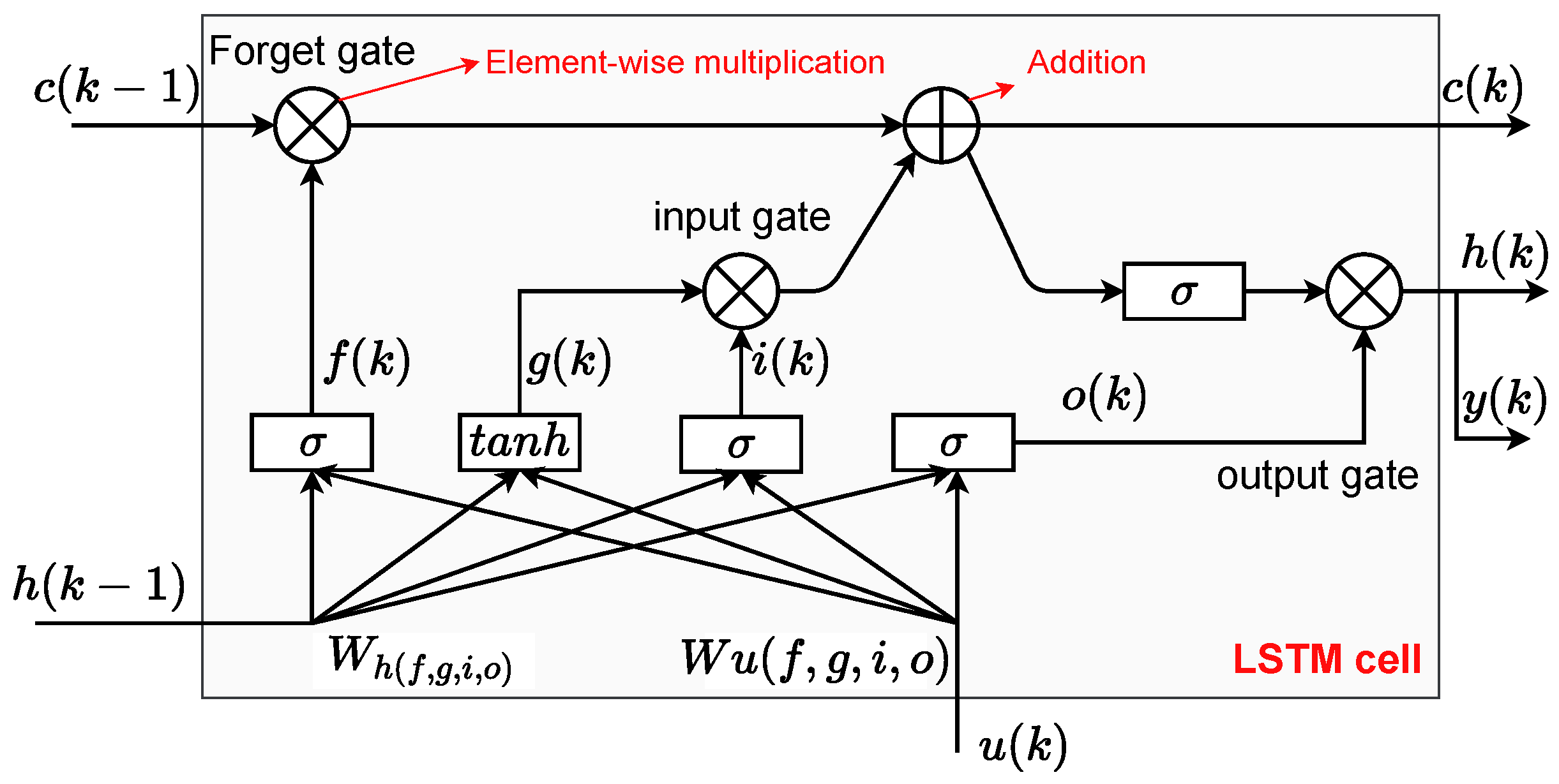
Figure 1. Long Short-Term Memory (LSTM) cell structure schematics.
Energies 15 09335 g001
Figure 2. Structure of the proposed deep neural network model for engine performance and emission concentration modeling. LSTM: Long Short-Term memory, SOI: start of injection, DOI: duration of injection, p, fuel: fuel rail pressure, IMEP: indicated mean effective pressure, MPRR: maximum pressure rise rate, PM: Particle Matter, p2m: duration between end of pilot injection and start of main injection.
Energies 15 09335 g002
Figure 3. Diesel engine multiple injections. SOI: start of injection, DOI: duration of injection, p2m: duration between end of pilot injection and start of main injection.
Energies 15 09335 g003
Figure 4. Computational graph of proposed deep network—FC: Fully Connected, LSTM: Long Short-Term Memory.
Energies 15 09335 g004
Figure 5. Experimental setup of the diesel engine in this work.
Energies 15 09335 g005
Figure 6. Schematic of experimental setup of the diesel engine in this work.
Energies 15 09335 g006
Figure 7. Loss versus epochs (number of passes of the entire training dataset) for the proposed deep neural network model.
Energies 15 09335 g007
Figure 8. Training, validation, and testing results for LSTM-based DNN model vs. experimental data—(a) y IMEP —indicated mean effective pressure (IMEP), (b) y NO x —nitrogen oxides ( NO x ), (c) y PM —Particle Matter (PM), (d) y MPRR —maximum pressure rise rate (MPRR), (e) u DOI , pilot —duration of injection (DOI) of pilot injection, (f) u DOI , main —DOI of main injection, (g) u p 2 m —duration between end of pilot injection and start of main injection, (h) u SOI , main —SOI of main injection, (i) u p , fuel —fuel rail pressure.
Energies 15 09335 g008
Figure 9. Block diagram of LSTM-NMPC structure—IMEP: indicated mean effective pressure, NO x : nitrogen oxides, PM: Particle Matter, MPRR: maximum pressure rise rate, n: engine speeds, DOI: duration of injection, SOI: start of injection.
Energies 15 09335 g009
Figure 10. Experimental results: step changes in IMEP at n = 1500 rpm—(a) indicated mean effective pressure (IMEP), (b) nitrogen oxide ( NO x ), (c) Particle Matter (PM), (d) maximum pressure rise rate (MPRR), (e) engine speed, (f) duration of injection (DOI) of pilot injection, (g) DOI of main injection, (h) duration between end of pilot injection and start of main injection, (i) start of injection (SOI) of pilot injection, (j) SOI of main injection, (k) fuel rail pressure.
Energies 15 09335 g010
Figure 11. Experimental results at n = 1500 rpm: smooth IMEP setpoint with a bandwidth of approximately 1 Hz—(a) indicated mean effective pressure (IMEP), (b) nitrogen oxide ( NO x ), (c) Particle Matter (PM), (d) maximum pressure rise rate (MPRR), (e) engine speed, (f) duration of injection (DOI) of pilot injection, (g) DOI of main injection, (h) duration between end of pilot injection and start of main injection, (i) start of injection (SOI) of pilot injection, (j) SOI of main injection, (k) fuel rail pressure.
Energies 15 09335 g011
Figure 12. Experimental results: step changes in engine speed—(a) indicated mean effective pressure (IMEP), (b) nitrogen oxide ( NO x ), (c) Particle Matter (PM), (d) maximum pressure rise rate (MPRR), (e) engine speed, (f) duration of injection (DOI) of pilot injection, (g) DOI of main injection, (h) duration between end of pilot injection and start of main injection, (i) start of injection (SOI) of pilot injection, (j) SOI of main injection, (k) fuel rail pressure.
Energies 15 09335 g012
Figure 13. Experimental results: smooth speed change with a bandwidth of approximately 1 Hz—(a) indicated mean effective pressure (IMEP), (b) nitrogen oxide ( NO x ), (c) Particle Matter (PM), (d) maximum pressure rise rate (MPRR), (e) engine speed, (f) duration of injection (DOI) of pilot injection, (g) DOI of main injection, (h) duration between end of pilot injection and start of main injection, (i) start of injection (SOI) of pilot injection, (j) SOI of main injection, (k) fuel rail pressure.
Energies 15 09335 g013
Figure 14. Experimental results: PM vs. NOx trade-off improvement—filled shapes (■), NO x is slightly increased (case 3,4, 8, and 9), while remaining cases (☐), both PM and NO x are decreased.
Energies 15 09335 g014
Table 1. Rapid prototyping ECU Specifications.
ParameterSpecification
ProcessordSPACE® 1401IBM PPC-750GL
Speed900 MHz
Memory16 MB main memory
I/OdSPACE® 1511
Analog input16 Parallel channels
Resolution16 bit
Sampling frequency1 Msps
Analog output4 Channels
Digital input40 Channels
Digital output40 Channels
FPGAdSPACE® 1514Xilinx® Kintex-7
Flip-flops407,600
Lookup table203,800
Memory lookup table64,000
Block RAM445
DSP840
I/O478
Table 2. Specification of training the proposed deep network to predict performance and emission.
NameValue
OptimizerAdam
Maximum Epochs5000
Mini batch size512
Learn rate drop period1000 Epochs
Learn rate drop factor0.5
L2 Regularization10
Initial learning rate0.001
Validation frequency64 iteration
Momentum0.9
Squared gradient decay0.99
Table 3. RMSE and normalized RMSE of DNN model vs. Experiment—RMSE: Root Mean Square Error, IMEP: indicated mean effective pressure, FQ: Fuel Quantity. PM: Particle Matter, MPRR: maximum pressure rise rate.
UnitTrainingValidationTesting
y IMEP [bar]0.30.30.4
[%]7.08.89.7
y NO x [ppm]18.439.346.9
[%]2.96.27.4
y PM [mg/m 3 ]0.41.32.4
[%]1.24.07.5
y MPRR [bar/CAD]0.20.20.2
[%]2.42.62.7
Table 4. Constraint Values.
Lower BoundVariableUpper Bound
0 bar y IMEP 7 bar
0 ppm y NO x 500 ppm
0 mg / m 3 y PM 10 mg / m 3
0 bar / CAD y MPRR 5 bar / CAD
0.17 ms u DOI , pilot 0.24 ms
0.17 ms u DOI , main 0.55 ms
430 μ s u p 2 m 1000 μ s
10 CAD bTDC u SOI , main 2 CAD bTDC
600 bar u p , fuel 1400 bar
Table 5. Proposed NMPC results compared with benchmark (BM), Cummins-calibrated ECU for different engine operating conditions—negative value represents the LSTM-NMPC value is lower than BM. IMEP: indicated mean effective pressure, FQ: Fuel Quantity. PM: Particle Matter.
CaseReferenceAvg IMEP [bar]Avg EngineAvgThermalAvg NOxAvg PM
NumberIMEP [bar]BMNMPCSpeed [rpm]FQ [%]Eff. [%][%][%]
15.04.85.11190−7.9+4.7−18.9−40.8
25.05.24.91296−11.0+1.8−11.2−35.3
35.05.04.91701−10.4+3.0+17.0−14.3
45.05.04.81801−9.6+2.1+3.4−15.4
52.02.32.01509−14.9+0.1−22.4−8.0
63.03.13.01504−8.3+1.4−8.7−36.4
74.03.94.01504−7.9+3.1+6.7−37.5
85.04.94.91503−8.5+3.0+9.1−43.6
96.06.06.01504−7.3+3.2+20.7−34.2
Publisher’s Note: MDPI stays neutral with regard to jurisdictional claims in published maps and institutional affiliations.