Workflows to Optimally Select Undersaturated Oil Viscosity Correlations for Reservoir Flow Simulations

Abstract

Undersaturated oil viscosity is one of the most important PVT parameters to be measured and/or predicted in a fluid sample. Since direct experimental measurements are expensive and time-costly, prediction methods are essential. In this work, viscosity data from more than five hundred fluid reports are utilized, and all correlation methods available in the literature and implemented in commercial software for reservoir and production engineering calculations, including fracked systems, are evaluated against the dataset. The results of this work are intended to set up workflows that give insight as to which method should be selected when running flow simulations, with emphasis on complex simulations such as in the case of EOR. The developed workflows provide the optimal choice of the viscosity correlation for the case of distinct viscosity ranges, as well as when overall performance is sought. A surprising result is that one of the oldest known correlations from the literature gives the best results (minimizes average absolute relative error) when tested against this large dataset. This may be attributed to the high locality that alternative correlations exhibit, which makes them generalize poorly.

1. Introduction

Undersaturated oil viscosity is the term used to describe oil viscosity at pressures above bubble point ($P_b$), which usually correspond to the pressure values prevailing during the greatest part of a reservoir’s life. Below that pressure, the reservoir fluid enters the two-phase region and all volumetric and transport properties behave entirely differently. As pressure drops down below its initial value, undersaturated oil viscosity drops as well, as long as pressure remains above the bubble point. For undersaturated reservoirs, where composition remains constant over time, viscosity changes only with declining pressure. Viscosity may experience changes from $0.5\%$ to $40\%$/1000 psi (for very rare cases), as opposed to oil formation volume factor ($B_o$), which only varies from $0.5\%$ to $2.8\%$/1000 psi, thus indicating that the pressure drop experienced by the reservoir is impacted directly and pretty significantly from the viscosity drop.

Viscosity is very important since its exact measurement or even a fair estimate is essential in all flow calculations in reservoir and production engineering flow calculations [1], as it is directly related to the pressure drop associated with flow. For example, Darcy’s equation for cylindrical (radial) flow through porous media incorporates viscosity in the mobility ratio, as shown below [2].

$$P_{\mathrm{e}}-P_{wf}={\displaystyle \frac{q_o{\mu }_o{B}_o\left[ln\left({\displaystyle \frac{r_e}{r_w}}\right)-0.75+S\right]}{7.0815·{10}^{-3}kh}}$$

where $P_{\mathrm{e}}-P_{wf}$ is the pressure drop in the reservoir, $k/{\mu }_o$ is the mobility ratio, $r_e/r_w$ is the geometry factor and S is the skin factor. When it comes to fluid flow in pipelines such as the production tubing and the surface network, the combination of the continuity equation and the equation of momentum conservation is considered, where the rate of momentum difference plus the momentum accumulation in a pipe segment must equal the sum of all forces on the fluids [3]. In that case, pressure drop is given by:

$${\displaystyle \frac{\mathsf{\Delta }P}{\mathsf{\Delta }L}}={\displaystyle \frac{1}{144}}\left[{\rho }_{o}cos\left(\theta \right)+{\displaystyle \frac{f{\rho }_o{\mu }_o^2}{2gd}}+{\displaystyle \frac{{\rho }_o{\mu }_o\mathsf{\Delta }{\mu }_o}{g\mathsf{\Delta }L}}\right]$$

where ${\rho }_o$ is the oil density, ${\mu }_o$ is the viscosity, $\theta$ is the pipe inclination and d is the pipe diameter. The three parts of the equation’s right-hand side describe the hydrostatic, frictional and kinetic energy losses in the system, respectively. The frictional factor f is obtained from the Moody Friction factor chart as a function of Reynolds Number [4], with the latter being calculated by

$$R={\displaystyle \frac{1488·d·\nu ·{\rho }_o}{{\mu }_o}}$$

The viscosity of oil is usually obtained at the laboratory in the form of a PVT report or may be estimated by correlating equations. Although lab measurements are of high accuracy, the problem arising with the PVT reports is that the time and costs involved are high, unlike drilling mud viscosity measurements, which can be easily obtained both at the lab and at the field due to the surface conditions prevailing. When it comes to live oil, both pressure and temperature exhibit high values, thus requiring specialized apparatus and personnel. Correlations are frequently used when detailed PVT reports are not available to provide estimates of the reservoir oil viscosity. Although they may utilize various properties as input, the most important ones are pressure and bubble point viscosity, whereas GOR, API gravity and dead oil viscosity are of secondary importance and used only by few correlations. The input range utilized for the development of each model depends on the dataset available to them and should always be considered whether it fits to a specific fluid simulation.

When it comes to complex simulations such as those in EOR operations, the value in properly estimating viscosity is two fold. Firstly, for fractured reservoirs, the commonly employed double porosity/permeability model considers oil flow in both systems (micropores and fractures/fissures), thus enhancing the role of fluid viscosity in the simulation of the fluids’ mobility and, eventually, to the production prediction. Secondly, in thermal EOR applications such as SAGD, reservoir temperature is increased, thus forcing significant changes to the viscosity value and, in turn, to the flow simulation. As a result, when inaccurate viscosity values are utilized, the simulation operator is forced to change irrelevant model properties so as to “counter-balance” the viscosity error and eventually develop heavily twisted, non-physically sound behaving reservoir models.

In this work, a large number of correlations, most notably encountered in commercial software as well as in related textbooks [5,6,7,8], was collected, and their performance against a new extended PVT database is evaluated in a concise and detailed way. Readers of this work can obtain a clear picture on the correlations’ performance against a large not seen before dataset. The results obtained are used to setup workflows which can assist engineers in their choice of the most appropriate correlating equation while working on their own assignments.

In the following sections, the correlations to be evaluated are presented in detail. This presentation is held in Section 2 and includes their origin, their development range and their exact mathematical formulation. Subsequently, in Section 3, the new dataset is thoroughly examined in terms of value distributions and ranges. QA/QC (Quality Analysis/Quality Control) is performed to fill missing input values and also for the dataset to be resampled in a way that will make the comparison of correlations fair and unbiased. Correlations are evaluated in a plethora of ways and compared against each other in Section 4. The outcoming workflow is also presented in that section. Finally, conclusions are drawn in Section 5.

2. Evaluated Methods

In this section, the correlations commonly used by the industry to predict undersaturated oil viscosity are presented. Many more are available in the literature, but the ones presented here were selected due to their historic significance, popularity and appearance in commercial software packages handling reservoir or pipeline flow problems. Rather than the pressure (P) itself, the methods presented use either the pressure ratio or the pressure differential (i.e., $P/P_b$ and $P-P_b$, respectively) as the primary correlating parameter, along with bubble point viscosity (${\mu }_{ob}$). Some correlations utilize additional PVT properties such as solution GOR, API gravity and dead oil viscosity (${\mu }_{od}$). To facilitate the presentation of the results, the methods evaluated in this work are split into two main groups. The first group contains correlations that utilize bubble point viscosity, bubble point pressure and pressure as input. The second group consists of correlations which, in addition to the above, also utilize one or more of the GOR, API or dead oil viscosity. Furthermore, the correlations of the first group are split into two clusters ($A_1$ and $A_2$) for presentation purposes, whereas those of the second group are split as well (clusters $B_1$ and $B_2$), this time based on whether they utilize dead oil viscosity or not. Cluster $A_1$ contains the following correlations: Beal, Kouzel, Vazquez and Beggs, Khan and Petrosky, while Cluster $A_2$ consists of Kartoatmodjo and Schmidt, Orbey and Sandler, Kouzel API modified and Hossain. Similarly, the $B_1$ and $B_2$’s correlations are Labedi, De Ghetto, Elsharkawy and Alikhan, and Al-Khafaji, Abdul-Majeed, Almehaideb and Dindoruk and Christman, respectively. A detailed list of all correlations evaluated in this work is given in

Table 1. Correlations in cluster $A_1$.

${\mathit{A}}_1$
Beal (1946)	${\mu }_o={\mu }_{ob}+{10}^{-5}·\left(P-P_b\right)\left(2.4·{\mu }_{ob}^{1.6}+3.8·{\mu }_{ob}^{0.56}\right)$	Kouzel(1965)	${\mu }_o={\mu }_{ob}·exp\left(\alpha (P-P_b)\right)$ $\alpha =5.50318·{10}^{-5}+3.77163·{10}^{-5}{\mu }_{ob}^{0.278}$
Vazquez and Beggs (1976)	${\mu }_o={\mu }_{ob}{\left(\frac{P}{P_b}\right)}^m$ $m=C_1·P^{C_2}·exp(C_3+C_{4}P)$ $C_1=2.6$, $C_2=1.187$, $C_3=-11.513$ $C_4=-8.98·{10}^{-5}$	Khan (1987)	${\mu }_o={\mu }_{ob}·exp(9.6·{10}^{-5}\left(P-Pb\right))$
Petrosky (1990)	${\mu }_o={\mu }_{ob}+1.3449·{10}^{-3}(P-P_b)·{10}^{X_2}$ $X_1={log}_{10}\left({\mu }_{ob}\right)$ $X_2=-1.0146+1.3322·X_1-0.4876·X_1^2-1.15036·X_1^3$

,

Table 2. Correlations in cluster $A_2$.

${\mathit{A}}_2$
Kartoatmodjo and Schmidt (1991)	${\mu }_o=1.00081{\mu }_{ob}+1.127·{10}^{-3}·(P-P_b)·\left(-6.517·{10}^{-3}·{\mu }_{ob}^{1.8148}+0.038·{\mu }_{ob}^{1.59}\right)$	Orbey and Sandler (1993)	${\mu }_o={\mu }_{ob}·exp\left(\alpha (P-P_b)\right)$ Parriffinic hydrocarbons $$\alpha =6.76·{10}^{-5}$$ Akylbenzes and cyclic hydrocarbons $$\alpha =7.24·{10}^{-5}$$ Average $$\alpha =6.89·{10}^{-5}$$
Kouzel API modified	$\alpha =-2.34864·{10}^{-5}+9.30705·{10}^{-5}{\mu }_{ob}^{0.181}$	Hossain (2005)	${\mu }_o={\mu }_{ob}+0.004481(P-P_b)·\left(0.555955{\mu }_{ob}^{1.068099}-0.527737{\mu }_{ob}^{1.063547}\right)$

,

Table 3. Correlations in cluster $B_1$.

${\mathit{B}}_1$
Labedi (1982 Libya)	${\mu }_o={\mu }_{ob}+{\displaystyle \frac{{10}^{-2.488}·{\mu }_{od}^{0.9036}·P_b^{0.6151}}{{10}^{0.01976·{\gamma }_{API}}}}(P/P_b-1)$	Labedi(1982 Nigeria)	${\mu }_o={\mu }_{ob}+0.0483·{\mu }_{od}^{0.7374}(P/P_b-1)$
De Ghetto(1994)	Extra-heavy oil${\gamma }_{API}\le 10$:${\mu }_o={\mu }_{ob}+{10}^{-2.19}·{\mu }_{od}^{1.055}·P_b^{0.3132}/{10}^{0.0099·{\gamma }_{API}}·(P/P_b-1)$Heavy oil $10\le {\gamma }_{API}\le 22.3$ :${\mu }_o=-0.9886{\mu }_{ob}+2.763·{10}^{-3}·$ $(P-P_b)\left(-11.53·{10}^{-3}·{\mu }_{ob}^{1.7933}+0.0316·{\mu }_{ob}^{1.5939}\right)$Medium oil $22.3\le {\gamma }_{API}\le 31.1$:${\mu }_o={\mu }_{ob}+{10}^{-3.8055}·{\mu }_{od}^{1.4131}·P_b^{0.6957}/{10}^{0.00288·{\gamma }_{API}}·(P/P_b-1)$Agip:${\mu }_o={\mu }_{ob}+{10}^{-1.9}·{\mu }_{od}^{0.7423}·P_b^{0.5026}/{10}^{0.0243·{\gamma }_{API}}·(P/P_b-1)$	Elsharkawy and Alikhan (1999)	${\mu }_o={\mu }_{ob}+{\displaystyle \frac{{10}^{-2.0771}(P-P_b){\mu }_{od}^{1.19279}}{{\mu }_{ob}^{0.40712}{P}_b^{0.7941}}}$

and

Table 4. Correlations in cluster $B_2$.

${\mathit{B}}_2$
Al-Khafaji (1987)	${\mu }_o={\mu }_{ob}+{10}^F$$F=-0.3806-0.1845·{\gamma }_{API}+0.004034·{\gamma }_{API}^2-3.716·{10}^{-5}·{\gamma }_{API}^3+1.11{log}_{10}\left(0.07031(P-P_b)\right)$	Abdul-Majeed (1990)	${\mu }_o={\mu }_{ob}+{10}^{G-5.2106+1.11·{log}_{10}\left(6.894757(P-P_b)\right)}$$G=1.9311-0.89941ln\left(R_s\right)-0.001194·{\gamma }_{API}^2+9.2545·{10}^{-3}·{\gamma }_{API}·ln\left(R_s\right)$
Almehaideb (1997)	${\mu }_o={\mu }_{ob}{\left(\frac{P}{P_b}\right)}^m$ $m=0.134819+1.94345·{10}^{-4}·R_s-1.93106·{10}^{-9}·R_s^2$	Dindoruk and Christman (2004)	${\mu }_o={\mu }_{ob}+{\alpha }_6(P-P_b){10}^A$$A={\alpha }_1+a_2{log}_{10}{\mu }_{ob}+{\alpha }_3{log}_{10}Rs+{\alpha }_4{\mu }_{ob}{log}_{10}{R}_s+{\alpha }_5(P-P_b)$${\alpha }_1=0.776644115$, ${\alpha }_2=0.987658646$ ${\alpha }_3=-0.190564677$, ${\alpha }_4=0.009147711$ ${\alpha }_5=-0.000019111$, ${\alpha }_6=0.00006334$

, one for each cluster. Some approaches contain more than one expressions, each best applicable to some specific type of fluid.

The range of the dataset utilized for the development of each correlation defines the applicability of each model to each specific flow problem and, consequently, it depicts the uncertainty when using extrapolated values. For that purpose, the range of all variables utilized by each correlation, where available, is given in

Table 5. Correlation input ranges of validity.

Cluster	Correlation	${\mathit{\mu }}_{\mathit{o}}$ Range (cp)	${\mathit{\mu }}_{\mathbf{ob}}$ Range (cp)	P Range (psi)	${\mathit{P}}_{\mathit{b}}$ Range (psi)
$A_1$	Beal (1946)	0.16–315	0.142–127	-	-
	Kouzel (1965)	1.78–202	1.22–134	423–6015	-
	Vazquez and Beggs (1976)	0.117–148	-	126–9500	-
	Khan (1987)	0.13–71.0	0.13–77.4	-	107–4315
	Petrosky (1990)	0.22–4.09	0.211–3546	1600–10,250	1574–9552
$A_2$	Kartoatmodjo and Schmidt (1991)	0.168–517.03	0.168–184.86	25–6015	25–4775
	Orbey and Sandler (1993)	0.225–7.3	0.217–3.1	740–14,501	-
	Kouzel API modified (1997)	-	-	-	-
	Hossain (2005)	3–517	3.6–360	300–5000	222–1458
$B_1$	Labedi Libya (1982)	-	0.115–3.72	-	60–6358
	Labedi Nigeria (1982)	-	0.098–10.9	-	715–4794
	De Ghetto (1994)	0.13–354.6	-	-	-
	Elsharkawy (1999)	0.2–5.7	-	1287–10,000	-
$B_2$	Al-Khafaji (1987)	0.093–7.139	-	-	-
	Abdoul-Majeed (1990)	0.096–28.5	0.093–20.5	-	496–4864
	Almehaideb (1997)	-	-	-	501–4822
	Dindoruk and Christman (2001)	0.211–10.6	0.161–8.7	-	926-12,230

. In the following paragraphs, an insight on the type, input data and special features of each correlation is given. Note that some software packages allow the “tuning” of such correlations by introducing adjustable shifting and multiplying coefficients, i.e., ${\mu }_o^{\prime }=\alpha {\mu }_o+\beta$ [9]. However, this approach is applicable only when additional undersaturated oil viscosity measurements are available, which is not the case in the absence of a full PVT report.

In the following presentation of the correlations, the terms heavy oil or high viscosity oil are encountered at times. These terms describe highly viscous paraffinic oil that overtime forms asphalt–resin–paraffin deposits (ARPDs) in the downhole equipment. These organic wax deposits lead to a significant decrease in production. In order to fully exploit such reservoirs, EOR techniques have been developed. Some techniques involve flushing the well and injection of an ARPD solvent into the bottomhole formation. The prevention of the formation is performed by squeezing the ARPD inhibitor and then pumping it by the solvent fluid for five to ten times of the volume [10]. Other methods involve periodically injecting hot associated petroleum gas into the annulus between tubing strings and technological pipes [11]. Others target developing control systems for thermal control methods [12].

2.1. Group A, Cluster $A_1$

2.1.1. Beal (1946)

In 1946, Beal [13] graphically correlated 52 viscosity measurements from 26 crude oil samples representing 20 individual oil pools, 11 of which were in California. It was noted that viscosity increased with pressure above the bubble point and that this increase was greater with an increasing bubble-point viscosity. Beal’s method was reported to exhibit an average error of 2.7% on his 26 undersaturated samples.

Later on, in 1977, Standing generated correlation equations by applying a curve fitting method to Beal’s graphical method, resulting in a model linear in $\mathsf{\Delta }P$, with its slope depending polynomially on ${\mu }_{ob}$ [14]. Despite the equation of the model being the work of Standing, this method is still referred to as Beal’s correlation and will be for the rest of this work.

2.1.2. Kouzel (1965)

Kouzel [15] utilized Barus’ exponential model $\mu ={\mu }_{ob}{e}^{\alpha (P-P_b)}$ and correlated exponent $\alpha$ with the bubble-point viscosity to match 95 data points.

2.1.3. Vazquez and Beggs (1976)

Vazquez and Beggs [16] pointed out in their study that many correlations used by then had been developed many years ago using limited datasets and were commonly being applied beyond the range they were intended for. For that purpose, they generated a new regression model by gathering more than 600 laboratory PVT analyses from fields all over the world, containing more than 6000 viscosity measurements and exhibiting a wide range of oil properties. They came up with a model predicting undersaturated oil viscosity as a function of bubble-point viscosity, pressure and bubble-point pressure. The model is exponential in the pressure ratio, with an exponent which depends on pressure itself.

2.1.4. Khan (1987)

In this study [17], the viscosity data of 75 fluid samples taken from 62 Saudi Arabian oil reservoirs were utilized. A total of 150 data points were used for bubble-point oil viscosity and 1503 for undersaturated viscosity. This model exponentially correlated viscosity with pressure as in Barus’ model, with a fixed exponent value being set to $\alpha$.

2.1.5. Petrosky (1990)

In 1990, Petrosky [18] presented an updated review of the published correlations and provided his own based on 81 laboratory PVT analyses and 404 total data points from the Gulf of Mexico. The model generated is linear in $\mathsf{\Delta }P$ with a slope that depends non-linearly on ${\mu }_{ob}$.

2.2. Group A, Cluster $A_2$

2.2.1. Kartoatmodjo and Schmidt (1991)

In 1991, Kartoatmodjo and Schmidt [19] used many PVT reports from multiple geographical locations, including Southeast Asia, Latin America, the Middle East and North America, totaling 3588 points, in order to modify Beal’s correlation [14] for undersaturated oil viscosity. The correlating equation is linear in $\mathsf{\Delta }P$ and the slope depends polynomially on ${\mu }_{ob}$. Interestingly, this correlation does not honor the measured ${\mu }_{ob}$ value at $P_b$.

2.2.2. Orbey and Sandler (1993)

Orbey and Sandler [20] presented a sequence of empirical models for calculating the viscosity of hydrocarbons and their mixtures (including those containing ${\mathrm{CO}}_2$) at both atmospheric and high pressures over a wide range of temperatures. They used 377 data points. The models are exponential in $\mathsf{\Delta }P$ and have specific, fixed exponents for paraffinic, naphthenic and aromatic fluids.

2.2.3. Kouzel API Modified (1997)

An API-modified [21] Kouzel correlation is also available in the literature, but little is known about its application range. The modification considers the dependency of the exponent on the saturated oil viscosity.

2.2.4. Hossain (2005)

In 2005, Hossain et al. [22] evaluated the existing correlations against a dataset of heavy oils $(10\le {\gamma }_{API}\le 22.3)$ with viscosity values as high as 500 cp and developed a new model. They derived their correlation by running regression analysis on their dataset using Beal’s equation and modifying the slope term.

2.3. Group B, Cluster $B_1$

2.3.1. Labedi (1982)

Labedi [23], in his 1982 PhD thesis, collected a large number of PVT analyses from reservoirs in Libya, Nigeria and Angola. He used multiple linear regression techniques, testing many possible mathematical models. He studied the effect of each independent variable and noted that viscosity is linearly correlated to pressures above the bubble point. A total of 91 data points were used for his Libyan crudes model and 31 for the Nigerian one. Both Labedi’s models are linear in the pressure ratio.

2.3.2. De Ghetto (1994)

In 1994, De Ghetto, Paone and Villa [24] introduced a new strategy to build oil viscosity equations based on four different classes of API gravity. The best correlations for each class, as well as for the whole range of API gravity, were evaluated using 195 oil samples and a total of 3700 measured data points. They tested the existing functional forms of the already established correlations at the time. Those that gave the best results for undersaturated oil viscosity were further optimized to arrive at a better correlation, thus achieving an average error reduction of 5–10%. It is noted that their heavy oil correlation ($10<{\gamma }_{API}<22.3$) does not honor the measured ${\mu }_{ob}$ value and that it is the only one which does not utilize ${\mu }_{od}$. The authors mentioned that “The Non-Newtonian behavior of a highly viscous fluid could affect the reliability of laboratory measurement”, implying that the development and evaluation of models in this range would also be hindered.

2.3.3. Elsharkawy and Alikhan (1999)

In 1999, Elsharkawy and Alikhan [25] developed new empirical model to predict Middle East oil viscosity by using 254 crude oil samples. They assumed that the slopes of the $\mathsf{\Delta }\mu$ vs $\mathsf{\Delta }P$ lines are functions of dead oil viscosity, bubble-point viscosity and bubble-point pressure and used regression analysis to build a model linear in $\mathsf{\Delta }P$ with its slope depending polynomially on the three above-mentioned inputs.

2.4. Group B, Cluster $B_2$

2.4.1. Al-Khafaji (1987)

In 1987, Al-Khafaji, Abdul-Majeed and Hassoon [26] developed a correlation to predict undersaturated oil viscosity using 210 oil samples from the Middle East. The new equation was built as a function of API gravity, bubble-point pressure and reservoir pressure. Their model is logarithmic in $\mathsf{\Delta }P$.

2.4.2. Abdul-Majeed (1990)

In 1990, Abdul-Majeed, Kattan and Salman [27] developed a new equation using 253 experimentally obtained oil viscosities on 41 different oil samples from North America and the Middle East. By plotting $\mathsf{\Delta }P$ vs $\mathsf{\Delta }\mu$ on log–log axes, straight lines of constant slope were revealed. The interecepts of the resulting lines are given as a function of API gravity and GOR at the bubble point.

2.4.3. Almehaideb (1997)

In 1997, Almehaideb [28] used datasets from 15 different reservoirs in the UAE and generated his own PVT correlations. He claimed that the improvement in the accuracy of his correlation compared woth that of Vazquez and Beggs, which is similar in form, is probably due to the fact that the solution of GOR in addition to pressure was included. His correlation utilizes the ratio of pressure to the bubble-point one.

2.4.4. Dindoruk and Christman (2004)

In 2004, these two researchers [29] set up a database of more than 100 PVT reports to generate a viscosity correlation model that is linear in $\mathsf{\Delta }P$, with the slope depending exponentially on $\mathsf{\Delta }P$ as well.

In the Tables above, ${\mu }_o$ denotes undersaturated oil viscosity, ${\mu }_{ob}$ is the bubble-point viscosity, P is the reservoir’s pressure and $P_b$ is the bubble-point pressure. Additionally, ${\gamma }_{API}$ is the API-specific gravity of the oil, $R_s$ is the Gas–Oil Ratio and ${\mu }_{od}$ is the dead oil viscosity.

3. Dataset

To evaluate the performance of the selected correlations, viscosity measurements were collected from all available sources including published material and in-house measurements. The data corresponded to approximately 500 fluids originating all around the world, varying from very light oils to heavy ones.

The dataset quality control procedure identified no fluids with inconsistent viscosity shape (i.e., non-increasing) versus pressure, which implies that all data points of every fluid are continuous and smooth. Out of the whole dataset, 89% of the fluids have bubble-point viscosity of less than 10 cp, 7.8% of them have a viscosity value between 10 and 50 cp and only 3.2% have a value greater than 50 (up to 1760 cp). As fluids of that high viscosity values tend to behave very differently compared with regular oils, these datasets were removed to avoid introducing bias to the correlations’ evaluation. Dead oil viscosity values (i.e., ${\mu }_o@P_{\mathrm{atm}},T_{\mathrm{res}}$) were available only for a small subset of the fluids, thus preventing the evaluation of correlations which make use of that crucial input. To include such correlations in the evaluation, the missing dead oil viscosity values were estimated using the Beggs and Robinson correlation (discussed below).

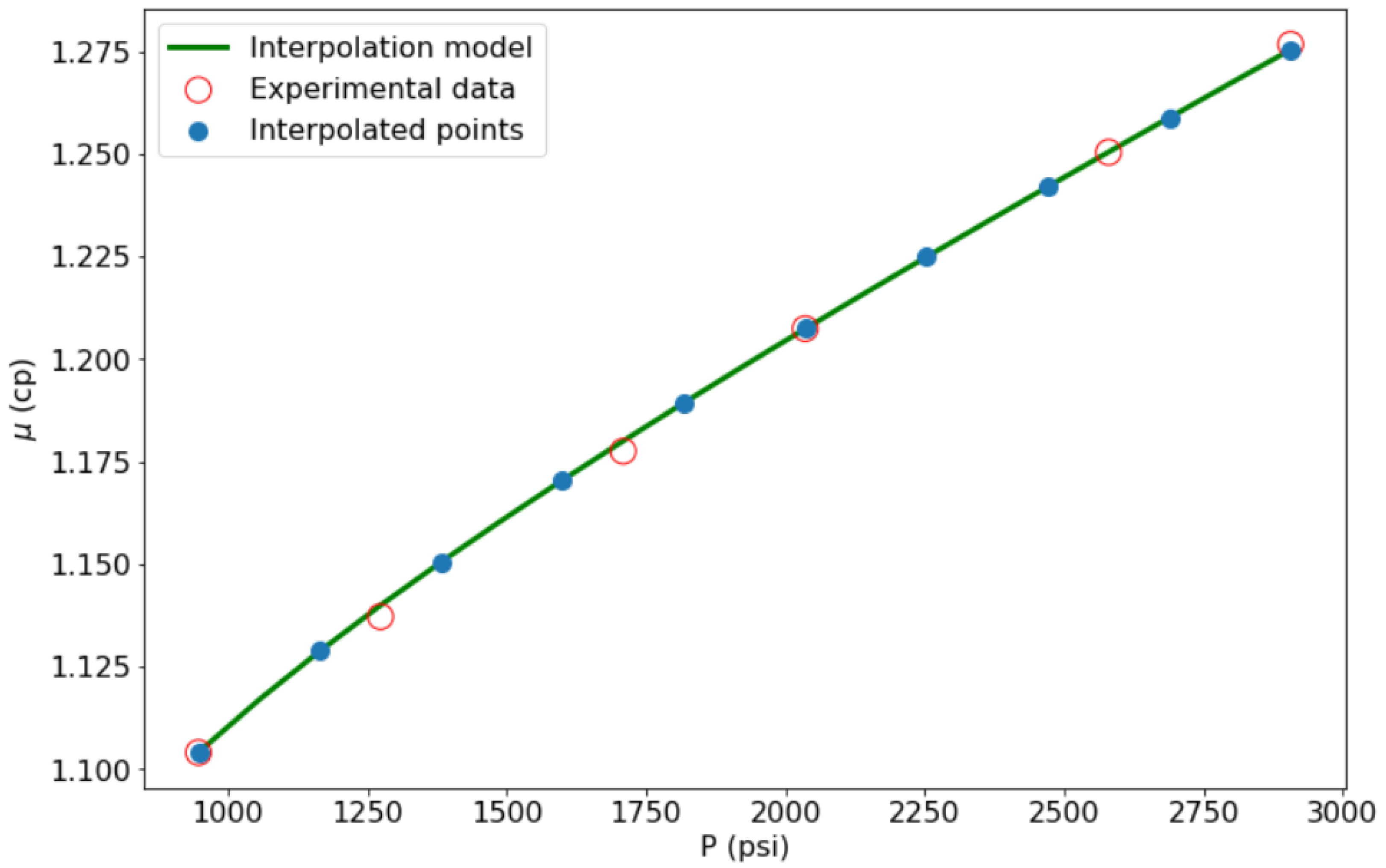
To avoid introducing bias to the evaluation process due to the varying number of pressure steps between $P_b$ and $P_i$ per fluid (which is defined arbitrarily by the PVT lab client), the available measurements were interpolated with fluid-specific first-order rational functions of pressure. Subsequently, each fluid was resampled at a fixed number of pressure values from this curve, equally spaced between $P_b$ and $P_i$, as shown in Figure 1. These rational equations are a result of non-linear regression. In total, twenty points were selected for each fluid between the pressure values stated above.

The range spanned by the cleaned dataset’s undersaturated fluids properties are given in

Table 6. Database fluid properties range.

Parameter	Minimum	Maximum
${\mu }_{ob}\left(cp\right)$	$0.04$	48
$\mu \left(cp\right)$	$0.04$	100
GOR (scf/stb)	0	17,118
API	14	57
$T{(}^{\circ }F)$	87	376
$P_b\left(psi\right)$	36	7303
$P\left(psi\right)$	36	12,750

. Their distribution is further illustrated in the histograms in Figure 2, where the vertical axis corresponds to the percentage of each value bin.

Judging from the distribution of the $P_b$ values in Figure 2, the fluids database utilized contains reservoir fluids, whose saturation pressure is as low as less than a hundred psi, whereas others’ top at 6500 psi, thus exhibiting the fluid-type variance of the dataset. Regarding the oil’s volatility, GOR ranges from nearly zero, i.e., fluids characterized mainly by their C7+ fraction, up to 17,000 scf/stb, a value associated with very highly volatile, near critical fluids. Similarly, API gravity values range from 14 to 50+. It is also shown that the reservoirs’ temperature, which also affects viscosity strongly, is distributed in a wide range spanning from less than ${100}^{\circ }F$ up to more than ${350}^{\circ }F$.

To facilitate the interpretation of the obtained results, the data were further split into four ranges according to the bubble-point viscosity value, as shown in Figure 3. The first and second ranges (0–1 cp and 1–5 cp) can be described as low or mildly viscous fluids, while the third and fourth (5–20 cp and 20–50 cp) correspond to fluids that are highly viscous and do not flow as easily and fast. The number of fluids in each range is shown in the bottom-most part of the Figure 3 in the form of a histogram. The box plots above the histograms indicate the distribution of every input in each range, with the red line in the middle showing the average value and the edges of the box corresponding to the 25th and 75th percentiles. Beyond the box are the whiskers, the end points of which denote the min and max values of the property. As reasonably expected, as bubble-point viscosity increases, API, GOR, $P_b$ and even temperature become low. Interquartile ranges are sometimes high, but this is very common when dealing with PVT values in real-world reservoir oil datasets. Variation also decreases in those properties, but that should probably be attributed to the fewer points in the high viscosity ranges.

4. Results

The evaluation of the correlations’ performance against this dataset is discussed in this section, and results are presented following the grouping defined in Section 2. The typical metrics utilized in the evaluation process are the ARE or Average Relative Error as a measure of bias and AARE or Absolute Average Relative Error as a measure of variance. They are defined as follows:

$$\begin{array}{cc}\hfill & \mathrm{ARE}\% =100·\overline{e}={\displaystyle \frac{100}{N}}\sum _{i=1}^N{e}_i={\displaystyle \frac{100}{N}}\sum _{i=1}^N{\displaystyle \frac{{\left(\widehat{{\mu }_o}\right)}_i-{\left({\mu }_o\right)}_i}{{\left({\mu }_o\right)}_i}}\hfill \\ \hfill & \mathrm{AARE}\% =100·\overline{\left|e\right|}={\displaystyle \frac{100}{N}}\sum _{i=1}^N\left|e_i\right|={\displaystyle \frac{100}{N}}\sum _{i=1}^N\left|{\displaystyle \frac{{\left(\widehat{{\mu }_o}\right)}_i-{\left({\mu }_o\right)}_i}{{\left({\mu }_o\right)}_i}}\right|\hfill \end{array}$$

where $\widehat{\mu }$ is the predicted viscosity value and $\mu$ is the lab-measured one, N is the number of data points considered and $e_i$ is the error of every point. The bar operator is used to note the average value. To evaluate how widely ARE and AARE values are distributed around their means, their standard deviation (SDRE and SDARE) is provided as well, defined by

$$\begin{array}{cc}\hfill & \mathrm{SDRE}\% ={\sigma }_e=\sqrt{{\displaystyle \frac{{\sum }_{i=1}^N{\left(e_i-\overline{e}\right)}^2}{N-1}}}\hfill \\ \hfill & \mathrm{SDARE}\% ={\sigma }_{\left|e\right|}=\sqrt{{\displaystyle \frac{{\sum }_{i=1}^N{\left(|e_i|-\overline{\left|e\right|}\right)}^2}{N-1}}}\hfill \end{array}$$

Lastly, Pearson’s correlation coefficient ($R^2$) is used as a simple metric of the match between measured and predicted viscosity values, defined by

$$R_{X,Y}^2={\displaystyle \frac{\overline{({\mu }_o-\overline{{\mu }_o})(\widehat{{\mu }_o}-\overline{\widehat{{\mu }_o}})}}{{\sigma }_{{\mu }_o}{\sigma }_{\widehat{{\mu }_o}}}}$$

where ${\sigma }_{{\mu }_o}=\sqrt{{\displaystyle \frac{{\sum }_{i=1}^N{\left({\left({\mu }_o\right)}_i-\overline{{\mu }_o}\right)}^2}{N-1}}}$, ${\sigma }_{\widehat{{\mu }_o}}=\sqrt{{\displaystyle \frac{{\sum }_{i=1}^N{\left({\left(\widehat{{\mu }_o}\right)}_i-\overline{\widehat{{\mu }_o}}\right)}^2}{N-1}}}$.

Results are presented separately for each cluster of correlations, so as to enhance readability and allow for direct comparisons. Their visualization is attempted in Figure 4, Figure 5, Figure 6, Figure 7 and Figure 8. ARE and AARE are plotted per group/cluster and per viscosity value range to allow for the evaluation of the correlations’ performance on various oil types. The correlation performance data series are slightly shifted to each other to avoid overlapping and facilitate comparison. Some markers are hollow, indicating that the corresponding correlation is being tested outside its design inputs range. For example, Petrosky’s correlation exhibits ARE and AARE errors of approximately $-24\%$ and $-26\%$ when tested against the data points with viscosity in the 5–20 cp and 20–50 cp, respectively. However, as indicated by the hollow points, that result is not representative of the correlation value, as the latter is tested beyond its design range.

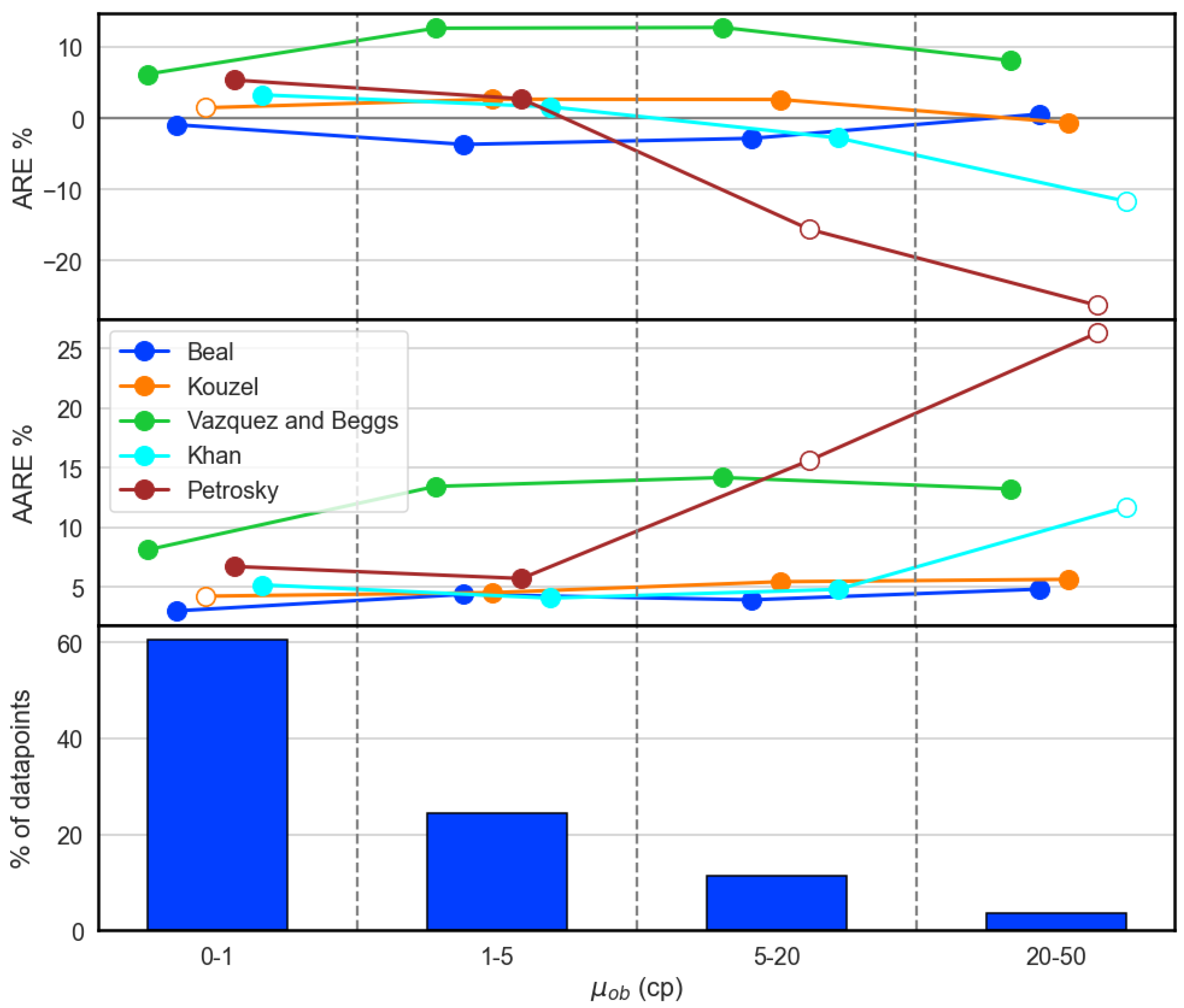
In Figure 4 (cluster $A_1$) it is notable that the Beal and Kouzel models produce almost no systematic error at all for the full viscosity values range, with Beal’s model performing marginally better in terms of AARE. Khan’s model was a close match up until tested against values above its design limit (i.e., 20–50 cp). This did not hinder Kouzel’s model performance regarding its prediction against low ${\mu }_o$ values below its design range. Petrosky’s correlation suffers from similar issues as Khan’s, while the correlation of Vazquez and Beggs performs consistently below average across all ranges. Note that all of these correlations share the same form $\mu =f({\mu }_{ob},P,P_b)$.

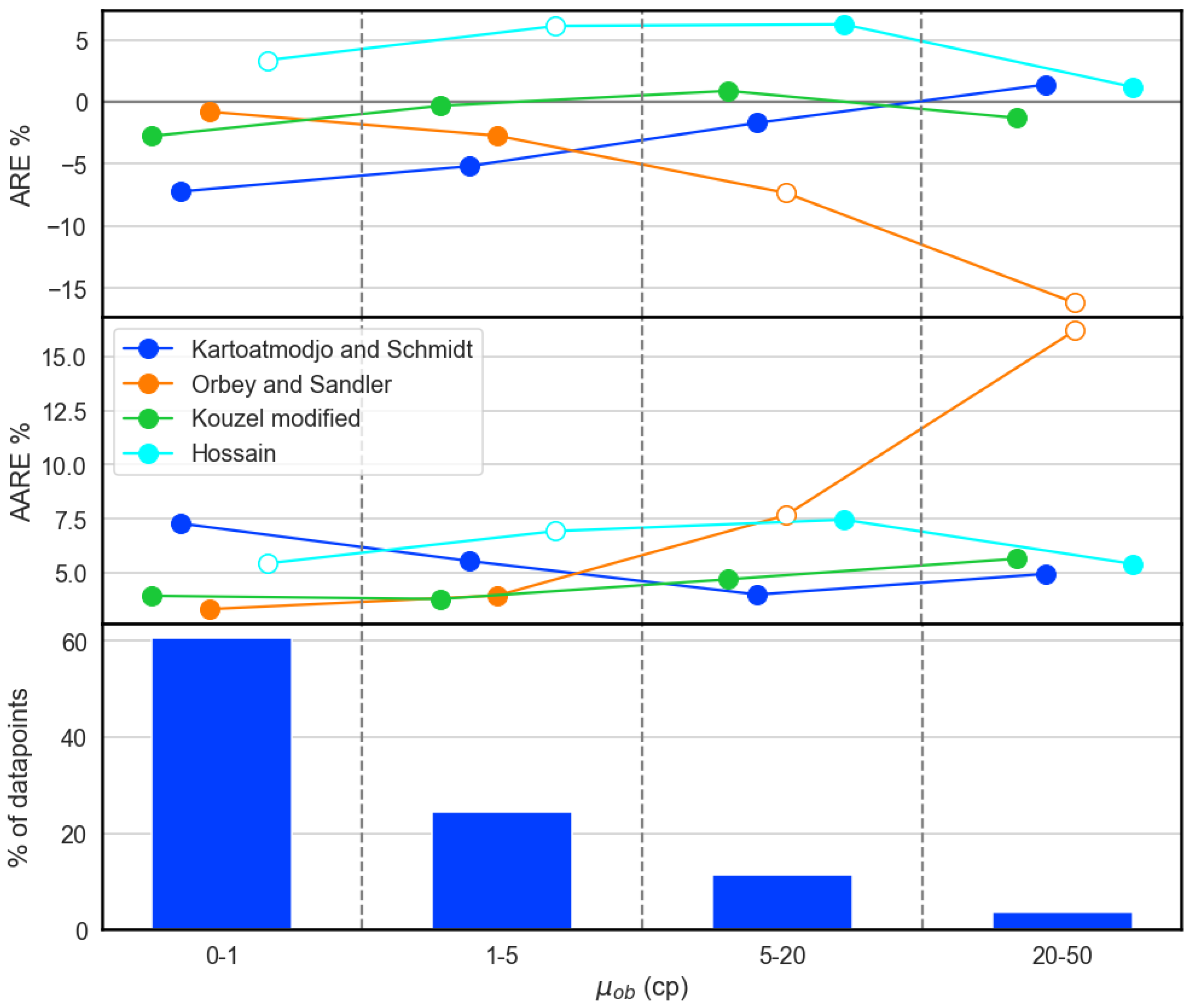
Figure 5 depicts the performance of the second correlations set of the form $\mu =f({\mu }_{ob},P,P_b)$, namely cluster $A_2$. The modified Kouzel correlation and those by Hossain and Kartoatmodjo all seem to reach a level of being unbiased as viscosity increases, as opposed to cluster $A_1$, where most models only start off as unbiased. Hossain’s is the only one that performs better above the 5 cp limit, which is reasonable since the latter is within its design range. Orbey and Sandler’s model performs similarly to Petrosky’s, severely underestimating values when above its designed viscosity range.

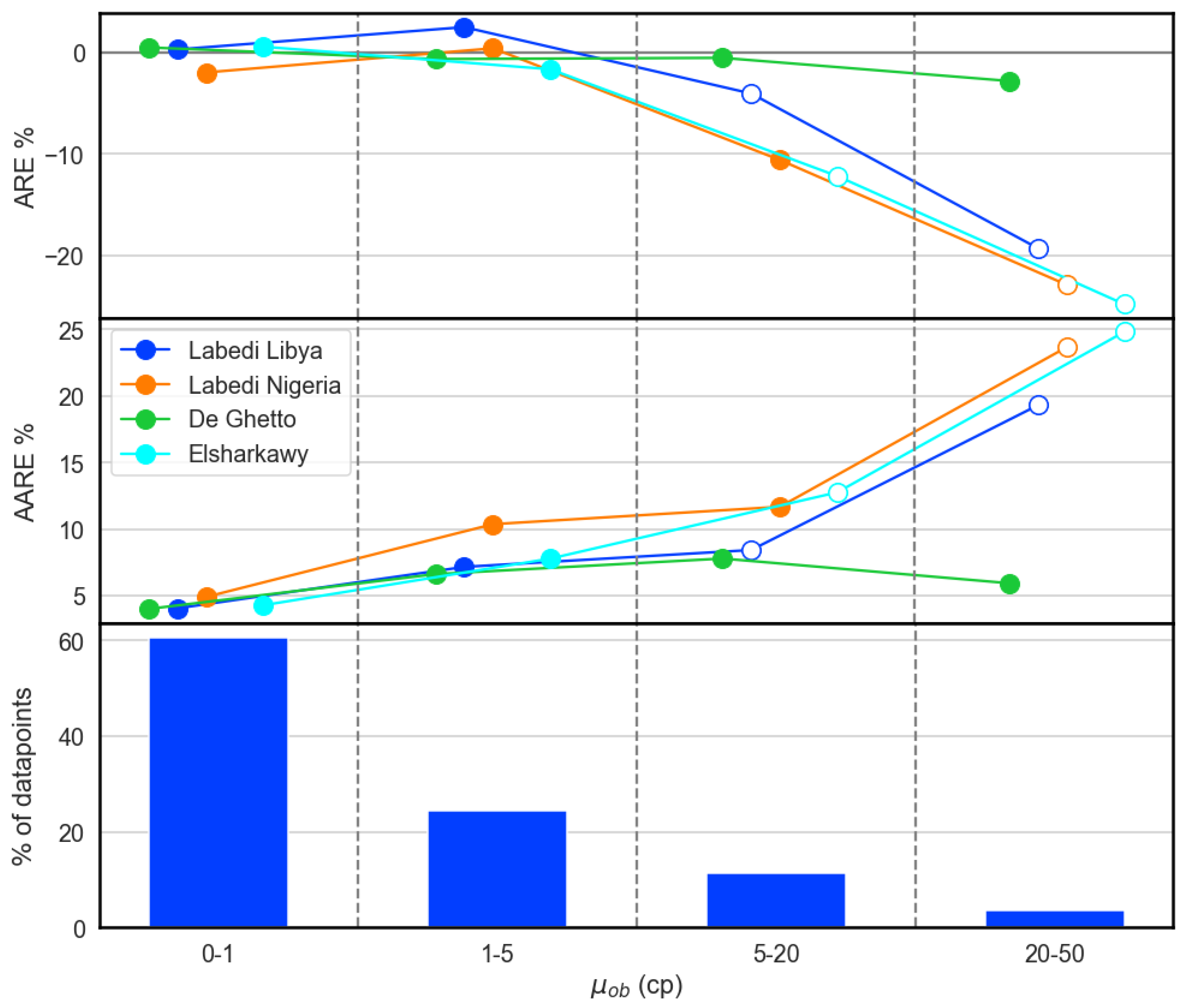
Figure 6 illustrates the results obtained for correlations in cluster $B_1$ which further utilize dead oil viscosity and share the common form of $\mu =f({\mu }_{ob},P,P_b,{\mu }_{od},GOR,API)$. Most dead oil viscosity values are not available in the dataset and were estimated using Beggs and Robinson correlation [30], which considers oil API and reservoir temperature in the following form:

$$\begin{array}{cc}\hfill & {\mu }_{od}={10}^x-1\hfill \\ \hfill & x={10}^{3.0324-0.02023·API}·T^{-1.163}\hfill \end{array}$$

It should be noted that this approach is common practice to estimate ${\mu }_{od}$, as its lab measurement requires that a full viscosity study needs to be run which, unlike a single measurement of ${\mu }_{ob}$, severely increases the analysis cost. Labedi’s correlation for Nigerian oils generally performs worse than his Libya model, despite the first being built against a wider range of viscosity values. Elsharkawy’s model completely underestimates values above its design limit, just like Petrosky’s does. De Ghetto’s correlation seems to have lowest bias in the bunch, which should probably be attributed to the fact that De Ghetto’s model does not utilize dead oil viscosity for a certain range of API values. Clearly, all models but the one by De Ghetto cannot perform for oils of high viscosity above 5 cp.

The correlations in cluster $B_2$, Figure 7, are of the form $\mu =f({\mu }_{ob},P,P_b,GOR,API)$. Dindoruk’s model performs poorly above its design range but very accurately inside that. Abdul-Majeed’s correlations produced extremely high errors for GOR values below 50 scf/stb, and these fluids were not included in the latter’s evaluation to avoid receiving unrealistic statistics. Al-Khafaji’s model suffers from the same drawbacks as Petrosky’s.

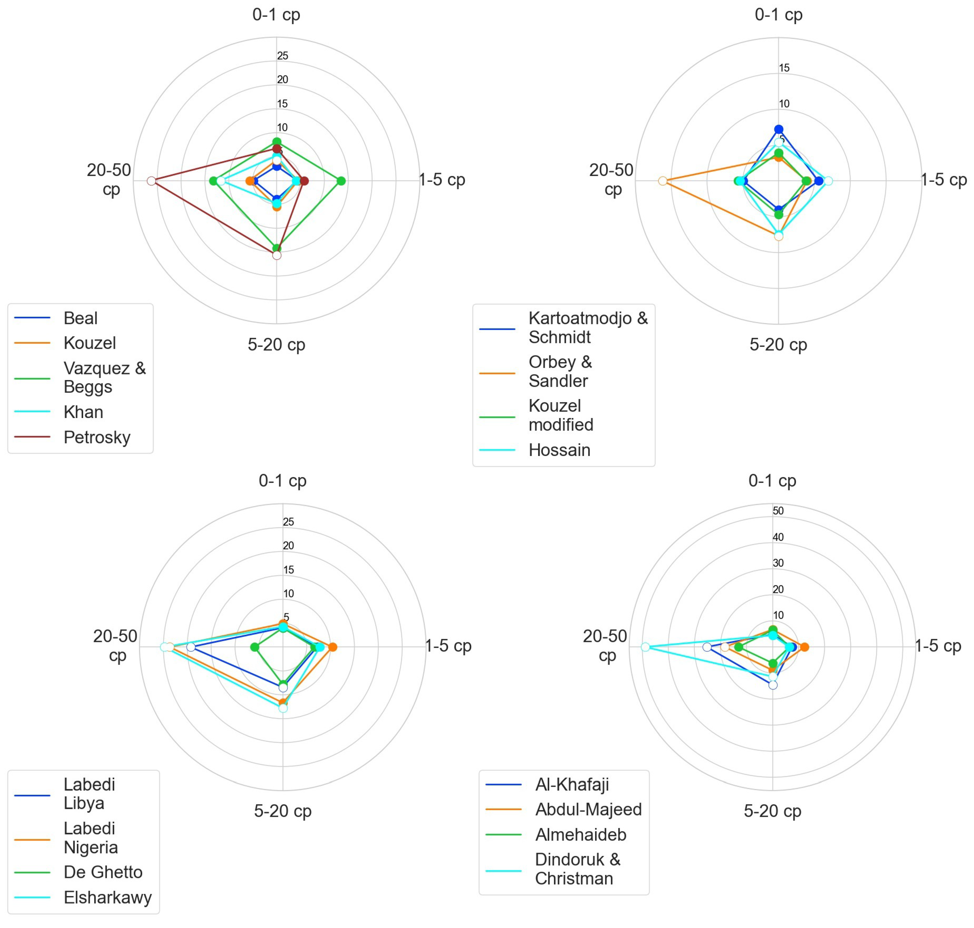
Radar charts showing all correlations AARE are implemented in Figure 8 to allow correlations comparison in a more concise way. It is noted that as was the case with Figure 4, Figure 5, Figure 6 and Figure 7, filled and hollow points indicate correlations acting within or beyond their design range, respectively. It can be readily seen that the models by Beal and Kouzel exhibit far better performance than any other correlation for any fluid in all four ranges. The models by Khan, Vazquez and Beggs and Petrosky exhibit progressively deteriorating accuracy, which becomes more acute the higher the viscosity is. As far as the correlations in cluster $A_2$ are concerned, all but that by Orbey and Sandler exhibit ARE values of less than 10% in all ranges, with the modified Kouzel one being the most accurate, slightly better than the original one appearing in cluster $A_1$.

In cluster $B_1$, all models except De Ghetto’s produce high AARE values with progressing viscosity range. As seen in Table 3, De Ghetto’s model consists of four equations, three of which are modified versions of Labedi’s, and the other being a modified version of Kartoatmodjo’s. From Figure 3, it is apparent that the last ${\mu }_{ob}$ range consists of very low-volatility oils, where fluids have an API value below 20. At this API range, De Ghetto’s equation has a form resembling Kartoatmodjo’s, which itself produces accurate results. This is the main reason justifying De Ghetto’s advantage in the last range. Lastly, regarding cluster $B_2$, Dindoruk and Christman’s correlation performs the best when low-viscosity fluids are considered, but soon, the error increases rapidly outside its design range. Although Al-Khafaji’s and Abdul Majeed’s models do not suffer from the same drawbacks, they provide poor predictions on the first two viscosity ranges. Overall, Almehaideb’s correlation would be the one to choose out of this cluster, as it stays close to 10% AARE, even in the range of 20–50 cp.

The full set of all five metrics discussed at the beginning of Section 4 are given in the Appendix A in

Table A1. Detailed metric values for all correlations and for ${\mu }_{ob}$ range 0–1.

Cluster	Correlation	ARE	SDRE	AARE	SDARE	${\mathit{R}}^2$
$A_1$	Beal (1946)	−0.92	5.07	3.00	4.18	0.993
	Kouzel (1965)	1.46	6.84	4.23	5.57	0.990
	Vazquez and Beggs (1976)	6.18	13.34	8.11	12.26	0.953
	Khan (1987)	3.26	7.70	5.18	6.57	0.987
	Petrosky (1990)	5.36	26.26	6.73	25.94	0.986
$A_2$	Kartoatmodjo and Schmidt (1991)	−7.23	7.16	7.28	7.11	0.987
	Orbey and Sandler (1993)	−0.80	5.75	3.31	4.77	0.993
	Kouzel Modified (1997)	−2.76	6.08	3.93	5.40	0.993
	Hossain (2005)	3.35	7.21	5.43	5.81	0.990
$B_1$	Labedi Nigeria (1982)	−1.96	9.38	4.90	8.23	0.962
	Labedi Libya (1982)	0.31	6.74	4.05	5.40	0.989
	De Ghetto (1994)	0.51	6.65	4.00	5.34	0.990
	Elsharkawy (1999)	0.58	7.60	4.28	6.31	0.983
$B_2$	Al-Khafaji (1987)	−0.23	11.02	4.82	9.91	0.985
	Abdul-Majeed (1990)	1.98	14.92	6.67	13.49	0.929
	Almehaideb (1997)	4.48	11.74	6.42	10.80	0.979
	Dindoruk and Christman (2001)	2.28	6.50	4.45	5.26	0.992

,

Table A2. Detailed metric values for all correlations and for ${\mu }_{ob}$ range 1–5.

Cluster	Correlation	ARE	SDRE	AARE	SDARE	${\mathit{R}}^2$
$A_1$	Beal (1946)	−3.69	5.60	4.39	5.08	0.980
	Kouzel (1965)	2.66	6.81	4.53	5.74	0.980
	Vazquez and Beggs (1976)	12.62	20.51	13.43	19.99	0.914
	Khan (1987)	1.60	6.35	4.07	5.12	0.981
	Petrosky (1990)	2.72	8.09	5.72	6.33	0.976
$A_2$	Kartoatmodjo and Schmidt (1991)	−5.19	6.07	5.54	5.75	0.979
	Orbey and Sandler (1993)	−2.73	5.57	3.95	4.79	0.981
	Kouzel Modified (1997)	−0.32	5.88	3.78	4.52	0.982
	Hossain (2005)	6.11	7.61	6.92	6.88	0.979
$B_1$	Labedi Nigeria (1982)	0.43	19.71	10.37	16.77	0.908
	Labedi Libya (1982)	2.51	13.63	7.16	11.87	0.968
	De Ghetto (1994)	−0.64	12.19	6.62	10.25	0.971
	Elsharkawy (1999)	−1.64	12.27	7.78	9.62	0.963
$B_2$	Al-Khafaji (1987)	−7.06	7.41	7.51	6.95	0.973
	Abdul-Majeed (1990)	8.92	25.79	12.28	24.37	0.890
	Almehaideb (1997)	2.39	9.90	6.54	7.81	0.966
	Dindoruk and Christman (2001)	5.39	7.04	6.40	6.14	0.980

,

Table A3. Detailed metric values for all correlations and for ${\mu }_{ob}$ range 5–20.

Cluster	Correlation	ARE	SDRE	AARE	SDARE	${\mathit{R}}^2$
$A_1$	Beal (1946)	−2.84	5.83	3.93	5.16	0.989
	Kouzel (1965)	2.62	7.35	5.45	5.58	0.985
	Vazquez and Beggs (1976)	12.73	22.86	14.17	22.00	0.871
	Khan (1987)	−2.78	6.44	4.80	5.10	0.988
	Petrosky (1990)	−15.60	10.87	15.60	10.87	0.942
$A_2$	Kartoatmodjo and Schmidt (1991)	−1.69	5.87	3.99	4.63	0.989
	Orbey and Sandler (1993)	−7.35	6.91	7.66	6.55	0.983
	Kouzel Modified (1997)	6.62	4.69	4.75	0.987
	Hossain (2005)	6.25	7.90	7.45	6.77	0.985
$B_1$	Labedi Nigeria (1982)	−10.59	10.04	11.67	8.76	0.95
	Labedi Libya (1982)	−4.03	11.93	8.43	9.35	0.942
	De Ghetto (1994)	−0.52	15.91	7.79	13.89	0.871
	Elsharkawy (1999)	−12.18	9.93	12.76	9.18	0.954
$B_2$	Al-Khafaji (1987)	−14.20	10.52	14.50	10.09	0.949
	Abdul-Majeed (1990)	−0.82	13.72	8.96	10.43	0.934
	Almehaideb (1997)	−1.72	8.94	6.20	6.67	0.968
	Dindoruk and Christman (2001)	10.89	9.41	11.37	8.83	0.986

and

Table A4. Detailed metric values for all correlations and for ${\mu }_{ob}$ range 20–50.

Cluster	Correlation	ARE	SDRE	AARE	SDARE	${\mathit{R}}^2$
$A_1$	Beal (1946)	0.56	7.65	4.82	5.97	0.968
	Kouzel (1965)	−0.66	7.91	5.64	5.58	0.964
	Vazquez and Beggs (1976)	8.09	20.50	13.22	17.63	0.862
	Khan (1987)	−11.66	8.28	11.67	8.27	0.958
	Petrosky (1990)	−26.27	14.49	26.27	14.49	0.792
$A_2$	Kartoatmodjo and Schmidt (1991)	1.39	7.61	4.94	5.95	0.968
	Orbey and Sandler (1993)	9.92	16.20	9.92	0.936
	Kouzel Modified (1997)	7.73	5.65	5.43	0.964
	Hossain (2005)	1.20	7.49	5.41	5.32	0.968
$B_1$	Labedi Nigeria (1982)	−22.90	14.85	23.66	13.60	0.802
	Labedi Libya (1982)	−19.30	12.27	19.30	12.27	0.874
	De Ghetto (1994)	−2.80	7.41	5.93	5.25	0.967
	Elsharkawy (1999)	−24.81	14.03	24.81	14.03	0.818
$B_2$	Al-Khafaji (1987)	−25.30	13.69	25.30	13.69	0.829
	Abdul-Majeed (1990)	−18.28	11.80	18.28	11.80	0.914
	Almehaideb (1997)	−7.63	14.63	13.08	10.05	0.872
	Dindoruk and Christman (2001)	47.42	40.03	48.98	38.10	0.953

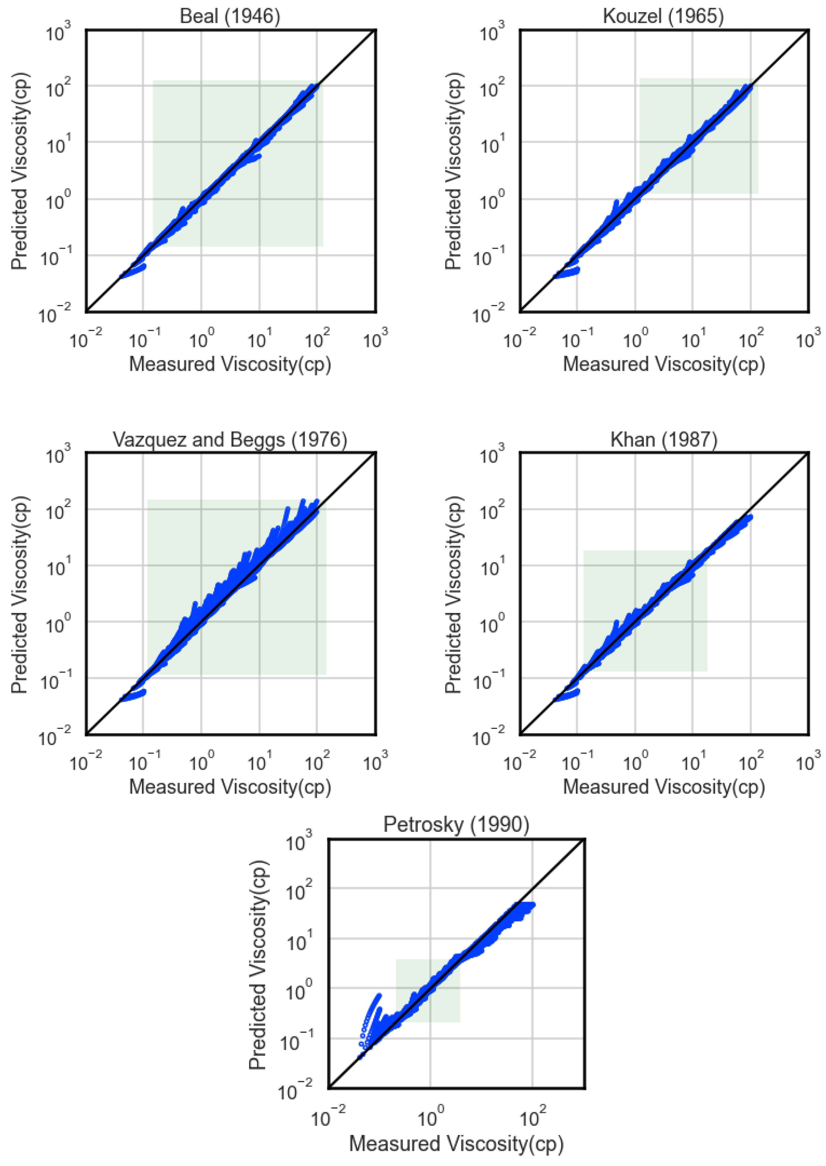
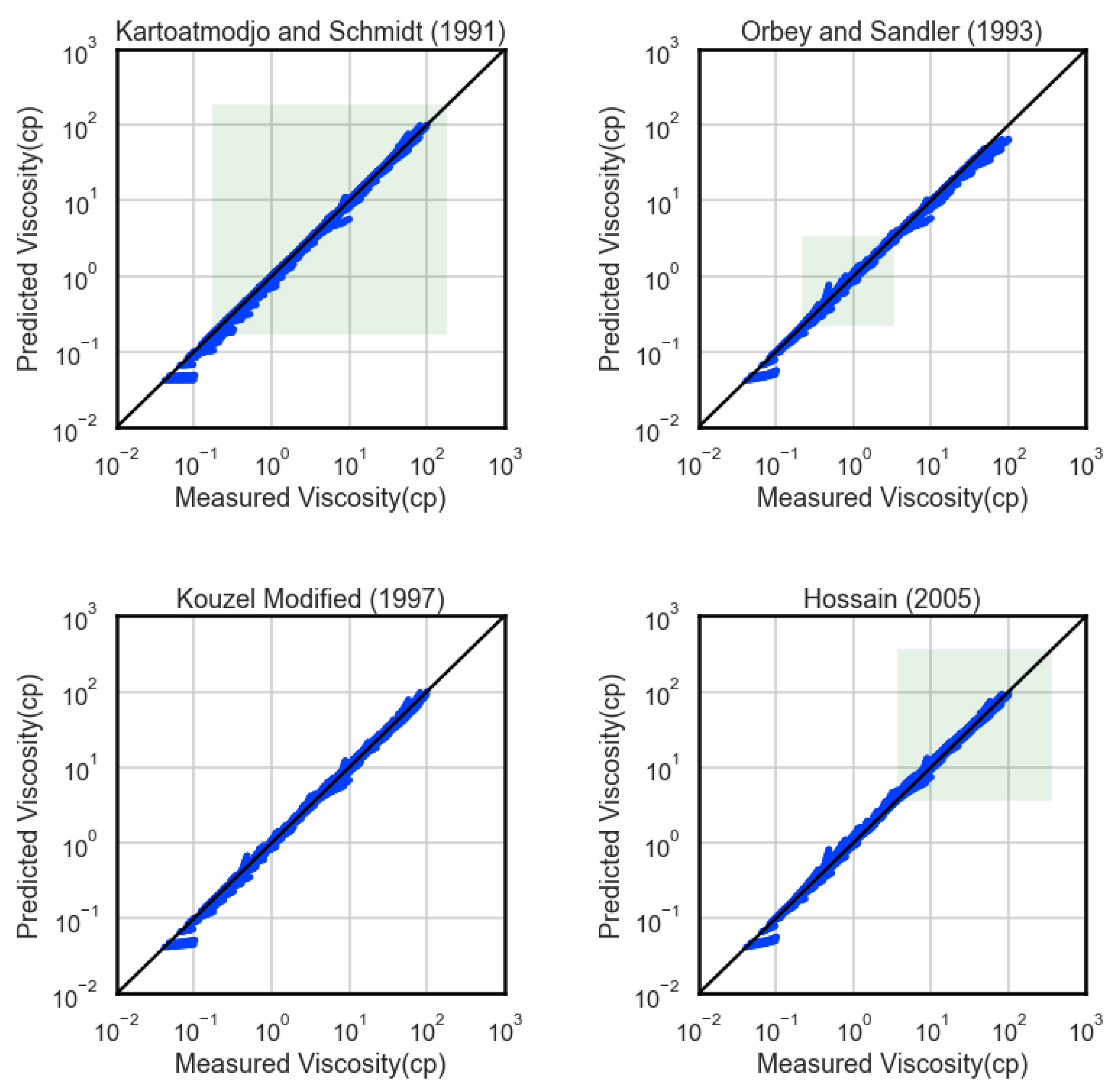
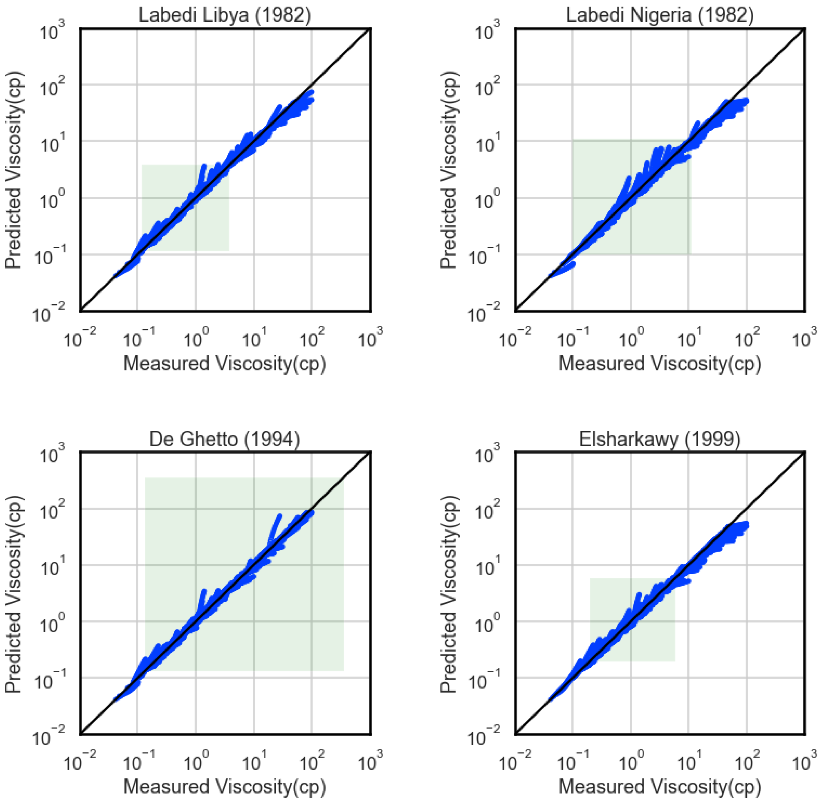
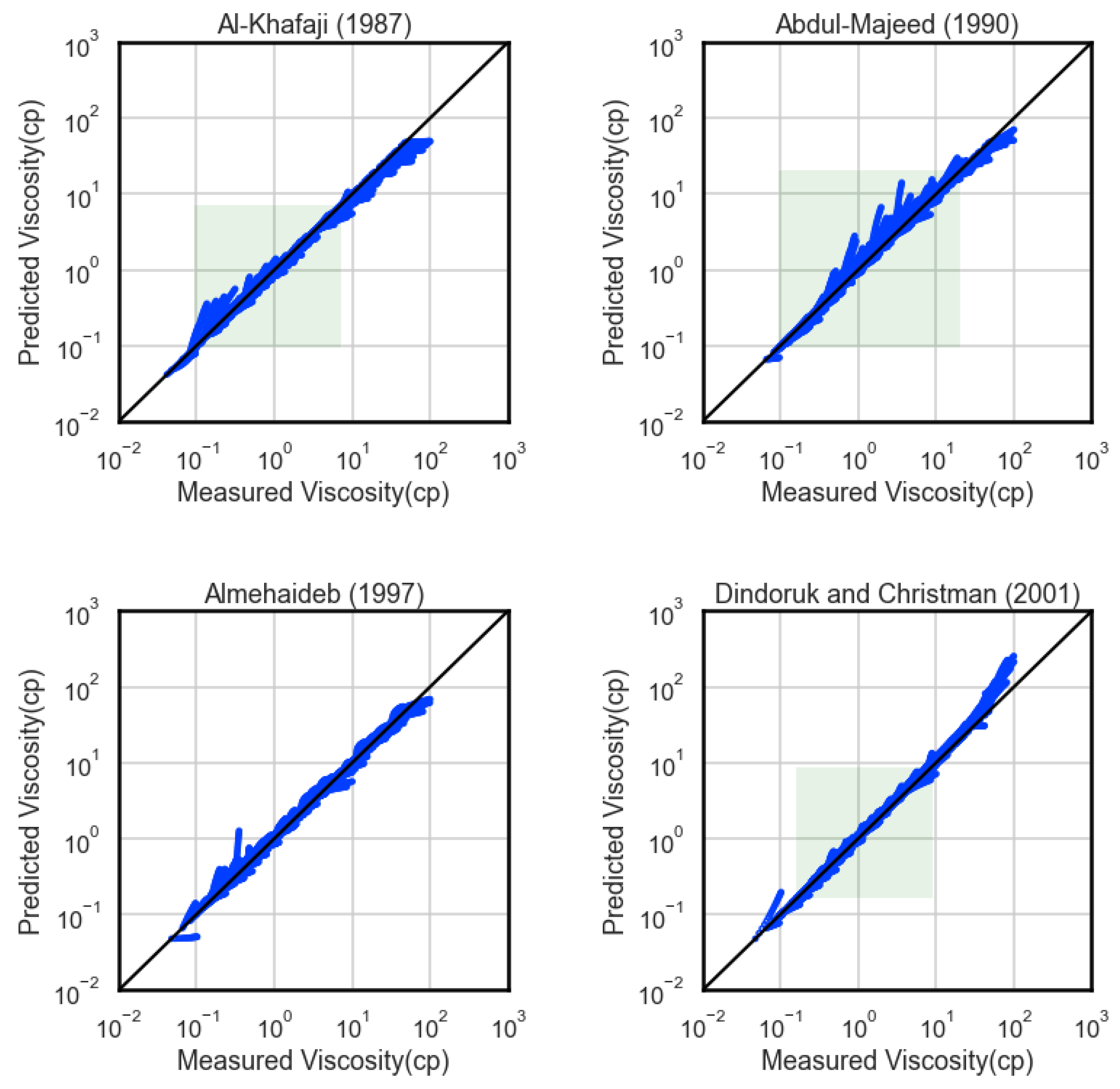
for the four distinct viscosity values ranges discussed above, following the policy of similar publications. Green highlighting is used to indicate that the corresponding correlation is evaluated within its design range. The same convention is used in Appendix B regarding the parity plots, where the experimentally measured viscosity values are shown in scatter plots vs the model-predicted ones. In these plots, a green box is used to indicate the space of bubble-point viscosity values inside which the corresponding correlation was developed. As the Tables progress towards ranges of increasing viscosity, it can be verified that correlations in the white background appear more often and perform worse than those in the green.

An overall comparison of their performance for all ranges reveals that most correlations perform very well in the first range of bubble-point viscosity (0-1 cp) that corresponds to oils of medium-to-high volatility. On the other hand, they perform excessively badly in the range of the highly viscous fluids, but only if their development range is way below these values. They all tend to underestimate viscosity values in this range, thus being negatively biased. Closer examination shows that their formulas are generated in a way that forbids predicted viscosity to change according to pressure change in that region.

5. Discussion

Although physical evidence exists that could have been used to develop physics-driven models (such as the facts that undersaturated reservoir oil has constant composition, lies in a single liquid phase, the reservoir’s temperature is constant and pressure change does not really bring the molecules significantly closer together in liquids since they are incompressible), the reservoir engineer community still relies on data-driven models such as the ones presented in this work. Strictly speaking, the only principle embedded in all models’ mathematical form is that oil viscosity increases with pressure. 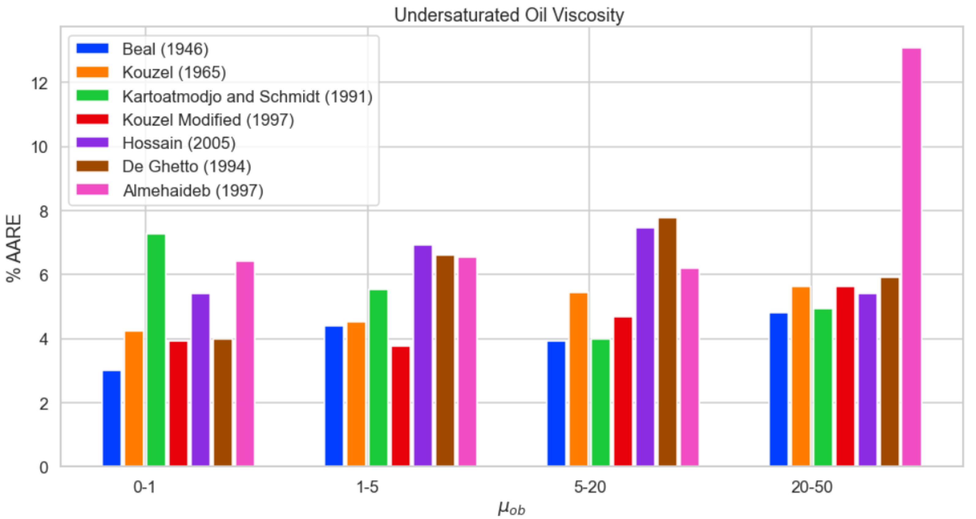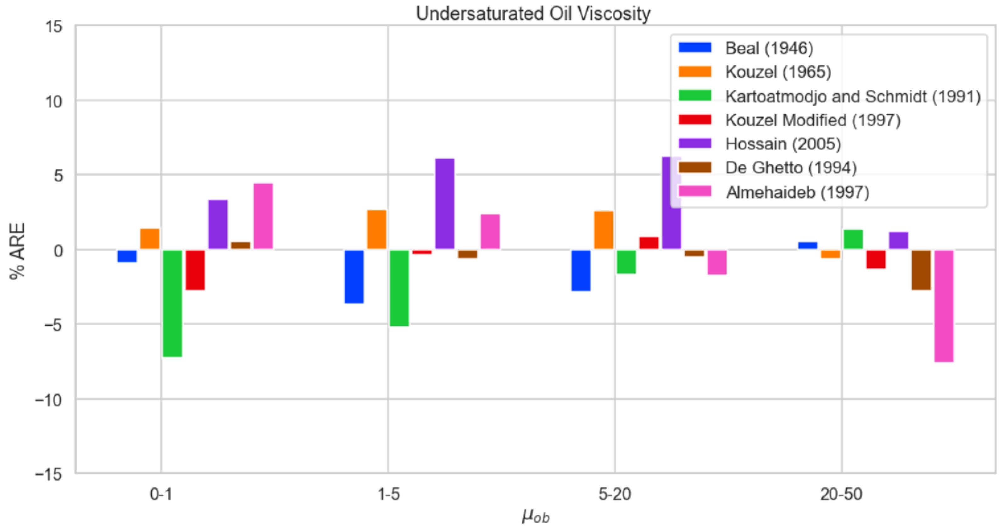As a result, the performance compared in Figure 9 and Figure 10 has only been a result of the developers’ skills and the dataset used, rather than the physics principles considered.

By comparing in detail all correlations, an ordering of their performance for various fluid types can be achieved to address the question of the most accurate correlation that should be used. For this purpose, two workflows are considered to identify the most appropriate correlation when a single model or various models along different ranges might be used, subject of course to their availability in the flow simulator utilized. For the first task, where a single correlation is sought, Beal’s correlations outperforms all others at every viscosity range, and it should be hands down the first choice to use when available in the software package used. It is closely matched by Kouzel’s modified and Kouzel’s original model. Finally, De Ghetto’s correlation would be the fourth best in order when it comes to overall performance. The ordering, however, may be altered according to the task at hand, regarding bubble-point viscosity range or even the locality of the fluid that is being studied.

For applications where different correlations may be combined according to the ${\mu }_{ob}$ value, Figure 9 and Figure 10 provide an insight as to which correlation performs best at each range by comparing the metrics ARE and AARE between the top performing correlations. In the first range (0–1 cp), it is Beal’s correlation that achieves the lowest AARE, and it is De Ghetto’s one that achieves the least bias. In the second range (1-5 cp), the modified Kouzel equation is clearly the top performer among both metrics. Regarding the third (5–20 cp) and fourth range (20–50 cp), Beal’s equation is once again the best performer in terms of AARE, while being closely matched by Kartoatmodjo’s one. In the third range, however, De Ghetto’s correlation is once again the most unbiased, while in the fourth range there is a handful of correlations that achieve this goal.

This study provides an in-depth analysis of the suitability of known correlations for the prediction of undersaturated oil viscosity against hundreds of never seen before fluids. It is complete in the sense that it gives a strong indication as to which correlations should be applied when using flow simulating software. The large number of datasets utilized provide a sense of security to the engineer when they try to make a prediction of the evolution of the viscosity in a reservoir. The negative aspect of this study is mainly the minimal usage of experimental dead oil viscosity data, giving a handicap to several correlations in terms of judging their true performance. Additional research is needed to determine a model that performs optimally in all classes, and the abundance of data points in our disposal may lead to a new model. This model may be a result of regression analysis or more complex machine learning techniques.

6. Conclusions

A thorough examination and evaluation of correlations for the prediction of underasturated oil viscosity was presented, followed by a fair comparison process which guarantees that the correlations were judged appropriately.

The metrics obtained through this process show that a method should be chosen only when the task at hand is within the method’s design range. Users also have to consider the locality of the fluids in which they work on in order to choose between similarly performing correlations. In general, linear in $\mathsf{\Delta }P$ models tend to predict experimental values with better accuracy, although the curvature of ${\mu }_{ob}$ with respect to P is ignored. Surprisingly, one of the oldest models (Beal 1946) performed on average better than most newer ones, even the ones developed in the 2000s. Models of the second group (clusters $B_1$ and $B_2$) performed worse than those in the first one, despite their enhanced input, but still, given the correct data, some may find success in trying out the top performers of each cluster. The above analysis was coded in guidelines/workflows which can be used by engineers facing the problem of choosing the most suitable model for their task at hand.