Abstract
The direct reduction process has been developed and investigated in recent years due to less pollution than other methods. In this work, the first direct reduction iron oxide (DRI) modeling has been developed using artificial neural networks (ANN) algorithms such as the multilayer perceptron (MLP) and radial basis function (RBF) models. A DRI operation takes place inside the shaft furnace. A shaft furnace reactor is a gas-solid reactor that transforms iron oxide particles into sponge iron. Because of its low environmental pollution, the MIDREX process, one of the DRI procedures, has received much attention in recent years. The main purpose of the shaft furnace is to achieve the desired percentage of solid conversion output from the furnace. The network parameters were optimized, and an algorithm was developed to achieve an optimum NN model. The results showed that the MLP network has a minimum squared error (MSE) of 8.95 × 10⁻⁶, which is the lowest error compared to the RBF network model. The purpose of the study was to identify the shaft furnace solid conversion using machine learning methods without solving nonlinear equations. Another advantage of this research is that the running speed is 3.5 times the speed of mathematical modeling.
1. Introduction
Direct reduction of iron oxide (DRI) is one of the most important non-catalytic gas-solid reactions in industry, and it continues to be an important field of study in chemical engineering [1,2]. The MIDREX process, which is one of the direct-reduction technologies, has received a lot of interest because it is a great technology for considerably reducing carbon dioxide (CO2) emissions from steel plants [3,4]. This is primarily accomplished by using natural gas instead of coke or coal [5]. Several approaches were used to develop these solutions, whose overview is provided in Figure 1.
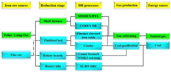
Figure 1.
Direct reduction methods have been developed extensively [6].
Despite the global COVID-19 pandemic, global DRI output in 2020 is 104.4 million tonnes which has a 3.4% decrease compared with the previous year’s record of 108.1 million tonnes. India and Iran produced about half of the world’s DRI [7].
The shaft furnace, reformer, and recuperator are the three main parts of the Midrex process, of which the shaft furnace is the most important. Within the shaft furnace, reduction processes take place, and iron oxide turns into sponge iron. Researchers have recently worked to regenerate hydrogen and develop the new MIDREX process design. Pimm et al. improved the MIDREX process to use renewable energies to satisfy the energy needs of the revised MIDREX process and the hydrogen-based MIDREX unit. According to Rechberger et al.’s research, the carbon footprint of the power used to manufacture hydrogen has a significant impact on the amount of potential that the hydrogen-based pathway offers for environmentally friendly steelmaking [8,9].
Figure 2 indicates direct reduction processes for the production of sponge iron which uses natural gas as the major reducing agent. Today these processes provide for more than 70% of the overall production of DRI and hot briquetted iron (HBI). Natural gas is transformed into reducing agents, mostly carbon monoxide and hydrogen, which operate as iron oxide reducers [6]. The shaft furnace is divided into three main parts: (i) reduction zone, (ii) transition zone, and (iii) cooling zone. The most fundamental part of the shaft furnace is the place where reduction occurs. Therefore, most of the modeling has been conducted around this area. The unreacted shrinking core model (USCM) is an assumption adopted by the majority of prior simulations at the pellet scale [10,11,12]. Furthermore, some modeled direct reduction reactors in industrial units use this model and achieved desirable results [13,14]. Nevertheless, the grain model can be better than the USCM at predicting plant data [15].
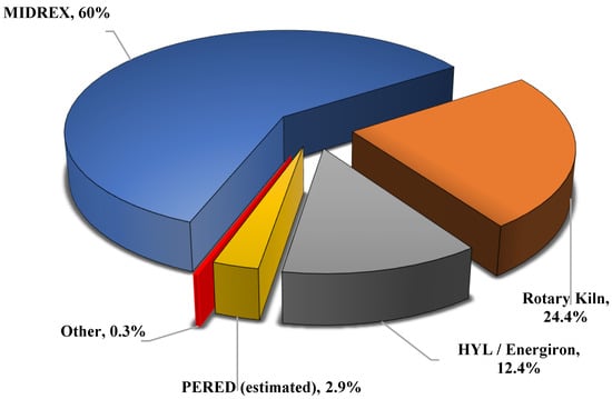
Figure 2.
World DRI Production report (2020) using different technologies [7].
Hamadeh et al. assumed that the shaft furnace had pellets made of grains and crystals [4]. In some reactor models, only one reductant gas is used, such as pure H2 gas [12,16,17,18], pure CO gas [19,20], and H2 and CO mixtures [21,22]. In a real shaft furnace, the reducing gas is a combination of H2, CO, H2O, CH4, and CO2 [4]. Modeling and simulation of industrial direct reduction furnaces have been performed by numerical solutions and computational fluid dynamics (CFD), which are summarized in Table 1. Additionally, some notable non-industrial modeling is given in Table 2.
It is employed at research centers today to comprehend the uses of machine learning (ML) in both the present and the future of energy systems. One of the most effective techniques employed in a variety of industrial fields is the deployment of ML algorithms. Because hybrid approaches take advantage of two or more ways to make an accurate forecast, they sometimes yield greater results than a single method. In light of this, it is advised to use hybrid ML strategies in the future [23,24,25].

Table 1.
Summarized simulation works were validated using industrial plants.
Table 1.
Summarized simulation works were validated using industrial plants.
| Authors | Modeling/Simulation | Shaft Furnace Name | Remark | Reference |
|---|---|---|---|---|
| Parisi and Laborde | USCM/Numerical (Rung–Kutta and Dormand–Prince) | Gilmore Siderca | The model fits the data from two MIDREX plants successfully. Furthermore, they enable investigation of the reactor’s behavior under various operating situations. In terms of metallization, it has been determined that if it increases to 100 (a 6 increase in metallization), the output must reduce to 70 (A 30% loss in production). | [13] |
| Valipour and Saboohi | USCM/CFD (FVM) | Gilmore | They concluded that hematite was reduced entirely to magnetite during the reduction of the haematite pellets in a shaft furnace. However, wustite was transformed into iron in the lower section of the bed. Additionally, magnetite was changed into wustite in the center of the bed. Because there was more hydrogen in syngas than carbon monoxide, endothermic reactions were avoided, and as a result, the temperature along the bed was reduced. | [26,27] |
| Nouri et al. | USCM and Grain model with product layer resistance/Numerical Rung–Kutta | Mobarakeh | The impact of reducing gas parameters and pellet properties on the degree of reduction has been examined. They observed that the grain model predicted plant data better than the shrinking unreacted core model. Their calculations demonstrate that even at the lowest flow rate, the Sherwood number is large enough to eliminate the mass transfer resistance effectively. | [15] |
| Alamsari et al. | USCM/CFD (FEM) | Krakatau | The increase in H2 composition is predicted, whereas the attenuation of CO results in a higher metallization degree. The degree of metallization increases as the gas inlet temperature rises. It was discovered that lowering the gas temperature below 973 °C (1246 K) is not suggested because sticky iron production would occur. They also investigated the impact of lowering the iron’s temperature on the generation of total carbon in the cooling zone and isobaric iron reactor. | [28] |
| Khalid Alhumaizi et al. | USCM/Numerical (Developed computer code) | Saudi Arabia | The simulation of a complete MIDREX unit (shaft furnace, reformer, and recuperator) and the study of complex mass–energy interactions between the reformer and the reduction furnace were investigated in an iron plant based on MIDREX technology. According to their parametric study, the scrubber’s exit temperature might be lowered in order to create sufficient water vapor to avoid carbon formation, subject to the limitations placed on preventing carbon deposition in the reformer tubes. The same constraint should apply to the optimization of the recycle ratio. The ratio of natural gas to iron ore is optimal. If we want to improve the natural gas flow rate, it is best to do so at the transition zone, where methane breaks down into carbon and hydrogen and boosts metalization and carburization. | [29] |
| Shams and Moazeni | USCM/Numerical (Rung–Kutta and Gill) | Gilmore | Complete shaft furnace simulation (reduction zone, cooling zone, transition zone) and validation using Gilmore unit data. The pressure drop for the reduction zone’s 9.75 m length was demonstrated to be approximately 0.87 bar. The length of the reduction zone is the only length that has any bearing on pressure drop because of the upward gas flow. Methane causes the production of carbon. The final product has a carbon content of 1.4%. A small portion of the cooling gas that helps produce carbon flows upward and mixes with the reducing gas to cool the solid to about 56 °C. | [30] |
| Ghandi et al. | USCM/CFD (FVM) | Mobarakeh Gilmore | It was discovered that using the twin gas injection approach increases the radial average hydrogen concentration. As a result of the addition of a new gas entrance that injects hot and fresh reducing gas, the overall degree of reduction increases when operating a reactor with a dual injection system. | [31] |
| Mirzajani et al. | Three-interface USCM/Numerical (Rung-Kutta- Dormand–Prince) | Khorasan | According to this study, the two factors that impact the conversion of iron oxide are particle size and gas flow rate. This study has several limitations because most industrial data is only available for the top and bottom of the reactor, not all along the reactor. | [14] |
| Hamadeh et al. | Grain model with Crystallite/CFD (FVM) | Contrecoeur Gilmore | A multi-scale approach accurately describes the principal physical, chemical, and thermal phenomena. The moving bed is assumed to be composed of pellets with grain and crystallites. Eight heterogeneous chemical reactions and two homogeneous chemical reactions are also considered. One of their important findings is that they found a central area with a lower temperature and conversion. | [4] |
| Béchara et al. | Grain model/Aspen Plus model (FDM) | Contrecoeur Gilmore | They built the aspen plus model of the DR shaft derived from the REDUCTOR. Reduced CO2 emissions were investigated. Computer-aided optimization was used to adjust a set of ten operating parameters at the same time. The results revealed a 15% improvement over the original emissions for comparable output values. | [3,32] |
| This Study | ML | Gilmore Siderca Khorasan Mobarakeh | The first modeling was performed using ML, SGD, Adam, and LBFG optimization methods and optimization functions, and the best network for modeling was found. |
Table 2.
Summarized simulation works using non-industrial modeling DRI.
Table 2.
Summarized simulation works using non-industrial modeling DRI.
| Authors | Modeling/Simulation | Shaft Furnace Name | Remark | Ref. |
|---|---|---|---|---|
| Hara et al. | Three-interface USCM/Numerical | Pilot Plant | This model is used for the modeling of the variations in the degree of reduction in an experimental shaft furnace with a diameter of 0.1 m and a height of 4.0 m. It has been discovered that the model can accurately simulate the reduction behavior in the furnace and that the rate constants obtained from the simulation calculation of the experimental data are very close to those found in the previous literature on the fundamental research of iron ore pellet reduction. | [33] |
| Szekely and Evanse | Grain model and Pore model/Numerical | Pilot Plant | Part I and II series articles “a structural model for gas-solid reactions with a moving boundary” introduce two porous models for non-catalytic solid and gas reactions. They investigate the effects of porosity, grain size, and temperature on the reduction. | [34,35] |
| Takenaka et al. | Grain model/Numerical (Rung–Kutta and Gill) | Pilot Plant (Commercial-scale) | They concluded that by increasing the temperature of the reducing gas, the gas ratio required to produce the desired degree of reduction of product is decreased, thereby improving the gas economy. When the H/CO ratio of the reducing gas is high, the endothermic process due to reduction with hydrogen occurs more strongly, decreasing the temperature within the furnace and so retarding the reduction. In this case, either the temperature of the reducing gas needs to be raised, or the gas ratio needs to be raised. | [36] |
| Negri et al. | Three-interface USCM/Numerical | Pilot Plant Yanagiya [37] and Takenaka [36]. | The consumption of hydrogen is greater than that of carbon monoxide; this is consistent with the higher reduction rate expected by the given kinetic data for the first reactant. | [22] |
| Usai | Zone and Grain model/Experimental and Numerical | Pilot Plant | Based on the grain model, they explored the isothermal reduction of wustite pellet with hydrogen under pseudo-steady state and unsteady state circumstances. They said that the pseudo-steady state solution of their model performed well when compared to the unsteady state solution. | [18] |
| Kang et al. | USCM/Experimental and Analytical | Pilot Plant | Using Ishida–Mathematical Wen’s model, the effect of the size and form of iron oxide samples during reduction with CO–CO2 mixtures at 800 and 900 °C were discussed. | [38,39] |
| Bonalde et al. | Grain model/Experimental and Numerical | Pilot Plant | Using the grain model, the kinetics of reducing hematite pellets using hydrogen–carbon monoxide mixtures as the reducing agent was characterized. The experimental results were compared to the model’s predictions. | [40] |
| Rahimi and Niksiar | Grain Model/Numerical | Pilot Plant Takenaka [36]. | Their findings indicate that the feed temperature appears to have little effect on reactor performance. On the other hand, it is expected that the incoming gas flow rate will have a significant influence. It has also been explained that the significant interconnection of the reactor’s different zones may prevent general expression. | [41] |
| Ranzani da Costa et al. | Grain model with Crystallite/CFD (FVM) | Pilot Plant | They simulated a two-dimensional model of hydrogen-based DRI. Their results show that the use of hydrogen accelerates the reduction in comparison to the CO reaction, and CO2 emissions would be reduced by more than 80%. They made the REDUCTOR model, which is the most accurate shaft model (2D, 3 zones, 10 reactions). | [42] |
| Ponugoti et al. | USCM/Experimental and Numerical | Pilot Plant | They et al. took a new strategy, solving physical governing equations for the solid phase at the same time as gas phase transport equations. The shrinking core model is used to determine the reaction rate, and the genetic method is used to estimate the parameters for the kinetic term. | [43] |
| Yongliang Yan et al. | Experimental | National Energy Technology Laboratory | This was determined using the iron Fe3O4-to-Fe and FeO-to-Fe, H2 kinetic rate constants (for green hydrogen). The response rate of magnetite to iron was demonstrated. They discovered that the Fe3O4 to Fe reduction is a 1D growth with a slower nucleation rate, but the FeO to Fe reduction is a 1D to 2D development process that occurs more rapidly. | [44] |
The reduction zone is a part of the top of the furnace. The followings are the main chemical reactions that take place in the reduction zone [13,15]:
Before recirculation to another usage, a wet scrubber cleans and cools the gas discharged from the top of the furnace shaft. A compressor pressurizes the top gas, which contains CO2 and H2O, before mixing it with natural gas, preheating, and feeding it into a reformer furnace. Hundreds of reformer tubes that are filled with a nickel catalyst are installed in the reformer furnace. The mixture of the top gas and natural gas is reformed in these tubes to produce reductant gas, which consists of carbon monoxide and hydrogen. The following is the reaction that takes place in the reformer tubes [45]:
After ongoing investigations on modeling, Parisi et al. developed a network for stable solid-state heterogeneous reactors by using neural networks for steam reformers that were able to respond 20 times faster than the numerical model [46]. In another research, a tubular reactor with a fixed bed full of porous pellets was developed isothermally by using an unsupervised grid with an accuracy of approximately 10−9 [47]. The use of ML approaches in the simulation of the shaft furnace to estimate the conversion rate of pellets for making sponge iron can overcome the challenges of using nonlinear modeling and is one of the most important achievements of this research. Due to the complexity of pellet behavior, the difficulty of modeling, and the precise prediction of pellet behavior, a new model has been proposed in this study by using an artificial neural network (ANN). Consequently, Figure 3 presents four fundamental models for the DRI process. The low error value in the ANN method, and the complexity of mathematical modeling caused by the ANN technique, make it interesting.
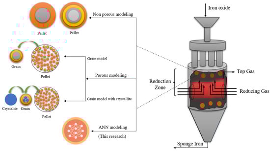
Figure 3.
Models developed for pellets in shaft furnaces [3,17,18,19,30,31,32,33,34,39].
The purpose of this research is to investigate industrial units. Since various industrial data are either non-existent or limited, it has been tried to construct the network according to the simulation results that were in high conformity with the industrial data. In this investigation, modeling was conducted using the four industrial units’ real data, and MLP and RBF networks were built [13,14,15]. Based on the MLP network structure, Several optimization techniques tuned it after determining the optimal number of neurons in the hidden layers.
2. Numerical Modeling
As shown in Figure 3 and Figure 4, to understand the DRI modeling process, a control volume would be positioned in the shaft furnace’s cylindrical point for modeling the reduction zone, heat transfer, and mass transfer equations.
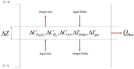
Figure 4.
Schema of control volume around the reduction zone.
Firstly, the extent of the reaction should be defined to derive the balances around the element:
This value for the solid and gas phases has been concluded based on the stochiometric coefficients, mass, and energy balance as follows [13,15]:
where ug is gas velocity, us is solid velocity, and are first and second reaction rate, np is the quantity of pellets per unit of bed volume, is pellet external area, and are gas and solid temperature, is gas molar flow, is heat capacity gas, h is heat transfer coefficient, and is reaction enthalpy.
The aforementioned mathematical modeling of the moving bed direct reduction reactor yields a set of nonlinear ordinary differential equations that can be solved by numerical methods such as Runge–Kutta and the shooting technique [13,15]. Several researchers have made the assumption that, since the radius of the reactor is 200–250 times greater than the pellet diameter, porosity fluctuations of the bed are disregarded [48,49,50,51].
Case Studies
Gilmore, Siderca, Mobarakeh, and Khorasan are industrial units with a comprehensive dataset on network inputs, as shown in Table 3. Using these four industrial units, 200 samples were extracted. Due to insufficient parameters, the dataset of other shaft furnaces could not be used. Developing a new general model using mentioned research dataset from Figure 5 has been considered dimensionless. We employed simulation results from previous research projects as a result of mathematical modeling for feed data. The data in Table 3, in which the error value of mathematical modeling is provided from previous research efforts (Relative Error).
Figure 5.
Different parameters in shaft furnaces at different plants.
The following variables have been selected as network input parameters based on the effective parameters such as dependent and independent in direct reduction simulation to achieve the percentage of X3:
(i) dimensionless temperature of the gas and solid, (ii) percentage of gas entering the furnace, (iii) length-to-diameter ratio of the furnace. The network output is also investigated as a percentage of X3, which is practical for the calculation of the degree of metallization (MD) shown in Equation (13) as a key output parameter [30].
.
Table 3.
Model parameters range for the current study.
Table 3.
Model parameters range for the current study.
| Shaft Furnace Name | (−) | (−) | (−) | (−) | (−) | (−) | (−) | (−) | (−) | (%) | Ref. |
|---|---|---|---|---|---|---|---|---|---|---|---|
| Gilmore | 0–2.2887 | 0.5268–0.37 | 0.2997–0.189 | 0.0465–0.212 | 0.048–0.143 | 0.71–1.08 | 0.33–1.15 | 9589.24 | 93 | 0.215 | [13] |
| Siderca | 0–2.0491 | 0.529–0.49 | 0.347–0.236 | 0.0517–0.124 | 0.0247–0.213 | 0.8–1.01 | 0.36–1.04 | 6580 | 93.7 | 0.106 | [13] |
| Mobarakeh | 0–1.6545 | 0.5357–3292 | 0.3425–2332 | 0.0583–0.2638 | 0.021–0.1373 | 0.7–1.04 | 0.32–1.09 | 7570.41 | 94.8 | 0.949 | [15] |
| Khorasan | 0–1.7857 | 0.53–0.4 | 0.345–0.197 | 0.048–0.180 | 0.022–0.171 | 0.52–1.08 | 0.32–1.11 | 6336.36 | 95.86 | 0.469 | [14] |
3. Artificial Neural Network (ANN)
This work aims to examine government machine learning (ML) strategies for addressing existing difficulties in DRI performance. Additionally, the optimization of machine learning (ML) is a promising method that quickly gains attraction in a variety of fields, such as medicine [52] and engineering [53,54,55,56].
Supervised learning is generally the task of machine learning and learning a function that maps input to output data from sample input–output pairs [57]. During the training process, information is added to the network validation, and the result data performs the network testing process. Training for the network is concluded when generalizations have improved. A variety of active functions have been used to determine the best one. Logistics, Relu, and identity were used to obtain the optimal function of the MLP network. During network training, the predicted network error should be maintained to a minimum for each step of the mean square error (MSE) in each iteration in order to determine the precise network parameter values. The MSE, square of the correlation coefficient (), and root mean square error (RMSE) are used as assessment metrics to relate the model outputs to the validation dataset. MSE, RMSE, and are calculated as follows [58,59,60]:
Three types of algorithms, stochastic gradient descent (SGD) Equation (17) [61], adaptive moment estimation (Adam) Equation (18) [62], and Broyden–Fletcher–Goldfarb–Shanno (BFGS) Equation (19) [63], were applied to find the best ANN algorithm which has the lowest MSE, RMSE, and highest R2. The basic concept of the mentioned algorithms is as follows:
where represents the weight factor, represents the position vector, is the learning rate, represents the cost function, and m represents the first moment.
where is the second moment, and is a small scalar that is used to prevent division by zero.
where is Hussein matrix, is step size, and is Direction of search. The flowchart, as shown in Figure 6, is developed to select the best model.
Figure 6.
Flowchart of optimization for the ANN approach to finding the best network.
4. Results and Discussion
Firstly, the MLP network has been constructed by practicing all three optimization techniques and the Relu activation function. The parameters of the algorithms are optimized to achieve the optimal network. In the SGD algorithm, there are three parameters: batch size, learning rate, and momentum. The batch size is the number of training samples used in one iteration. The learning rate is the amount of each iteration’s step while approaching a minimal loss function. The momentum considers the gradient of previous steps rather than depending just on the current step gradient to control the process. The selected algorithm changes the learning rate and batch size to 0.02 and 20, respectively. A high learning rate enables the model to learn more rapidly but at the expense of a less-than-optimal final weight set. A slower learning rate may enable the model to discover a more optimal or even globally optimal combination of weights, but training will take significantly longer. Concerning deep learning, most practitioners set the value of momentum to 0.9. The optimized SGD algorithm parameters are shown in Figure 7.
Figure 7.
Optimization Parameters SGD algorithm. (a) Study the effect of batch size on the MSE. (b) Study the effect of momentum on the MSE (c) Study the effective learning rate on the MSE.
To examine the RBF network and compare it with the MLP network, RBF network parameters should be optimized. Therefore, according to Figure 8, the spread parameter should be optimized by network data.
Figure 8.
Optimization Spread parameter in RBF network.
4.1. Comparative Analysis of ANN Models
In order to design the structure of the MLP network, it should be optimized for the effective components of the network. One of the most crucial components is the activation function used in the network. According to Figure 9, different activation functions in the MLP network were evaluated according to the number of hidden layer neurons and were found to be the best activation functions. Although the Relu function provides an unsatisfactory output when the number of neurons is smaller than 20, it makes fewer errors when the number of neurons is greater than 20.
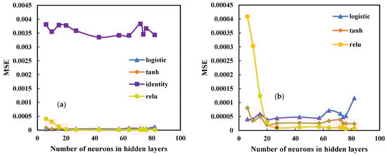
Figure 9.
Comparison between different activation functions to find best function in MLP network (a) comparison of four activation functions; (b) comparison of three activation function.
The MSE, RMSE, and R parameters for the MLP and RBF networks were determined in Table 4 and Table 5. The LBFGS approach is preferable based on the evaluator parameters. In the MLP network, several activation functions and optimization algorithms were also evaluated. As illustrated in Figure 9, the Relu activation function provided a more accurate result.
Figure 10 presents the R of MLP network data with the Relu activation function and different optimization methods in various hidden layer neurons for each network optimization method, which means that the BFGS approach is desirable.
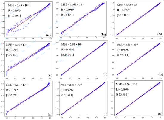
Figure 10.
Comparison accuracy performance of MLP network using the Relu activation function. (a1–a3) SGD method, (b1–b3) Adam method, and (c1–c3) BFGS methods (blue dotes are data and the red line is the fit line).
Table 4.
Accuracy prediction of DRI ANN structures using MLP model algorithms with learning rate = 0.02, momentum = 0.9, and batch size = 20.
Table 4.
Accuracy prediction of DRI ANN structures using MLP model algorithms with learning rate = 0.02, momentum = 0.9, and batch size = 20.
| Optimization Algorithms | Training Function | ||||||||||
|---|---|---|---|---|---|---|---|---|---|---|---|
(−) | (−) | (%) | (%) | Neurons in Hidden Layers | (−) | (−) | (%) | (%) | Neurons in Hidden Layers | ||
| Adam | Relu | 3.05 × 10⁻⁴ | 1.74 × 10⁻² | 0.9985 | 0.9986 | 6 | 8.67 × 10⁻⁵ | 9.3 × 10⁻³ | 0.9995 | 0.9996 | 57 |
| 1.67 × 10⁻⁴ | 1.29 × 10⁻² | 0.9992 | 0.9993 | 10 | 2.48 × 10⁻⁵ | 4.9 × 10⁻³ | 0.9998 | 0.9998 | 64 | ||
| 1.41 × 10⁻⁴ | 1.18 × 10⁻² | 0.9993 | 0.9995 | 15 | 1.77 × 10⁻⁵ | 4.2 × 10⁻³ | 0.9999 | 0.9999 | 72 | ||
| 1.35 × 10⁻⁴ | 1.16 × 10⁻² | 0.9993 | 0.9994 | 20 | 3.76 × 10⁻⁵ | 6.1 × 10⁻³ | 0.9998 | 0.9998 | 74 | ||
| 1.13 × 10⁻⁴ | 1.06 × 10⁻² | 0.9994 | 0.9994 | 27 | 9.61 × 10⁻⁵ | 9.8 × 10⁻³ | 0.9995 | 0.9996 | 76 | ||
| 7.04 × 10⁻⁵ | 8.3 × 10⁻³ | 0.9996 | 0.9997 | 43 | 1.94 × 10⁻⁵ | 4.4 × 10⁻³ | 0.9999 | 0.9999 | 82 | ||
| Broyden, Fletcher, Goldfarb, and Shanno | Relu | 4.09 × 10⁻⁴ | 2.02 × 10⁻² | 0.9980 | 0.9983 | 6 | 1.29 × 10⁻⁵ | 3.6 × 10⁻³ | 0.9999 | 0.9999 | 57 |
| 3.03 × 10⁻⁴ | 1.74 × 10⁻² | 0.9985 | 0.9987 | 10 | 1.7 × 10⁻⁵ | 4.13 × 10⁻³ | 0.9999 | 0.9999 | 64 | ||
| 1.24 × 10⁻⁴ | 1.11 × 10⁻² | 0.9994 | 0.9996 | 15 | 1.05 × 10⁻⁵ | 3.25 × 10⁻³ | 0.9999 | 0.9999 | 72 | ||
| 2.88 × 10⁻⁵ | 5.37 × 10⁻³ | 0.9998 | 0.9998 | 20 | 1.78 × 10⁻⁵ | 4.21 × 10⁻³ | 0.9999 | 0.9999 | 74 | ||
| 8.95 × 10⁻⁶ | 2.99 × 10⁻³ | 0.9999 | 0.9999 | 27 | 5.63 × 10⁻⁶ | 2.37 × 10⁻³ | 0.9999 | 0.9999 | 76 | ||
| 1.15 × 10⁻⁵ | 3.39 × 10⁻³ | 0.9999 | 0.9999 | 43 | 8.15 × 10⁻⁶ | 2.85 × 10⁻³ | 0.9999 | 0.9999 | 82 | ||
| Scaled Conjugate Gradient | Relu | 6.37 × 10⁻³ | 3.94 × 10⁻² | 0.9693 | 0.9695 | 6 | 3.4 × 10⁻⁴ | 1.84 × 10⁻² | 0.9984 | 0.9985 | 57 |
| 5.2 × 10⁻³ | 3.31 × 10⁻² | 0.9734 | 0.9735 | 10 | 1.46 × 10⁻⁴ | 1.21 × 10⁻² | 0.9992 | 0.9992 | 64 | ||
| 2.59 × 10⁻³ | 4.19 × 10⁻² | 0.9877 | 0.9878 | 15 | 3.39 × 10⁻⁴ | 1.84 × 10⁻² | 0.9983 | 0.9984 | 72 | ||
| 9.1 × 10⁻⁴ | 3.02 × 10⁻² | 0.9952 | 0.9955 | 20 | 1.53 × 10⁻⁴ | 1.24 × 10⁻² | 0.9992 | 0.9993 | 74 | ||
| 6.81 × 10⁻⁴ | 2.61 × 10⁻² | 0.9966 | 0.9967 | 27 | 1.38 × 10⁻⁴ | 1.18 × 10⁻² | 0.9993 | 0.9994 | 76 | ||
| 3.9 × 10⁻⁴ | 1.97 × 10⁻² | 0.9981 | 0.9984 | 43 | 2.34 × 10⁻⁴ | 1.53 × 10⁻² | 0.9988 | 0.9990 | 82 | ||
| Broyden, Fletcher, Goldfarb, and Shanno | tanh | 8.08 × 10⁻⁵ | 8.99 × 10⁻³ | 0.9996 | 0.9997 | 6 | 2.59 × 10⁻⁵ | 5.09 × 10⁻³ | 0.9998 | 0.9998 | 57 |
| 3.53 × 10⁻⁵ | 5.94 × 10⁻³ | 0.9998 | 0.9998 | 10 | 3.41 × 10⁻⁵ | 5.84 × 10⁻³ | 0.9998 | 0.9998 | 64 | ||
| 4.86 × 10⁻⁵ | 6.97 × 10⁻³ | 0.9997 | 0.9997 | 15 | 3.82 × 10⁻⁵ | 6.18 × 10⁻³ | 0.9998 | 0.9998 | 72 | ||
| 1.87 × 10⁻⁵ | 4.33 × 10⁻³ | 0.9999 | 0.9999 | 20 | 2.53 × 10⁻⁵ | 5.03 × 10⁻³ | 0.9998 | 0.9998 | 74 | ||
| 2.56 × 10⁻⁵ | 5.06 × 10⁻³ | 0.9998 | 0.9998 | 27 | 2.45 × 10⁻⁵ | 4.95 × 10⁻³ | 0.9998 | 0.9998 | 76 | ||
| 2.69 × 10⁻⁵ | 5.18 × 10⁻³ | 0.9998 | 0.9998 | 43 | 2.39 × 10⁻⁵ | 4.89 × 10⁻³ | 0.9998 | 0.9999 | 82 | ||
| Broyden, Fletcher, Goldfarb, and Shanno | identity | 3.81 × 10⁻³ | 6.17 × 10⁻² | 0.9823 | 0.9825 | 6 | 3.42 × 10⁻³ | 5.85 × 10⁻² | 0.9837 | 0.9839 | 57 |
| 3.55 × 10⁻³ | 5.96 × 10⁻² | 0.9831 | 0.9833 | 10 | 3.41 × 10⁻³ | 5.84 × 10⁻² | 0.9841 | 0.9843 | 64 | ||
| 3.79 × 10⁻³ | 6.15 × 10⁻² | 0.9815 | 0.9818 | 15 | 3.83 × 10⁻³ | 6.19 × 10⁻² | 0.9817 | 0.9817 | 72 | ||
| 3.78 × 10⁻³ | 6.14 × 10⁻² | 0.9828 | 0.9830 | 20 | 3.45 × 10⁻³ | 5.87 × 10⁻² | 0.9835 | 0.9836 | 74 | ||
| 3.58 × 10⁻³ | 5.99 × 10⁻² | 0.9829 | 0.9831 | 27 | 3.67 × 10⁻³ | 6.06 × 10⁻² | 0.9810 | 0.9812 | 76 | ||
| 3.35 × 10⁻³ | 5.79 × 10⁻² | 0.9841 | 0.9844 | 43 | 3.43 × 10⁻³ | 5.86 × 10⁻² | 0.9841 | 0.9842 | 82 | ||
| Broyden, Fletcher, Goldfarb, and Shanno | logistic | 4.05 × 10⁻⁵ | 6.37 × 10⁻³ | 0.9997 | 0.9998 | 6 | 4.54 × 10⁻⁵ | 6.74 × 10⁻³ | 0.9997 | 0.9997 | 57 |
| 4.03 × 10⁻⁵ | 6.35 × 10⁻³ | 0.9998 | 0.9998 | 10 | 7.12 × 10⁻⁵ | 8.44 × 10⁻³ | 0.9996 | 0.9996 | 64 | ||
| 5.92 × 10⁻⁵ | 7.7 × 10⁻³ | 0.9997 | 0.9998 | 15 | 6.02 × 10⁻⁵ | 7.76 × 10⁻³ | 0.9997 | 0.9997 | 72 | ||
| 3.89 × 10⁻⁵ | 6.23 × 10⁻³ | 0.9998 | 0.9998 | 20 | 4.84 × 10⁻⁵ | 6.96 × 10⁻³ | 0.9997 | 0.9997 | 74 | ||
| 4.39 × 10⁻⁵ | 6.62 × 10⁻³ | 0.9997 | 0.9998 | 27 | 5.25 × 10⁻⁵ | 7.25 × 10⁻³ | 0.9997 | 0.9997 | 76 | ||
| 4.8 × 10⁻⁵ | 6.93 × 10⁻³ | 0.9997 | 0.9997 | 43 | 1.16 × 10⁻⁴ | 1.08 × 10⁻² | 0.9994 | 0.9994 | 82 | ||
Table 5.
Accuracy prediction of DRI ANN structures using RBF model algorithms, according to the number of neurons studied and the optimal MLP network.
Table 5.
Accuracy prediction of DRI ANN structures using RBF model algorithms, according to the number of neurons studied and the optimal MLP network.
| Optimization Algorithms | Training Function | (−) | (−) | (%) | (%) | Neurons in Hidden Layers | (−) | (−) | (%) | (%) | Neurons in Hidden Layers |
|---|---|---|---|---|---|---|---|---|---|---|---|
| RBF | Gaussian function | 7.57 × 10⁻³ | 8.7 × 10⁻² | 0.9908 | 0.9908 | 6 | 1.15 × 10⁻⁵ | 3.39 × 10⁻³ | 0.9999 | 0.9999 | 57 |
| 3.66 × 10⁻³ | 6.6 × 10⁻² | 0.9956 | 0.9956 | 10 | 9.8 × 10⁻⁶ | 3.14 × 10⁻³ | 0.9999 | 0.9999 | 64 | ||
| 3.73 × 10⁻⁴ | 1.93 × 10⁻² | 0.9995 | 0.9995 | 15 | 7.8 × 10⁻⁶ | 2.79 × 10⁻³ | 0.9999 | 0.9999 | 72 | ||
| 1.29 × 10⁻⁴ | 1.13 × 10⁻² | 0.9998 | 0.9998 | 20 | 7.6 × 10⁻⁶ | 2.75 × 10⁻³ | 0.9999 | 0.9999 | 74 | ||
| 4.38 × 10⁻⁵ | 6.61 × 10⁻³ | 0.9999 | 0.9999 | 27 | 7.2 × 10⁻⁶ | 2.68 × 10⁻³ | 0.9999 | 0.9999 | 76 | ||
| 1.58 × 10⁻⁵ | 3.97 × 10⁻³ | 0.9999 | 0.9999 | 43 | 6.3 × 10⁻⁶ | 2.5 × 10⁻³ | 0.9999 | 0.9999 | 82 |
As shown in Table 4, the BFGS optimization algorithm method was selected as the optimization method because it has the lowest error considering the number of hidden layer neurons. According to network comparison, the MLP network with the 27 neurons in the hidden layer has the best result and an MSE value of 8.95 × 10⁻⁶. The structures of other networks can cause minor errors when they have more neurons. In Figure 11, three types of different optimization algorithms that have been used for the mlp network are compared with the RBF network. The comparison of different algorithms in Figure 11 shows that the lowest number of neurons concerning the mean squared of error has the LBFG optimization method.
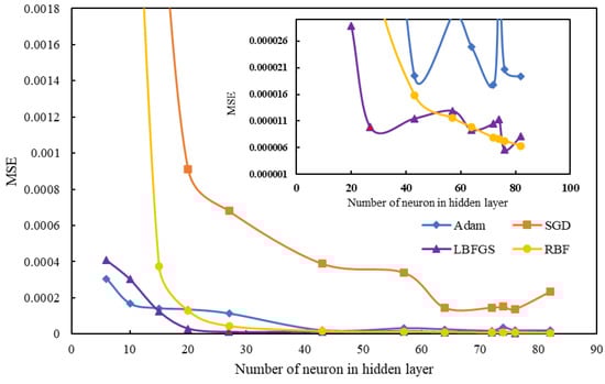
Figure 11.
Comparison of the MLP and RBF networks performance optimization.
4.2. Optimum ANN Results for Prediction of Solid Conversion for DRI Process
The accuracy of network results and the comparison of real data with the prediction amount are quite acceptable. The neural network has a low error rate, and it can calculate the percentage of X3 from the shaft furnace based on input variables such as diameter, length, and input flow to the shaft furnace. The best result was shown using the LBFGS optimization method and the Relu activation function in Figure 12.
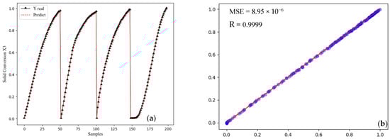
Figure 12.
The best network-developed MLP with two hidden layers (a) Compare predicted using real data (b) strong positive correlation.
As a result, the most functional network consists of two hidden layers, with 13 neurons in the first layer and 14 neurons in the second layer. According to Figure 13, these neurons are fully connected using weights. Furthermore, each neuron has a bias that is listed in Appendix A, along with its weight. The matrix created using the MLP algorithm simulated for the prediction of the MIDREX process is shown in Appendix A.
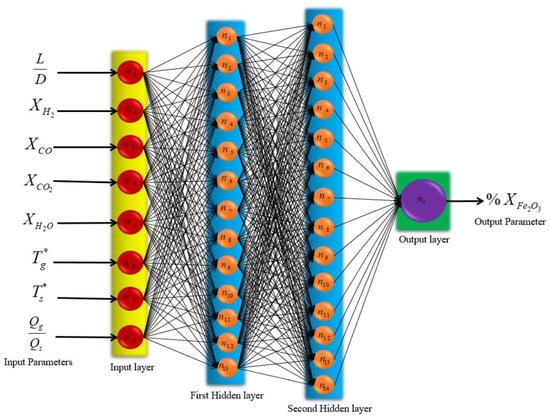
Figure 13.
Schematic of final MLP structure.
4.2.1. Effect of Dimensions on Pellet Conversion Rate
Heatmap and pair plot have been used to show the effects of different parameters on the sponge iron produced, as shown in Figure 14 and Figure 15. In the heatmap chart, Pearson’s correlation coefficients show the relationship between various parameters [64]. In Figure 14, the effect of different parameters of the network is shown as a linear and nonlinear spectrum, with the interpretation that the farther from the unit value (1 and −1), the more nonlinear it is, and the closer to the unit value, the effect of two parameters is proportional and are more linear. The closer value is to one, the more linear relationship between the two parameters. If this value is positive, it indicates a direct relationship between those the two parameters, while if this value is negative, it means that those two parameters are opposite of each other (they increase or decrease in opposite directions). According to Figure 14, the correlation coefficients between the real data of the network and the prediction value of the network are equal to one, which shows that it can completely predict the real data. The correlation coefficient for the effect of dimensions on the conversion rate is 0.91, which shows that the relationship between the two is linear and direct. Based on Figure 15, the direct relationship between these parameters and the degree of linearity is clear. This direct relationship is because of the longer reactor, the longer pellets in the regeneration zone, and the higher conversion rate [15].
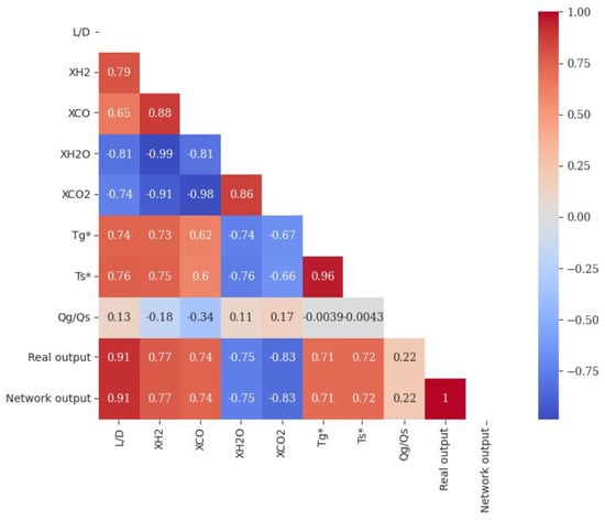
Figure 14.
Heatmap of Pearson correlation coefficient matrix for network MLP.
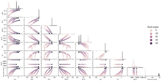
Figure 15.
Comparing the effects of different parameters on each other and on the amount of solid conversion (based on dimensionless data).
4.2.2. The Effect of Gaseous Compounds on Pellet Conversion
According to Figure 14, the correlation coefficient between XCO2 and XH2O with pellet conversion rate is −0.83 and −075, indicating that there is a nonlinear link between them and the direction of their changes is the opposite of each other. These values for the relationship between XCO and XH2 with pellet conversion are equal to 0.74 and 0.77, which proves that the relationship between them is direct and nonlinear. The connection is formed when H2 and CO gases enter the furnace from the bottom of the reduction zone. After interaction with the iron oxide pellets, they turn into CO2 and H2O and exit from the top of the reduction zone. Hence, changes in XCO2 and XH2O have an inverse relationship with changes in pellet conversion rate. From the top of the regeneration zone to the bottom, the amount of pellet conversion increases, and the amount of XCO2 and XH2O decreases. This relationship can be seen in the performance of all stimulations shown in Figure 15 for four shaft furnaces.
4.2.3. The Effect of Flow Rate on Pellet Conversion Rate
According to Figure 14, the correlation coefficient between the ratio of gas to solid flow rate is 0.22. This value proves several facts: firstly, the relationship between the solid flow rate and the pellet conversion rate is opposite of each other because the solid flow rate is in the denominator of the dimensionless flow parameter; secondly, the relationship between the gas flow rate and the conversion rate is because the gas flow rate in the case of the dimensionless flow parameter is direct. In addition, this relationship is nonlinear since the correlation coefficient is near zero. By examination of other parameters in Figure 14, it can be seen that the most nonlinear parameter is the ratio of flow rates. This sign of nonlinearity demonstrates that the impact of this parameter on iron ore recovery is greater than other parameters. This conclusion has been proved by solving the governing equations of the problem [14].
The relationship between solid flow rate and conversion rate is very similar to the relationship between dimensions and conversion rate (both are due to residence time). Furthermore, because of the lower solid flow rate and lower speed of pellets, the pellets and the regeneration gas are more in contact with each other. Consequently, the conversion rate grows as the residence time of the pellets in the regeneration area increases. Contrary to the relationship between solid flow rate and pellet conversion, the pellet conversion rate increases with increasing gas flow rate. This increase is not due to the reduction of external mass transfer resistance from gas to solid. However, simulations reveal that even at the lowest flow rate, the Sherwood number is sufficiently large to render the mass transfer resistance insignificant [15]. Consequently, as the flow rate increases, so does the concentration of reducing gases in the top portion of the reactor.
4.2.4. The Effect of Temperature on the Pellet Conversion Rate
The lowest part of the reduction zone, where the reduction gas enters, has the highest temperature [4]. Furthermore, in this area, the pellet conversion is maximum, proving that increasing the gas and the solid temperature raises the pellet conversion rate. The correlation coefficient between the gas and solid temperature with the solid conversion rate shows the value of 0.71 and 0.72. These values show the direct and nonlinear relationship between the parameters. The smaller the particle, the higher the mass transfer coefficient, which means the film resistance is lower. Thus, the film resistance is maximized if the larger particle is chosen. To explain, if we can remove this film resistance at speed, all smaller particles can be removed at the same speed as the film resistance [50].
Considering the environmental issues, air pollution has been one of the most challenging issues for humans in recent years. Since 7% of carbon dioxide production is derived from the steel industry [9], it can be modeled in future research. The production of Midrex with green hydrogen was aimed at its feasibility from thermal and economic points of view. Another vital issue is the analysis of energy consumption in the MIDREX unit. Recently Salimi et al. investigated the technical and economic study of energy harvesting from the waste heat of the Midrex process by the Kalina cycle in the process of direct iron reduction [65].
5. Conclusions
In this study, two networks were constructed for the percentage of X3 output parameters from the shaft furnace. Two networks were investigated using different optimization methods. The Adam and LBFGS optimization algorithm methods were faster and more accurate, delivering results for MSEs in order 8.95 × 10⁻⁶. Furthermore, various activation functions were practiced to improve the network by the Relu, which can cause the least error due to the number of hidden layer neurons. After optimization of both networks, RBF and MLP, they were compared with the same number of hidden layer neurons. The MLP network was able to generate 8.95 × 10⁻⁶ errors and better predict the conversion percentage of the pellet as an output parameter. This network could be used to improve the performance of the shaft furnace and make modeling to predict the conversion percentage of iron oxide output of the shaft furnace straightforward. The predictive advantage of the shaft furnace can be determined using the network results, such as weights and biases, in the shortest time and with the highest accuracy. Finally, for a better analysis of the effect of different parameters, using a heat map, it was shown that the coefficient of each of the network inputs can communicate with the output and other input parameters of the network. This research could be the beginning of the utilization of ML in the direct reduction process, which is due to the complex behavior of pellets in the shaft furnace and its complex reactions (six heterogeneous reactions of iron oxide phases, methane reforming reactions, water gas shift reactions, and other side reactions) can help the pellet behavior with high speed and accuracy through ML. This modeling is superior to earlier approaches because it is more precise and quick than earlier numerical methods. Another application for ML is in unit control; for instance, it could be used to optimize the temperature of the bustling gas in the shaft furnace. This alone could make for some very fascinating research in the future. ML could be used in future studies for control purposes, such as the MIDREX process.
Author Contributions
Conceptualization, H.M., M.H. and A.E.; Methodology, H.M., M.H. and F.M.; Software, M.H.; Validation, M.H.; Formal analysis, M.H., H.M. and F.M.; Data curation, M.H.; Writing—original draft, M.H., H.M.; Writing—review & editing, H.M. and F.M.; Supervision, A.E.; Project administration, H.M.; Funding acquisition, A.E. All authors have read and agreed to the published version of the manuscript.
Funding
This research received no external funding.
Conflicts of Interest
The authors declare no conflict of interest.
Nomenclature
| Pellet external area [] | |
| Bias [] | |
| , | The heat capacity of solids and gases [] |
| Reduction zone diameter | |
| Cost function | |
| Nonlinear functions of activation transmission | |
| Function of Gaussian | |
| Function | |
| gas molar flow | |
| heat transfer coefficient [W ] | |
| Reaction enthalpy [] | |
| Approximate of the Hussein matrix | |
| Number of neurons in the hidden layer | |
| Position vector | |
| Reduction zone length | |
| first moment (the mean) | |
| Number of data sets for training | |
| number of pellets per unit volume of the bed | |
| n | Neurons |
| Direction of search | |
| Flow-rate | |
| Reaction rate per pellet [ | |
| , | Correlation coefficient [] |
| Direction vector | |
| Dimensionless temperature [] | |
| Dimensionless gas temperature [] | |
| Dimensionless solid temperature [] | |
| Velocity | |
| Second moment (the uncentered variance) | |
| Factor of weight [] | |
| Weight-related to each hidden neuron [] | |
| Input variable [] | |
| The extent of reaction/extent of reactant conversion for [ | |
| The extent of reaction/extent of reactant conversion for [ | |
| Extent of reaction/extent of reactant conversion for [ | |
| Output vector [] | |
| Target output | |
| Greek symbols | |
| Constants in turbulence models [] | |
| Weight of bias for neuron in layer | |
| The output of neuron from the layer of | |
| Step size | |
| Threshold limit [] | |
| Radial Basis Function (RBF) kernel width [] | |
| Gaussian function distribution [] | |
| Subscripts | |
| Characteristic | |
| Reactive solid () | |
| Gas | |
| Gaseous reactant | |
| Pellet | |
| Solid | |
| Acronyms | |
| ANN | Artificial Neural Networks |
| MSE | Mean Square Error |
| Terminology | |
| Neurons | Neurons are the fundamental components of the vast neural network. |
| Bias | Bias is a constant that allows the model to be optimally fitted to the available data. |
| Activation function | This function is a mathematical function between the input that feeds the current neuron and its output that travels to the next layer. |
| Weight | demonstrates the significance and ability of the characteristic/input to the neurons. |
| Epoch | In the training process, each training step’s inputs produce an output that is compared to the goal in order to determine an error. Weights and biases are calculated and adjusted in each epoch using this method. |
| Batch size | For stochastic optimizers, the size of mini-batches is important. (The classifier will not use minibatch if the solver is lbfgs.) |
| Momentum | Update on gradient descending momentum. Only when the solver is sgd. |
| Learning rate | For weight updates, we have to learn a rate schedule (used for SGD). |
Appendix A
Table A1.
Characteristic weights and biases of the model with the best algorithm.
Table A1.
Characteristic weights and biases of the model with the best algorithm.
| Neuron | 1 | 2 | 3 | 4 | 5 | 6 | 7 | 8 | 9 | 10 | 11 | 12 | 13 | 14 | 15 | |
|---|---|---|---|---|---|---|---|---|---|---|---|---|---|---|---|---|
| First hidden layer | −0.5261 | 0.3122 | 0.3003 | −0.3842 | −0.1168 | −0.4217 | −0.4679 | 0.5963 | −0.5029 | 0.2167 | 0.1923 | 0.2747 | −0.0355 | - | - | |
| 0.1414 | −0.6600 | 0.3918 | −0.4975 | −0.1184 | −0.0795 | −0.2839 | 0.2968 | −0.1454 | −0.3495 | 0.1552 | 0.2744 | −0.5067 | ||||
| −0.4716 | 0.1534 | 0.1572 | 0.0499 | −0.1170 | −0.5092 | 0.0669 | 0.3481 | 0.3992 | −0.3800 | −0.0519 | 0.2840 | 0.3226 | - | - | ||
| −0.4195 | 0.2306 | 0.4402 | 0.3055 | −0.3375 | −0.2342 | 0.4835 | 0.5569 | −0.0585 | −0.0243 | 0.3713 | 0.2479 | −0.4035 | - | - | ||
| −0.3103 | −0.4300 | −0.4428 | −0.3570 | −0.1607 | −0.3180 | 0.3841 | 0.3178 | 0.4336 | 0.2486 | −0.0613 | −0.1156 | 0.1871 | - | - | ||
| 0.1264 | 0.2072 | −0.1894 | 0.3279 | −0.4434 | −0.3503 | 0.2591 | −0.1250 | −0.0045 | −0.2883 | −0.1393 | 0.5487 | 0.1746 | - | - | ||
| −0.0399 | 0.4145 | −0.1454 | 0.4606 | 0.4224 | −0.4450 | 0.4078 | 0.1576 | −0.2562 | −0.3226 | −0.4084 | 0.4207 | −0.4346 | - | - | ||
| −0.2834 | 0.6741 | −0.3418 | 0.3441 | 0.1340 | 0.1127 | −0.0791 | −0.1540 | −0.3525 | −0.2026 | −0.2172 | −0.3762 | −0.0161 | - | - | ||
| −0.1834 | −0.1580 | −0.0837 | −0.2541 | 0.1330 | 0.4629 | −0.1553 | −0.2419 | −0.4652 | −0.1960 | −0.3441 | −0.1922 | −0.1461 | - | - | ||
| Second hidden layer | 0.0312 | 0.0689 | 0.4262 | 0.2687 | −0.0318 | 0.1865 | −0.2655 | −0.0196 | 0.1368 | −0.3179 | −0.3118 | −0.0888 | −0.2162 | 0.3304 | - | |
| 0.0045 | 0.2990 | −0.0313 | 0.3231 | 0.0983 | 0.2352 | 0.2577 | 0.3021 | −0.5072 | 0.3468 | −0.0712 | −0.6618 | 0.0328 | 0.3322 | - | ||
| −0.1573 | 0.1815 | 0.1161 | −0.0604 | 0.0848 | −0.4078 | 0.2779 | 0.1774 | −0.1519 | −0.2078 | −0.4528 | −0.3158 | 0.3392 | −0.0341 | - | ||
| 0.5107 | 0.2276 | −0.0847 | 0.3726 | −0.4047 | 0.0170 | 0.2782 | −0.3967 | 0.0856 | 0.2555 | −0.0656 | 0.1127 | −0.0742 | −0.1451 | - | ||
| −0.0711 | −0.4243 | 0.4544 | 0.4096 | 0.1945 | 0.2685 | −0.1691 | 0.2535 | 0.1275 | −0.1207 | 0.0698 | 0.2671 | −0.0571 | 0.3847 | - | ||
| 0.4588 | −0.1143 | 0.1844 | 0.4392 | 0.0310 | 0.0494 | 0.2749 | −0.2550 | −0.3050 | 0.2182 | −0.1881 | −0.0108 | −0.3532 | 0.3005 | - | ||
| 0.2885 | 0.2154 | 0.1225 | 0.0524 | 0.3704 | −0.3282 | 0.3586 | −0.4109 | 0.3636 | −0.3674 | −0.0109 | −0.2198 | 0.3213 | 0.4504 | - | ||
| −0.0564 | 0.2155 | −0.1700 | −0.1756 | −0.0896 | −0.1456 | 0.1221 | −0.1117 | −0.3548 | −0.1415 | 0.1060 | −0.0106 | 0.2727 | −0.5645 | - | ||
| 0.0639 | −0.1984 | −0.1939 | 0.3111 | −0.3191 | −0.3805 | 0.2158 | 0.0610 | −0.2565 | 0.2141 | 0.4456 | −0.2957 | −0.0531 | −0.1954 | - | ||
| −0.2476 | 0.0253 | −0.0674 | −0.0173 | −0.4643 | 0.1050 | 0.1627 | −0.4444 | −0.3693 | 0.3759 | −0.2169 | 0.2445 | 0.3126 | 0.1138 | - | ||
| −0.2510 | 0.3462 | −0.4332 | 0.3669 | −0.4641 | 0.3092 | 0.4015 | 0.0386 | 0.0139 | 0.2427 | −0.3794 | −0.1944 | −0.2762 | −0.1957 | - | ||
| 0.34032 | 0.1627 | −0.0866 | 0.4185 | −0.2898 | −0.3095 | 0.2176 | 0.1026 | 0.1285 | 0.4677 | 0.24473 | 0.0041 | 0.14404 | 0.0999 | - | ||
| −0.4088 | 0.1685 | −0.1742 | 0.4011 | −0.0112 | 0.4490 | 0.1211 | −0.1369 | −0.0108 | 0.2971 | −0.2613 | 0.4224 | 0.2733 | −0.1892 | - | ||
| 0.0027 | 0.3390 | −0.1864 | −0.3606 | −0.3528 | −0.0716 | 0.2954 | −0.3802 | 0.2887 | 0.0372 | 0.3559 | 0.3273 | 0.0601 | 0.2710 | - | ||
| Output layer | 0.1855 | |||||||||||||||
| 0.5334 | ||||||||||||||||
| −0.1828 | ||||||||||||||||
| 0.1919 | ||||||||||||||||
| 0.2326 | ||||||||||||||||
| −0.3029 | ||||||||||||||||
| −0.0028 | ||||||||||||||||
| −0.2619 | ||||||||||||||||
| −0.6629 | ||||||||||||||||
| 0.0341 | - | - | - | - | - | - | - | - | - | - | - | - | - | - | ||
References
- Berg, K.; Olsen, S. Kinetics of manganese ore reduction by carbon monoxide. Metall. Mater. Trans. B 2000, 31, 477–490. [Google Scholar] [CrossRef]
- Szekely, J.; Lin, C.; Sohn, H. A structural model for gas—Solid reactions with a moving boundary—V an experimental study of the reduction of porous nickel-oxide pellets with hydrogen. Chem. Eng. Sci. 1973, 28, 1975–1989. [Google Scholar] [CrossRef]
- Béchara, R.; Hamadeh, H.; Mirgaux, O.; Patisson, F. Carbon impact mitigation of the iron ore direct reduction process through computer-aided optimization and design changes. Metals 2020, 10, 367. [Google Scholar] [CrossRef]
- Hamadeh, H.; Mirgaux, O.; Patisson, F. Detailed modeling of the direct reduction of iron ore in a shaft furnace. Materials 2018, 11, 1865. [Google Scholar] [CrossRef]
- Cavaliere, P. Clean ironmaking and steelmaking processes: Efficient technologies for greenhouse emissions abatement. In Clean Ironmaking and Steelmaking Processes; Springer: Berlin/Heidelberg, Germany, 2019; pp. 1–37. [Google Scholar]
- Cavaliere, P.; Perrone, A.; Silvello, A.; Stagnoli, P.; Duarte, P. Integration of Open Slag Bath Furnace with Direct Reduction Reactors for New-Generation Steelmaking. Metals 2022, 12, 203. [Google Scholar] [CrossRef]
- Statistics, W.D.R. Midrex the World Leader in Direct Reduction Technology; © 2021 Midrex Technologies, Inc.: Charlotte, NC, USA, 2020; pp. 1–15. [Google Scholar]
- Rechberger, K.; Spanlang, A.; Sasiain Conde, A.; Wolfmeir, H.; Harris, C. Green hydrogen-based direct reduction for low-carbon steelmaking. Steel Res. Int. 2020, 91, 2000110. [Google Scholar] [CrossRef]
- Pimm, A.J.; Cockerill, T.T.; Gale, W.F. Energy system requirements of fossil-free steelmaking using hydrogen direct reduction. J. Clean. Prod. 2021, 312, 127665. [Google Scholar] [CrossRef]
- Szekely, J.; El-Tawil, Y. The reduction of hematite pellets with carbon monoxide-hydrogen mixtures. Metall. Trans. B 1976, 7, 490–492. [Google Scholar] [CrossRef]
- Towhidi, N. Reduction kinetics of commercial low-silica hematite pellets with CO-H_2 mixtures over temperature range 600–1234 °C. Ironmak. Steelmak. 1981, 6, 237–249. [Google Scholar]
- Turkdogan, E.; Vinters, J. Gaseous reduction of iron oxides: Part I. Reduction of hematite in hydrogen. Metall. Mater. Trans. B 1971, 2, 3175–3188. [Google Scholar] [CrossRef]
- Parisi, D.R.; Laborde, M.A. Modeling of counter current moving bed gas-solid reactor used in direct reduction of iron ore. Chem. Eng. J. 2004, 104, 35–43. [Google Scholar] [CrossRef]
- Mirzajani, A.; Ebrahim, H.; Nouri, S. Simulation of a direct reduction moving bed reactor using a three interface model. Braz. J. Chem. Eng. 2018, 35, 1019–1028. [Google Scholar] [CrossRef]
- Nouri, S.; Ebrahim, H.A.; Jamshidi, E. Simulation of direct reduction reactor by the grain model. Chem. Eng. J. 2011, 166, 704–709. [Google Scholar] [CrossRef]
- Kazemi, M.; Pour, M.S.; Sichen, D. Experimental and modeling study on reduction of hematite pellets by hydrogen gas. Metall. Mater. Trans. B 2017, 48, 1114–1122. [Google Scholar] [CrossRef]
- McKewan, W. Reduction kinetics of hematite in hydrogen-water vapor-nitrogen mixtures. Trans. Metal Soc. AIME 1962, 224, 2–5. [Google Scholar]
- Usui, T.; Ohmi, M.; Yamamura, E. Analysis of rate of hydrogen reduction of porous wustite pellets basing on zone-reaction models. ISIJ Int. 1990, 30, 347–355. [Google Scholar] [CrossRef]
- Mondal, K.; Lorethova, H.; Hippo, E.; Wiltowski, T.; Lalvani, S. Reduction of iron oxide in carbon monoxide atmosphere—Reaction controlled kinetics. Fuel Process. Technol. 2004, 86, 33–47. [Google Scholar] [CrossRef]
- Tien, R.; Turkdogan, E. Gaseous reduction of iron oxides: Part IV. Mathematical analysis of partial internal reduction-diffusion control. Metall. Trans. 1972, 3, 2039–2048. [Google Scholar] [CrossRef]
- Kam, E. A Model for the Direct Reduction of Iron Ore by Mixtures of Hydrogen and Carbon Monoxide in a Moving Bed; Pascal and Francis: Lawrence, KS, USA, 1981. [Google Scholar]
- Negri, E.D.; Alfano, O.M.; Chiovetta, M.G. Direct reduction of hematite in a moving-bed reactor. Analysis of the water gas shift reaction effects on the reactor behavior. Ind. Eng. Chem. Res. 1991, 30, 474–482. [Google Scholar] [CrossRef]
- Abualigah, L.; Abu Zitar, R.; Almotairi, K.H.; Hussein, A.M.; Elaziz, M.A.; Nikoo, M.R.; Gandomi, A.H. Wind, solar, and photovoltaic renewable energy systems with and without energy storage optimization: A survey of advanced machine learning and deep learning techniques. Energies 2022, 15, 578. [Google Scholar] [CrossRef]
- Said, Z.; Sharma, P.; Aslfattahi, N.; Ghodbane, M. Experimental analysis of novel ionic liquid-MXene hybrid nanofluid’s energy storage properties: Model-prediction using modern ensemble machine learning methods. J. Energy Storage 2022, 52, 104858. [Google Scholar] [CrossRef]
- Forootan, M.M.; Larki, I.; Zahedi, R.; Ahmadi, A. Machine Learning and Deep Learning in Energy Systems: A Review. Sustainability 2022, 14, 4832. [Google Scholar] [CrossRef]
- Valipour, M.S.; Saboohi, Y. Numerical investigation of nonisothermal reduction of hematite using Syngas: The shaft scale study. Model. Simul. Mater. Sci. Eng. 2007, 15, 487. [Google Scholar] [CrossRef]
- Valipour, M.S.; Saboohi, Y. Modeling of multiple noncatalytic gas–solid reactions in a moving bed of porous pellets based on finite volume method. Heat Mass Transf. 2007, 43, 881–894. [Google Scholar] [CrossRef]
- Alamsari, B.; Torii, S.; Trianto, A.; Bindar, Y. Heat and mass transfer in reduction zone of sponge iron reactor. Int. Sch. Res. Not. 2011, 2011, 324659. [Google Scholar] [CrossRef]
- Alhumaizi, K.; Ajbar, A.; Soliman, M. Modelling the complex interactions between reformer and reduction furnace in a midrex-based iron plant. Can. J. Chem. Eng. 2012, 90, 1120–1141. [Google Scholar] [CrossRef]
- Shams, A.; Moazeni, F. Modeling and simulation of the MIDREX shaft furnace: Reduction, transition and cooling Zones. JOM 2015, 67, 2681–2689. [Google Scholar] [CrossRef]
- Ghadi, A.Z.; Valipour, M.S.; Biglari, M. CFD simulation of two-phase gas-particle flow in the Midrex shaft furnace: The effect of twin gas injection system on the performance of the reactor. Int. J. Hydrogen Energy 2017, 42, 103–118. [Google Scholar] [CrossRef]
- Béchara, R.; Hamadeh, H.; Mirgaux, O.; Patisson, F. Optimization of the iron ore direct reduction process through multiscale process modeling. Materials 2018, 11, 1094. [Google Scholar] [CrossRef]
- Hara, Y.; Sakawa, M.; Kondo, S.-I. Mathematical model of the shaft furnace for reduction of iron-ore pellet. Tetsu-Hagané 1976, 62, 315–323. [Google Scholar] [CrossRef]
- Szekely, J.; Evans, J. A structural model for gas-solid reactions with a moving boundary-II: The effect of grain size, porosity and temperature on the reaction of porous pellets. Chem. Eng. Sci. 1971, 26, 1901–1913. [Google Scholar] [CrossRef]
- Szekely, J.; Evans, J. A structural model for gas—Solid reactions with a moving boundary. Chem. Eng. Sci. 1970, 25, 1091–1107. [Google Scholar] [CrossRef]
- Takenaka, Y.; Kimura, Y.; Narita, K.; Kaneko, D. Mathematical model of direct reduction shaft furnace and its application to actual operations of a model plant. Comput. Chem. Eng. 1986, 10, 67–75. [Google Scholar] [CrossRef]
- Yanagiya, T.; Yagi, J.; Omori, Y. Reduction of iron oxide pellets in moving bed. Ironmak. Steelmak. 1979, 6, 93–100. [Google Scholar]
- Kang, H.W.; Chung, W.S.; Murayama, T.; Ono, Y. Effect of iron ore shape on gaseous reduction rate. ISIJ Int. 1998, 38, 1194–1200. [Google Scholar] [CrossRef]
- Kang, H.W.; Chung, W.S.; Murayama, T. Effect of iron ore size on kinetics of gaseous reduction. ISIJ Int. 1998, 38, 109–115. [Google Scholar] [CrossRef]
- Bonalde, A.; Henriquez, A.; Manrique, M. Kinetic analysis of the iron oxide reduction using hydrogen-carbon monoxide mixtures as reducing agent. ISIJ Int. 2005, 45, 1255–1260. [Google Scholar] [CrossRef]
- Rahimi, A.; Niksiar, A. A general model for moving-bed reactors with multiple chemical reactions part I: Model formulation. Int. J. Miner. Process. 2013, 124, 58–66. [Google Scholar] [CrossRef]
- Da Costa, A.R.; Wagner, D.; Patisson, F. Modelling a new, low CO2 emissions, hydrogen steelmaking process. J. Clean. Prod. 2013, 46, 27–35. [Google Scholar] [CrossRef]
- Ponugoti, P.V.; Garg, P.; Geddam, S.N.; Nag, S.; Janardhanan, V.M. Kinetics of iron oxide reduction using CO: Experiments and Modeling. Chem. Eng. J. 2022, 434, 134384. [Google Scholar] [CrossRef]
- Tang, Q.; Huang, K. Determining the kinetic rate constants of Fe3O4-to-Fe and FeO-to-Fe reduction by H2. Chem. Eng. J. 2022, 434, 134771. [Google Scholar] [CrossRef]
- Ajbar, A.; Alhumaizi, K.; Soliman, M. Modeling and simulations of a reformer used in direct reduction of iron. Korean J. Chem. Eng. 2011, 28, 2242–2249. [Google Scholar] [CrossRef]
- Parisi, D.R.; Laborde, M.A. Modeling steady-state heterogeneous gas–solid reactors using feedforward neural networks. Comput. Chem. Eng. 2001, 25, 1241–1250. [Google Scholar] [CrossRef]
- Parisi, D.R.; Mariani, M.a.C.; Laborde, M.A. Solving differential equations with unsupervised neural networks. Chem. Eng. Process. Process Intensif. 2003, 42, 715–721. [Google Scholar] [CrossRef]
- Wu, S.; Xu, J.; Yang, S.; Zhou, Q.; Zhang, L. Basic characteristics of the shaft furnace of COREX® smelting reduction process based on iron oxides reduction simulation. ISIJ Int. 2010, 50, 1032–1039. [Google Scholar] [CrossRef]
- Xu, J.; Wu, S.; Kou, M.; Du, K. Numerical analysis of the characteristics inside pre-reduction shaft furnace and its operation parameters optimization by using a three-dimensional full scale mathematical model. ISIJ Int. 2013, 53, 576–582. [Google Scholar] [CrossRef]
- Wu, S.; Xu, J.; Yagi, J.-I.; Guo, X.; Zhang, L. Prediction of pre-reduction shaft furnace with top gas recycling technology aiming to cut down CO2 emission. ISIJ Int. 2011, 51, 1344–1352. [Google Scholar] [CrossRef]
- Nield, D.; Bejan, A. Convection in Porous Media, 5th ed.; Springer: New York, NY, USA, 2016. [Google Scholar]
- Yusufaly, T.I.; Kallis, K.; Simon, A.; Mayadev, J.; Yashar, C.M.; Einck, J.P.; Mell, L.K.; Brown, D.; Scanderbeg, D.; Hild, S.J.; et al. A knowledge-based organ dose prediction tool for brachytherapy treatment planning of patients with cervical cancer. Brachytherapy 2020, 19, 624–634. [Google Scholar] [CrossRef]
- Zhong, S.; Zhang, K.; Bagheri, M.; Burken, J.G.; Gu, A.; Li, B.; Ma, X.; Marrone, B.L.; Ren, Z.J.; Schrier, J.; et al. Machine learning: New ideas and tools in environmental science and engineering. Environ. Sci. Technol. 2021, 55, 12741–12754. [Google Scholar] [CrossRef]
- Lee, J.H.; Shin, J.; Realff, M.J. Machine learning: Overview of the recent progresses and implications for the process systems engineering field. Comput. Chem. Eng. 2018, 114, 111–121. [Google Scholar] [CrossRef]
- Hegde, J.; Rokseth, B. Applications of machine learning methods for engineering risk assessment–A review. Saf. Sci. 2020, 122, 104492. [Google Scholar] [CrossRef]
- Otchere, D.A.; Ganat, T.O.A.; Gholami, R.; Ridha, S. Application of supervised machine learning paradigms in the prediction of petroleum reservoir properties: Comparative analysis of ANN and SVM models. J. Pet. Sci. Eng. 2021, 200, 108182. [Google Scholar] [CrossRef]
- Han, J.; Pei, J.; Kamber, M. Data Mining: Concepts and Techniques Elsevier Science; Elsevier: Amsterdam, The Netherlands, 2011. [Google Scholar]
- Mashhadimoslem, H.; Vafaeinia, M.; Safarzadeh, M.; Ghaemi, A.; Fathalian, F.; Maleki, A. Development of predictive models for activated carbon synthesis from different biomass for CO2 adsorption using artificial neural networks. Ind. Eng. Chem. Res. 2021, 60, 13950–13966. [Google Scholar] [CrossRef]
- Kolbadinejad, S.; Mashhadimoslem, H.; Ghaemi, A.; Bastos-Neto, M. Deep learning analysis of Ar, Xe, Kr, and O2 adsorption on Activated Carbon and Zeolites using ANN approach. Chem. Eng. Process.-Process Intensif. 2022, 170, 108662. [Google Scholar] [CrossRef]
- Mashhadimoslem, H.; Ghaemi, A. Machine learning analysis and prediction of N2, N2O, and O2 adsorption on activated carbon and carbon molecular sieve. Environ. Sci. Pollut. Res. 2022, 1–21. [Google Scholar] [CrossRef]
- Robbins, H.; Monro, S. A stochastic approximation method. Ann. Math. Stat. 1951, 22, 400–407. [Google Scholar] [CrossRef]
- Kingma, D.P.; Ba, J. Adam: A method for stochastic optimization. arXiv 2014, arXiv:1412.6980. [Google Scholar]
- Fletcher, R. Practical Methods of Optimization; John Wiley & Sons: Hoboken, NJ, USA, 2013. [Google Scholar]
- Egghe, L.; Leydesdorff, L. The relation between Pearson’s correlation coefficient r and Salton’s cosine measure. J. Am. Soc. Inf. Sci. Technol. 2009, 60, 1027–1036. [Google Scholar] [CrossRef]
- Salemi, S.; Torabi, M.; Haghparast, A.K. Technoeconomical investigation of energy harvesting from MIDREX® process waste heat using Kalina cycle in direct reduction iron process. Energy 2022, 239, 122322. [Google Scholar] [CrossRef]
Publisher’s Note: MDPI stays neutral with regard to jurisdictional claims in published maps and institutional affiliations. |
© 2022 by the authors. Licensee MDPI, Basel, Switzerland. This article is an open access article distributed under the terms and conditions of the Creative Commons Attribution (CC BY) license (https://creativecommons.org/licenses/by/4.0/).