1. Introduction
Due to the increase in the amount of renewable energy in the electric grid, it is essential to find suitable compact representations that allow prediction of expected power generation. Such compact representations often improve the prediction quality and can be used to save computational resources and time [
1]. The area of research that deals with finding a suitable representation, e.g., through autoencoders, is called representation learning [
2]. An autoencoder, an artificial neural network architecture, consists of an encoder, a bottleneck layer, and a decoder. In the case of an undercomplete autoencoder, an encoder learns a transformation of the original features into a lower-dimensional feature space, e.g., through a bottleneck in the neural network [
3]. The decoder utilizes this latent representation to reconstruct the original features. Although this area of research has existed in the literature on renewable energy for some time, it is mainly concerned with short-term forecasts, which use wind speed measurements to predict the expected wind power in the following minutes and hours [
4,
5,
6,
7].
At the same time, for planning and ensuring the stability of the electric grid, larger forecast horizons, such as day-ahead forecasts between 24 and 47 h into the future are inevitable. Such prediction horizons are possible with predicted features of numerical weather prediction (NWP) models.
Due to the weather’s chaotic and non-linear behavior, these forecast horizons have more substantial forecast errors than smaller horizons. Therefore, finding suitable representations for those horizons is even more essential. The research questions to find an appropriate representation are:
Answering and developing methods for this question is critical, as in practice, an individual autoencoder is often trained for each wind or photovoltaic (PV) park. This training setting is also called single-task learning (STL), where we train one model for each park individually. At the same time, an MTL architecture reduces the required training time and often improves the forecast error. To our knowledge, MTL autoencoders, trained in a semi-supervised setting, have not been considered for day-ahead power forecasts.
Answering this question allows us to consider seasonality within forecasts, e.g., given through the diurnal cycle, which influences the forecast error [
8].
In the literature, the encoder is often fine-tuned completely for predicting power forecasts. However, as we will see later on, this is not always beneficial and depends on, e.g., the architecture of the autoencoder.
To answer those research questions, we combine techniques from unsupervised learning and MTL. We utilize a discriminative STL autoencoder based on a multi-layer perceptron (MLP) and a temporal convolution network (TCN) for learning latent features of the weather, i.e., referred to as AEMLP and AETCN. The TCN model type is recently introduced for time series forecasts in fields such as speech processing, traffic estimation, short-term wind power predictions [
9], and day-ahead wind and PV power forecasts [
10]. We extend both models in an MTL setting and refer to them as AEMLP-MTL and AETCN-MTL. Our experiments consider a generative approach for all variants through a variational autoencoder (VAE). The generative approach learns to represent the (whole) distribution, while the discriminative autoencoders learn the most efficient data encoding to represent the data. Finally, we train the encoder with a forecasting model in a supervised fashion to forecast the expected power and evaluate the different amount of layers to fine-tune the encoder, leading to the following contributions:
Through the proposed MTL autoencoders, we reduce the number of parameters for training by a factor of 38 for PV data and by 202 times for wind data.
At the same time, we improve the reconstruction error by up to 300% for PV and 134 times for wind through the proposed AETCN-MTL architecture.
During our study, to answer Research Question 3, we found that the number of layers to be fine-tuned depends on the model type, e.g., MLP or TCN and the model architecture, e.g., STL or MTL.
Based on the encoder of the proposed AETCN-MTL model, we achieve one of the best results with improvements up to and percent for PV and wind day-ahead power forecasts, respectively.
The remaining article shows the necessity for a systematic analysis of autoencoders in day-ahead forecasts in
Section 2 through the literature review. Afterward, we detail different autoencoder techniques in
Section 3. The following section,
Section 4, summarizes the datasets and challenges for day-ahead power forecasts. In
Section 5, we detail our analysis to answer the identified research questions. Finally, in
Section 6, we revisit our work and propose future work.
2. Related Work
The following section reviews the related work on wind and PV power forecasts using autoencoders. Within the review, we focus on work that utilizes autoencoder in a transfer learning (TL) setting, e.g., to reduce the required training time. Generally, we consider transfer learning as a knowledge transfer between two tasks. Nowadays, most researchers perform knowledge transfer through fine-tuning layers of a deep learning model. Additional work that applies autoencoders for predicting wind speed and solar radiation is summarized in [
11].
The authors of [
12] are one of the first that considered long-tem short memories (LSTMs) for day-ahead PV power forecasts. Therefore, they initially trained a vanilla autoencoder based on day-ahead NWP inputs from 21 parks. Vanilla autoencoder refers to an autoencoder based on an MLP architecture. Afterward, the authors trained an LSTM attached to the encoder of the autoencoder for renewable power forecasts.
The authors of [
4] proposed the utilization of a stacked autoencoder for multi-step wind power prediction based on an MLP model. The authors trained a three-layer stacked autoencoder on a single wind park based on historical power measurements. Afterward, adding a final layer to the model and fine-tuning the whole network allowed for the creation of multi-step-ahead prediction. The authors evaluated the results on roughly
weeks of data for a one-hour-ahead prediction.
In [
5], a stacked autoencoder was proposed for wind speed and wind power prediction for horizons up to four hours ahead. Compared to [
4], a recurrent autoencoder allowed for learning of the relations in the time series in [
5]. Again, the whole network was fine-tuned after the pre-training and evaluated on two wind speed prediction experiments and one for predicting the expected wind power generation in Belgium.
The third variant of a stacked autoencoder was presented in [
6] for wind power predictions up to two-hours ahead. A particularly engaging aspect of their approach is that they learn the feature extraction of the stacked autoencoder with the power prediction layer jointly in an end-to-end fashion. At the same time, they considered an MTL approach for multi-output predictions, where the model predicts multiple horizons simultaneously. The results were evaluated on a single wind farm in the United States after fine-tuning the complete network.
While the former articles did not explicitly consider TL techniques, the following articles consider techniques from this field. One of the earliest works trained nine MLP-based autoencoders on a single wind park [
7]. Those autoencoders were adapted to four other wind parks and an ensemble given by a deep belief network that combines each park’s extracted features. The authors made a one-hour ahead prediction by utilizing the previous 24 h NWP data, where they reduced the training time through the fine-tuning process from the source park.
The same leading author randomly selected one out of five parks in [
13]. This park was utilized for training a single MLP autoencoder from a randomly selected park. This autoencoder was adapted for every four months of available training data. Over time, there are various autoencoders acting as feature extractors for intra-day forecast horizons. Features extracted from those autoencoders were selected through mutual information and forecasts were combined through an ensemble to provide the final prediction.
The article closest to ours is [
1]. This article compared traditional feature extraction methods with feature extraction techniques from deep learning. The authors showed that fine-tuning helps improve the forecast error for MLP-based models for day-ahead wind and PV power forecasts on a total of 21 PV and 55 wind parks. However, they did not consider autoencoders based on TCNs. Furthermore, an MTL approach was not considered, nor was a different number of layers to unfreeze in the model.
The authors of [
14] trained a unified autoencoder considering data from wind turbines. This model allowed them to extract homogeneous features of all turbines in a base model. To reduce the training time and problem of vanishing gradient, they adopted a model fn a single turbine to extract heterogeneous features and fine-tune the model for the final prediction. Their work considered two experiments with forecast horizons between 10 and 60 s based on meteorological measurements to predict the expected power generation. In the first experiment, they considered 15 parks as the source and target task, whereas in the second experiment they considered 50 parks as the source and target. The unified approach within the article is similar to our proposed MTL approach. However, they only considered an MLP-based model for short forecast horizons, whereas we are interested in the horizon between 24 and 47 h into the future and TCN architecture.
Finally, the authors of [
15] trained variational autoencoders on source parks and fine-tuned this on a target with limited data. They simultaneously utilized five variational datasets as source models to generate several different latent features. The proposed approach reduced the training time while having excellent forecast errors. However, they only used two wind parks as the source domain and three wind parks as the target domain. At the same time, this article utilizes meteorological measurements in a regression task.
Overall we can summarize that only two articles have considered day-ahead power forecast and only one utilized an MTL approach. Even though various articles have considered fine-tuning an initial representation, to the best of our knowledge, none of the articles have evaluated the different number of layers to fine-tune. Furthermore, those techniques are often considered separately. We aim to close this gap with our article. Finally, the maximum number of considered wind parks in the literature are 55 and 21 PV, whereas we considered 445 wind and 117 PV parks.
3. Method
This section explains the deep learning-based techniques for latent feature extraction and concepts of transfer learning and MTL. Latent feature extraction from input features allows the derivation of valuable latent features for downstream tasks such as classification or regression.
We concentrate on undercomplete autoencoders (
Figure 1), as they allow learning a representation
of the input
, where the number of latent features
is less or equal than the input feature dimension
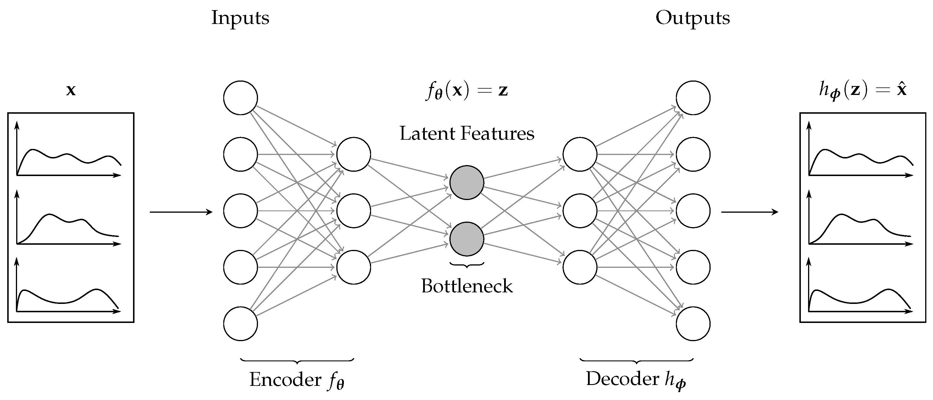
. The concept of undercomplete autoencoders assures that after the training the computational effort is less than with the original input features. Moreover, undercomplete autoencoders are often preferred over overcomplete autoencoders for the same reasons, as they learn a higher dimensional representation of the input features and increase the computational effort in further processing. Within the context of undercomplete autoencoders, we analyze and explain three types of autoencoders:
A combination of those concepts is applicable. For instance, we can train a variational time series autoencoder. Further, we must differentiate if an architecture is learned from single or multiple tasks simultaneously. In the former, we refer to it as an STL and, in the latter case, as an MTL autoencoder.
3.1. Vanilla Autoencoder
Autoencoders describe the concept of learning latent features through neural networks. Within this article, we refer to a vanilla autoencoder as architecture that utilizes an MLP architecture to extract those features. Additionally, we only consider undercomplete autoencoders for reducing the original input features from the NWP, as detailed in
Section 4.1.
In such a vanilla autoencoder, as visualized in
Figure 1, we have three main components: the encoder, the bottleneck, and the decoder. The encoder has the features
from the NWP as input, where the dimension is of size
. In each successive layer, we reduce the number of features to the required number of latent features
, which we refer to as the bottleneck. Afterward, the decoder aims to reconstruct the original features from the latent features
at the bottleneck by increasing the number of features in each successive layer. The difference between the original input and the reconstructed features is referred to as the reconstruction error. We evaluate the reconstruction error often through a squared error loss.
One of the fundamental concepts of autoencoders is the bottleneck. We ensure that the network is not learning an identity mapping during training by having a lower dimension in the bottleneck than in the input. Other alternatives to avoid this problem are, e.g., denoising autoencoders, where we induce random noise on the input features [
1]. However, we excluded those variants as the current results suggest that they are not beneficial over vanilla autoencoders for day-ahead power forecasting [
1].
To introduce the loss function, consider that the latent features are given by the encoder with
, where
is the encoding neural network with parameters
. At the same time, the reconstructed features
and
are given by
, where
is the decoding function given by the neural network with parameters
. In the case that we are interested in reconstruction of the same input features
as output features
, then we aim to approximate the input features with
. We achieve this approximation through the following loss function:
where
L is often a quadratic loss such as the mean squared error (MSE).
After the unsupervised training of an autoencoder through the above loss function, we typically remove the decoder and solely use the learned latent feature as input for supervised machine learning (ML) algorithms for regression or classification tasks. Often, we train this model through a gradient descent method such as the Adam optimizer, where we update the weights of the encoder and those of the forecasting model, e.g., based on a squared error loss.
For results of a squared error loss and a linear decoder, the latent space of the autoencoder lies in a similar sub-space to principal component analysis (PCA). Moreover, ref. [
18] shows that PCA components can be estimated from latent features through singular value decomposition. This result motivates us to utilize PCA as a reference for later experiments.
To compare the predictions obtained with AEs to extended techniques, we extend the idea of AE to more complex structures and further exploit the potential of deep architectures for representation learning in the following.
3.2. Time Series Autoencoder
While a latent representation through an MLP has the advantage that it is easy and efficient to train, this representation neglects cyclic influences, e.g., caused by the diurnal cycle within a day [
8]. Therefore, an autoencoder that learns correlations between timesteps is often beneficial. One choice would be an autoencoder based on a recurrent network such as LSTMs. However, due to the recent success of 1D CNNs for time series forecasts, their reduced training time, and often improved performance, see, e.g., [
17], we focus on these over recurrent architectures. As the principled structure of a time series autoencoder is identical to the vanilla autoencoder detailed in the previous section, we initially focus on the general concept of a one-dimensional convolution autoencoder. Afterward, we detail the proposed TCN autoencoder to learn the latent features from NWP models for day-ahead forecasts.
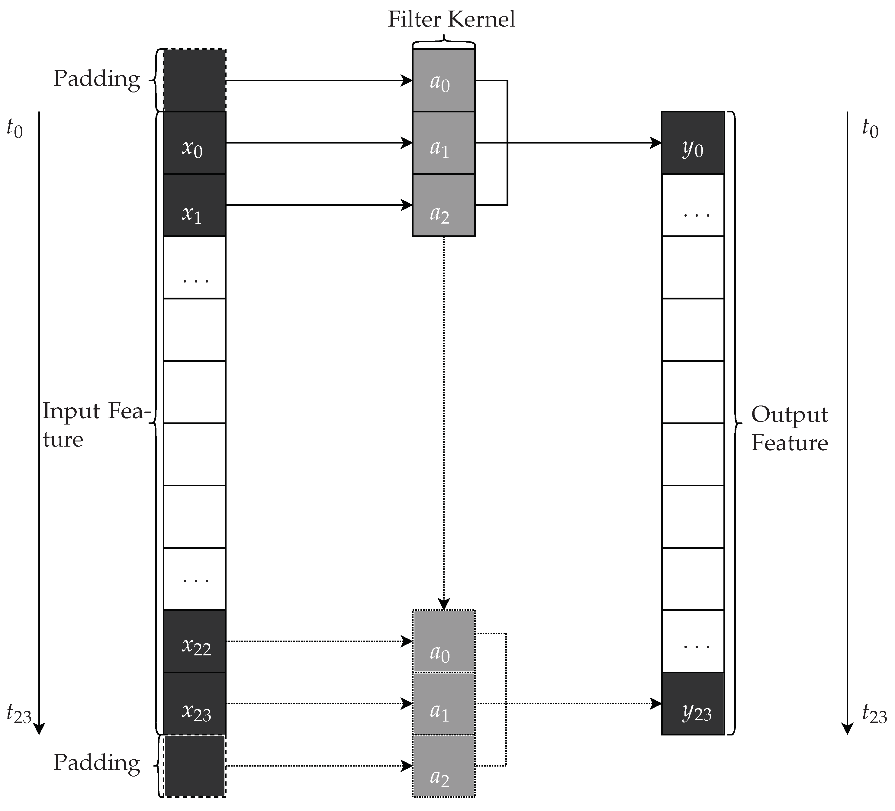
Figure 2 visualizes an example of a 1D-CNN. Let us, therefore, assume we have a one-dimensional input time series with 24 timesteps
t from
similar to the time series length in day-ahead forecasts with an hourly resolution. Let us further assume the time series of a single input feature is given as an ordered set with
, also referred to as input channel, and a filter
. Then, the result of the 1D-CNN at timestep
t is simply given by the dot product between the filter
and
. By adding, e.g., a zero padding at the beginning and end of the time series, we ensure that we maintain the length of the time series, similar to a recurrent network [
19], in the output channel. Padding the time series is also essential, as later on, we aim to forecast the expected power generation with an equivalent time series length.
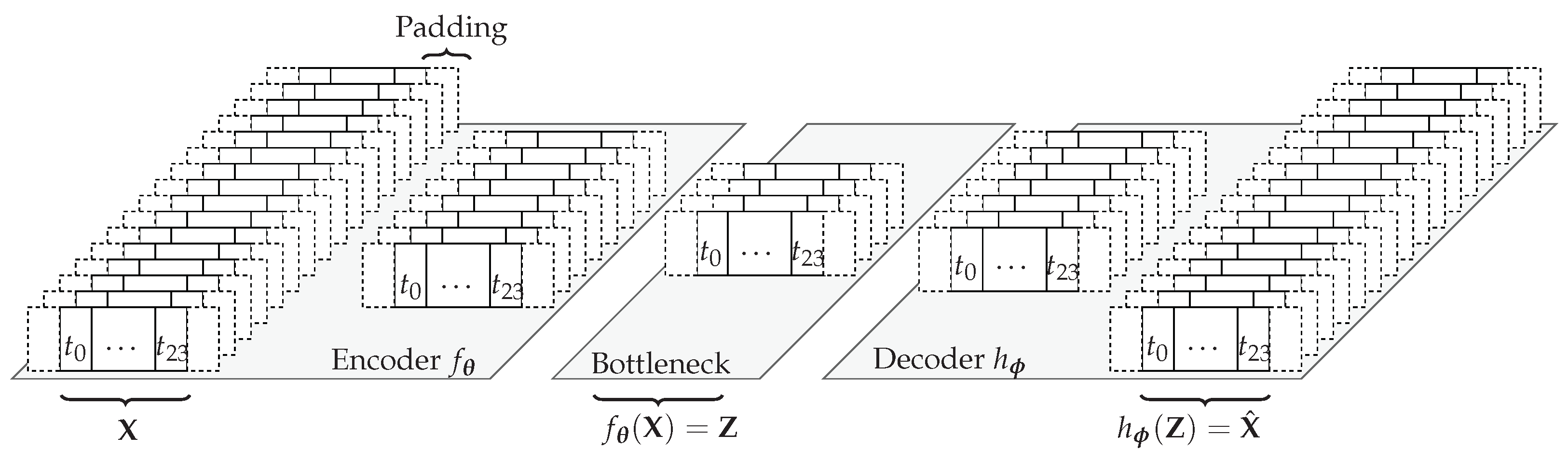
Figure 3 visualizes this concept for multiple inputs. We can observe that in each layer of the encoder, the length of the time series stays the same while the number of features reduces. In the decoder, we increase the number of features. The time series autoencoder now has a tensor
with
as input. Here,
N refers to the number of samples,
is the number of features, and
K is the length of the time series. Again, in our case for day-ahead forecasts, the length of the time series is 24 considering an hourly resolution. The encoder now reduces the dimension to obtain the latent feature tensor
. The decoder approximates the original input tensor with
.
As pointed out earlier, we use the TCN network as the building block for the time series autoencoder. The principle approach is inspired by [
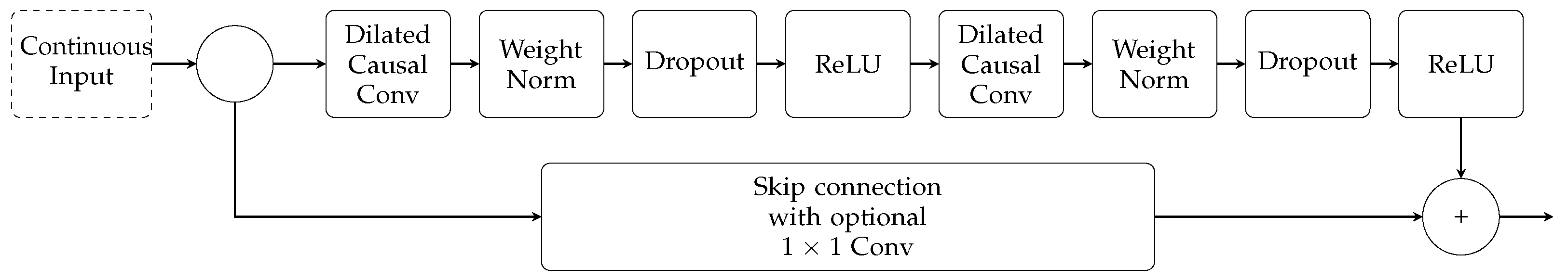
20]. We adapted their proposal to the needs for day-ahead power forecasts. We do not use upsampling or downsampling, as we use zero-padding in all layers and have short time series. As a result, the TCN autoencoder simplifies to a sequential concatenation of residual blocks, as visualized in
Figure 4, of the original TCN network [
21]. The concept of residual blocks is well known in computer vision [
22]. The principle idea behind a residual block is to add a skip connection for the input from previous layers to reduce the risk of the vanishing gradient. Therefore, in each residual block, the input is processed twice in the following pattern: dilated convolution, weight norm, ReLU activation, and dropout for regularization (see
Figure 4). Note that a dilated convolution is a particular convolutional layer that increases the receptive field, is computationally efficient, and requires less memory. The skip connection adds the original input to the output. An optional convolution matches the dimensions in the skip connection if a single layer’s input and output dimensions are unequal.
3.3. Variational Autoencoder
A drawback of the discriminative architectures in the previous sections is that they cannot be used to reconstruct missing values or generate new samples. VAEs are a generative approach that extends the idea of a simple autoencoder by adding a constraint on the encoding site to generative properties.
The encoder
, with parameters
, is forced to learn the mean
and standard deviation
of a Gaussian distribution.
and
are used to create latent features
by sampling from a unit Gaussian translated and are scaled with the learned
and
to obtain
. This is also called the reparameterization trick [
23]. The scaled samples are used to reconstruct the original features
with the decoder
, with parameters
. More formally, this can be done using the loss function:
where the first part, the likelihood function, is equal to the loss function
of an autoencoder (see Equation (
1)). The Kullback–Leibler Divergence
penalizes the deviation between the learned distribution
from a unit Gaussian with
.
By applying the reparameterization trick, it is possible to extend the original idea of an AE and achieve the following properties:
3.4. Transfer Learning
Transfer learning describes the concept of knowledge transfer from one task to another. Knowledge transfer from a source to a target task often has better generalization capabilities and improves the forecast error for problems with limited data. One sub-field of transfer learning is multi-task learning. The term MTL refers to two different concepts: Soft parameter
sharing (SPS) and hard parameter sharing (HPS). The idea that shared knowledge should be used across tasks is included in both principles. However, HPS is advantageous when tasks are closely related and it is advantageous to share a lot of information [
10]. When activities are only slightly related, SPS is helpful, and it is good to have primarily specific knowledge for each task [
10]. When considering a neural network, most layers in the case of HPS are the same for all tasks, and only the final few layers differ. For SPS, we train a single network for each task and regularize the training to make the learned representations of each task similar. Within our work, we consider the extreme case of an HPS autoencoder, where layers of all tasks are the same, as we assume that there is a common latent representation of the weather. While in principle, this might be a simplified consideration, it is the first important step towards finding a common latent representation for forecasting tasks and we can extend the concept to task-specific representation later on, e.g., through task embeddings as proposed in [
10].
Once we learn a joint representation of the weather, we must ensure that the knowledge is appropriate for the target task, in our case, the forecasting of the expected power generation. While an adaption is unnecessary for some latent representations and tasks, this is probably untrue for most. Therefore, we have to adapt knowledge for the task at hand. A common approach in deep learning is the fine-tuning of the final layers of a network. In our case, the encoder extracts the latent features and we adapt the layers of this network. Training an initial network on a source task and adapting it for a target task through fine-tuning is often referenced as sequential transfer learning [
24].
4. Datasets and Challenges in Day-Ahead Power Forecasts
The following sections summarize the datasets and the challenges in day-ahead power forecasts.
4.1. Overall Process of Day-Ahead Forecasts and Challenges
The following section details the challenges associated with day-ahead power forecasts. We include a description of the overall process for generating power forecasts for a wind or PV park.
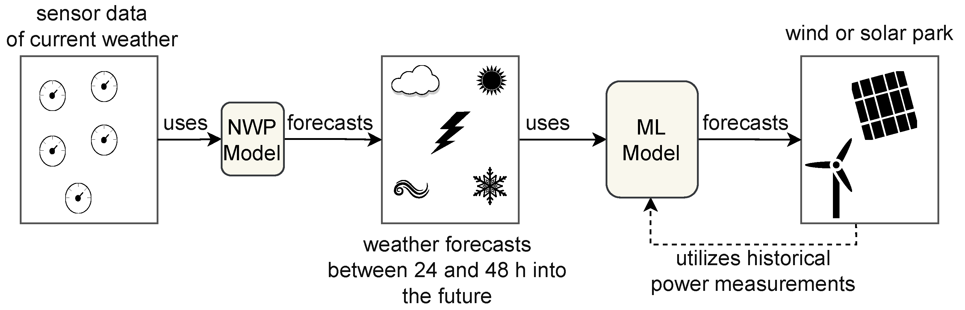
Figure 5 summarizes this process. Due to the weather dependency of renewable power plants, we require weather predictions from so-called NWP models. The NWP model receives input from sensors that approximate the current weather situation. Based on the latest sensory data, a so-called model run is calculated. This model is ran, e.g., at 0.00 a.m. Due to the complex and manifold stochastic differential equations involved in predicting the weather, such a model run typically requires about six hours. Afterward, the NWP provides forecasts, e.g., up to 72 h into the future. In our case, we are interested in so-called day-ahead power forecasts based on weather forecasts between 24 and 47 h into the future. Based on these weather forecasts and historical power measurements, we can train the ML model to predict the expected power generation for day-ahead forecasting problems.
However, due to the dependency of renewable power forecasts on weather forecasts as input features, substantial uncertainty is associated with these forecasts making it a challenging problem. At the same time, weather forecasts are valid for larger grid sizes, e.g., three kilometers, and a mismatch between these grids and the location of a wind or PV causes additional uncertainty in the power forecasts [
25]. These mismatches and the non-linearity of the forecasting problem are depicted in
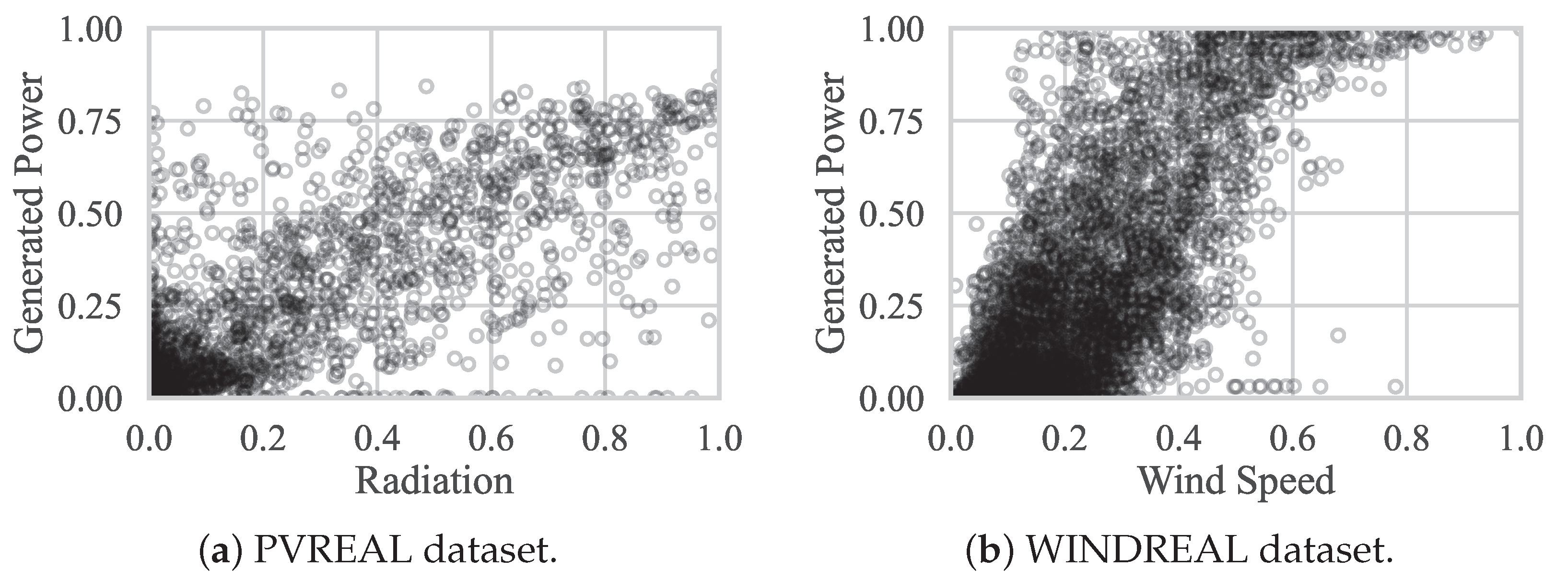
Figure 6. We can observe mismatches between the predicted wind speed (or radiation) and historical power measurements. For instance, we can observe (outliers) where a large amount of power is generated for low values of those features. These mismatches are also shown in the time series plots in
Figure 7. This observation indicates that the weather forecasts were incorrect. While the scatter plot indicates a more linear and straightforward forecasting problem for PV, we can also observe a stronger correlation in the time series than for wind.
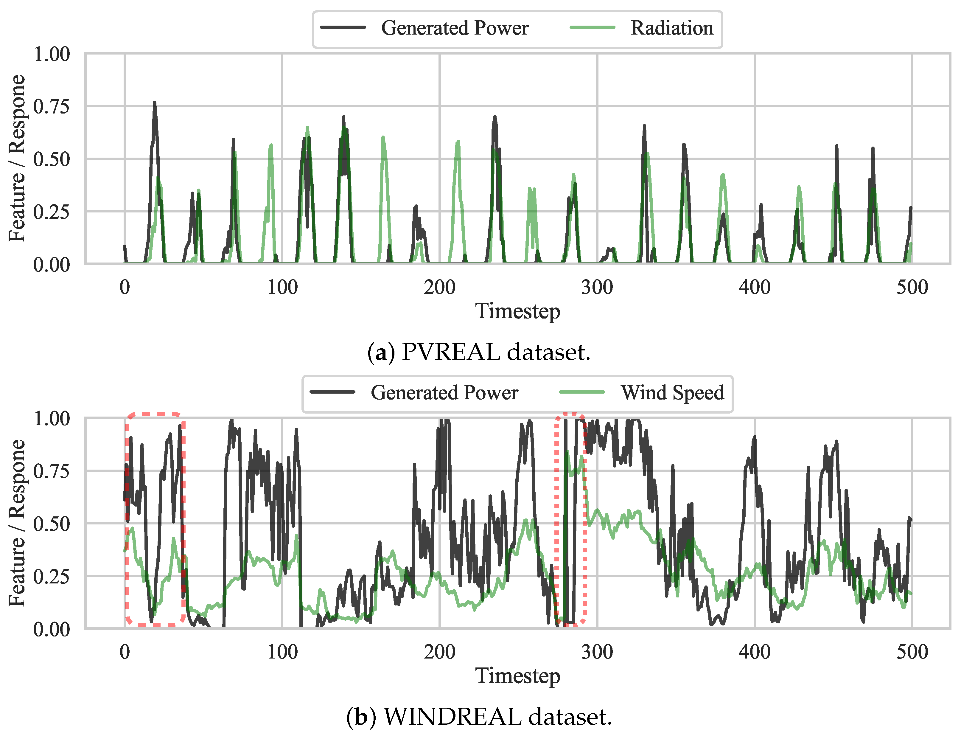
Examples are also present where we observe a considerable amount of wind speed or radiation, but no or little power is generated. An incorrect weather forecast can cause this problem. However, often it is associated with regular interventions. For instance, in some regions in Germany, wind turbines must limit the rotation speed at night. Furthermore, there is a large portion of feed-in management interventions in Germany. These interventions are used to stabilize the electrical grid. A typical pattern for those interventions is given in
Figure 7b at time step 275. We can observe an initial large power production associated with large wind speed values. At this point, the power generation drops to zero while the wind speed remains high. Such a sudden drop is typically associated with feed-in management interventions. As those interventions depend on the power grid’s state, we typically have no information about such drops, making the forecasting problem even more challenging.
4.2. Summary of Datasets
We summarize the considered datasets for learning latent features and predicting the day-ahead power forecasts between 24 and 47 h into the future in
Table 1. The table shows the diversity of the datasets. Each dataset has a different number of parks, input features, training, and test samples. For a better comparison between datasets, we linearly interpolated the PVOPEN datasets from a three-hour to an hourly resolution. All other datasets already had the respective resolution. The datasets also differ in the utilized NWP model. In those weather predictions, from either the European center for medium-range weather forecasts (ECMWF) [
26] or the Icosahedral Nonhydrostatic-European Union (ICON-EU) [
27] weather model, features such as wind speed, wind direction, air pressure, and direct and diffuse radiation are included. For the PVOPEN dataset, various manually engineered features are included, taking seasonal patterns of the sun into account. In the case that a dataset initially did not include seasonal features from the month, day of the year, and hour of the day, we incorporated those through a sine and cosine encoding [
28].
All datasets except the PVREAL and WINDREAL datasets are openly accessible. At the same time, those two datasets are the most recent and diverse. For instance, the WINDREAL dataset includes 13 turbine manufacturers, six hub heights, and 99 different nominal capacities. Furthermore, the PVREAL dataset has various distinct physical characteristics, including ten tilt orientations, 31 different nominal capacities, and nine azimuth orientations. Both datasets include parks located in and around Germany.
The length of these two datasets varies dramatically between parks. Therefore, we considered
randomly sampled days as test data such that we have an equal fraction for training and testing in each park. Note that each day is based on independent day ahead NWP forecasts, so no information is leaked from the future to the past [
25]. This splitting allows for a split without generalization of the test error. For the WINDSYN and PVSYN dataset, on the other hand, the predefined test set is utilized [
30]. Similar to [
29], for the WINDOPEN and PVOPEN, we use the first year’s data as training data and the remaining data as test data. We use
randomly sampled for validation from the training data for all datasets.
5. Experiments
The following sections summarize our results to answer our research questions for the PV and WIND parks from the six datasets. PV parks contain all parks from the datasets PVREAL, PVSYN, and PVOPEN, and WIND refers to all parks from the datasets WINDREAL, WINDSYN, and WINDOPEN.
We first provide details on the overall experimental setup. Afterward, we describe one experiment to evaluate the reconstruction error for the different representation learning techniques for the evaluated latent sizes 2, 4, 6, 8, and 10. The trained autoencoder from this experiment extracting the latent features of the weather (
Figure 8) is then reused for forecasting the expected power in the second experiment described afterward.
5.1. Overall Experimental Setup
For evaluation, we considered the normalized root mean squared error (nRMSE) given by Equation (
4) based on the root mean squared error (RMSE) in Equation (
3). We use Equation (
4) in two ways. First, we utilize it in calculating the reconstruction error to quantify how well a representation learning technique is capable of reconstructing the original features from a latent representation. Secondly, it measures the forecast error for day-ahead power forecasts.
In Equations (
3) and (
4),
is the
i-th value of the response,
is the prediction from a model,
is the number of samples, and
and
are the maximum and minimum values of the response, respectively, a feature. Note that for normalization of the power in all datasets,
is given by the nominal power, whereas for features from the NWP, we consider the empirical minimum and maximum values from the training set.
We considered between two and ten latent features for each experiment. All experiments were conducted on a Slurm cluster and all processes run on one out of four computing nodes, each with 256 AMD EPYC 7742 CPUs and 1008 GB Ram. To answer Research Questions 1 and 2, in the first experiment we evaluated the reconstruction error of the autoencoders. In the second experiment, we evaluated how the encoders from the first experiments can be utilized for power forecasts to answer Research Question 3. In both experiments, we differentiate between WIND and PV parks due to their differences in the expected forecast errors [
8]. The former park type has a total of 490 parks, whereas the latter has 173 parks. For a given park type and the number of latent features, we calculated the mean performance rank based on the nRMSE for both park types. We test for a significant difference compared to the baseline by the Wilcoxon test (
).
5.2. Experiment on Representation Learning for Dimension Reduction
In this section, we answer Research Questions 1 and 2 to evaluate the different representation learning techniques for day-ahead weather forecasts.
5.2.1. Experimental Setup
As a traditional dimension reduction technique we considered a PCA and a kernel PCA with a cosine kernel, referred to as PCA-COSINE. The latter had one of the best results in representation learning for day-ahead power forecasts in [
1]. We compared those two techniques with eight variants of autoencoders as summarized in
Table 2.
Within those autoencoders we either considered an MLP or a TCN model. The former consists of a linear layer followed by the rectified linear unit (ReLU) activation and batchnorm for the input and hidden layers. For the output layers of the encoder and decoder, the activation and batchnorm were not included. The TCN model allows us to take the diurnal behavior of the weather into account and has the structure and non-linear activation functions as described in
Section 3.2.
For each model type, we considered an STL and an MTL approach. For the STL architecture for each park and latent size, we trained an autoencoder. In the case of the MTL architecture, we combined the data of all parks to train a single autoencoder. As all data were combined, we considered this to be a unified AE, where we learn a unified latent space across all parks. It is important to consider here that the MTL architecture has the same number of parameters as the STL approach for a single park. This way, we can evaluate how we can compress features robustly from various parks through a unifying autoencoder.
Within this experiment, the baseline refers to the AEMLP dimension reduction technique. Choosing the AEMLP as baseline allows to compare how MTL architectures improve the reconstruction error for Research Question 1 over STL architectures. Furthermore, it gives insights into how a time series autoencoder improves upon an MLP-based autoencoder for Research Question 2.
The number of input features for autoencoders is equal to that described in
Table 1. Each dataset includes six seasonal features, such as the day of the year, as described in
Section 4.2. These manually engineered features were not included in the output as they are often challenging to learn for autoencoders and we can add those manually. At the same time, including them in the input is essential so that the autoencoder can learn latent features that depend on the seasons. For training, we reduced the number of features in each successive layer by
, up to a minimum of the latent size plus one for all encoder models. The final number of features in the encoder was then equal to the latent size. The decoder had the reverse structure and an additional output layer to map it to the number of features within a park without the seasonal features. For the variational autoencoders, we added one additional layer in the encoder, transforming the latent features into
and
(see
Section 3.3).
To find the best hyperparameters, we conducted a grid search for the learning rate and the number of epochs based on the reconstruction error on the validation dataset. For an STL AE, we selected the best number of epochs from the set along with a learning rate from the set . We initiated five parallel jobs for STL models to train individual parks, where each process had 20 CPUs. While the learning rate was the same, due to the additional data the number of epochs was selected from the set for MTL architectures. For MTL, we trained a model for all parks simultaneously with a single process with 50 CPUs. We trained all MTL deep learning models through the Adam optimizer.
5.2.2. Findings
To show how the required number of parameters is reduced through MTL architectures,
Table 3 provides an overview of the number of parameters for the different models for an example latent size of two. Other latent sizes solely differ slightly in the additional parameters required for the latent features. For both model types, MLP and TCN, when comparing the STL with the MTL architecture, the required number of parameters is reduced 38 times for the PV datasets and 202 times for the wind datasets. The TCN model type, on the other hand, increases the required number of parameters five times over an MLP-based model due to additional parameters in the residual block of the TCN.
We summarize the time consumption of these models in
Table 4. Even though we trained STL models with 100 CPUs through parallelization for each data and model type and the MTL models were trained only with 50 CPUs, we can observe a substantial reduction in the training time. Often the STL models require at least five times more computation time, even though we trained them with additional CPUs. For a few cases, the computation time of MTL is even ten times less than that of an STL architecture.
The mean performance rank results for the reconstruction error of all models are depicted in
Table 5. We summarize the median reconstruction errors based on Equation (
4) in
Table 6. These tables show that the variational autoencoders have the worst results, regardless of the architecture and model type used. The variational autoencoders are significantly worse than the baseline for all latent sizes and the two data types. For instance, for a latent size of ten, the median nRMSE of the baseline is
lower than the best variational autoencoder for the WIND parks. Similarly, for PV parks, the baseline is at least
better than the variational autoencoder. This observation likely occurs due to the limitation of the variational distribution that restricts the latent space through the normal distribution. This effect can potentially be reduced by scaling the Kullback–Leibler divergence in Equation (
2).
Another interesting observation is that the mean performance rank in all cases is larger for variational MTL autoencoders than for the same STL architecture. At the same time, the difference in the median reconstruction error is only about . Again, we can explain this result with the variational distribution. In the case of the MTL architecture, the same variational distribution must express multiple parks. Intuitively enough, as the STL architecture already has difficulties compressing the information in the latent space, it is even more challenging in an MTL setting. As all models share the same number of layers, it might be beneficial for the variational autoencoder to utilize a deeper network or a larger latent size to ease the training. Again, another option would be to reduce the constraint given through the Kullback–Leibler divergence. With the evaluated hyperparameters, we can summarize that the MTL architecture is not beneficial for variational autoencoders.
On the other hand, regarding Research Question 2, the results are different. We can observe that regardless of the architecture, the mean performance rank is better for time series autoencoders for PV parks. For WIND parks, the time series autoencoders are worse than the MLP-based variational autoencoders. These differences in the data types are best explained by the diurnal cycle of a day that influences the forecast for PV parks more than for WIND parks (see [
8]).
We can make similar conclusions for the PCA-COSINE representation technique than for the variational autoencoders. A transformation through a cosine kernel seems too restrictive or unsuitable for the data at hand. On the other hand, the PCA model is, at least for the WIND data type, better than the baseline up to a latent size of four. For PV parks, the PCA is significantly worse except for with a latent size of ten.
As the baseline substantially outperforms the PCA-based models and the variational autoencoders, we can safely assume that the AEMLP is a reliable baseline method. The MTL architecture of the baseline, the AEMLP-MTL model, significantly outperforms this reference in all cases. The improvements in the median nRMSE range from 9 to for WIND parks and between 16 and for PV parks. We also achieve improvements through the MTL architecture for time series autoencoders. The MTL time series autoencoder has the best median performance rank for all latent sizes and data types. Thereby, concerning Research Question 1, we can conclude that we substantially improve the reconstruction error for discriminative autoencoders through an MTL architecture. This result contrasts with the generative autoencoder results, where the MTL architecture worsens the results. However, the discriminative autoencoder is not limited by the variational distribution. Without this limitation, the autoencoder learns a better encoding for the weather features through the MTL approach. The additional training samples from all parks allow us to learn an encoding that generalizes better during test time. The improvements can be best explained by the fact that in an MTL setting, we train with weather conditions from other parks that would otherwise not be available in an STL training. During test time, this allows the network to use knowledge from all parks.
To answer Research Question 2 for discriminative autoencoders we need to differentiate between STL and MTL architectures. While the median nRMSE of the STL time series autoencoder is often of similar magnitude to the baseline, the results are only significantly better or equal in six cases. The critical improvements come in combination with the MTL architecture. As pointed out earlier, this model is the best for all tested latent sizes and data types. For PV parks, the improvements of the median error range from 68– and between 46 and for WIND. Here, we can assume that the STL time series autoencoder differs from the MTL approach, as additional training samples are required for the additional parameters and learning the particular requirements in learning the diurnal cycle. Overall we can summarize the results as follows:
Generative autoencoders need further investigation regarding influences of the latent size, the network structure, and the scaling of the Kullback–Leibler divergence to answer the research questions.
MTL architectures improve the reconstruction error substantially for discriminative autoencoders.
Time series autoencoders significantly improve when combined with an MTL architecture.
5.3. Experiment on Wind and PV Power Forecasts
Within this section, we answer Research Question 3 to evaluate the importance of fine-tuning the encoder for day-ahead power predictions.
5.3.1. Experimental Setup
In the experiment described in this section, we considered the models from
Section 5.2 as models for feature extraction. These models were used to extract the latent features utilized to make predictions for wind and PV day-ahead power forecasts. As forecasting models, we considered an MLP and a TCN attached to the encoder with the same model type from the previous experiment. For the PCA and PCA-COSINE representation learning technique, we also considered an MLP for forecasting the expected power generation. We chose the hidden layers to be 200 and 100 neurons for the MLP. Due to the additional parameters in the residual block of the TCN, the hidden layers were of size 60 and 30. These two forecasting models were trained for ten epochs with cosine annealing with a maximum learning rate of
and afterward with a maximum learning rate of
for another ten epochs with cosine annealing through the Adam optimizer.
The batch size was selected to have ten iterations within each epoch. We evaluated whether it was beneficial to fine-tune the encoder models and we fine-tuned zero, one, or two layers of the encoder models. As in the previous experiment, we utilized the AEMLP for latent feature extraction as a baseline and attached an MLP for forecasting the power. In principle, we could have also attached other models to the encoder, such as a linear model or a gradient boosting regression tree. However, forecast errors for different forecasting models are often in a similar range [
1] and it is difficult to fine-tune the encoder in an end-to-end fashion for those models.
5.3.2. Findings
The results that we use to answer Research Question 3 are summarized in
Table 7 and
Table 8. We only consider those models that are within the two best ranked models for readability. The naming conventions are the same as in the previous section for the dimension reduction techniques. Additionally, we add the considered forecasting model. The results indicate the number of fine-tuned layers that are 1 or 2. For example, AEMLP-MTL-MLP1 depicts the AEMLP-MTL feature extraction technique coupled with the MLP forecasting model and the fine-tuning of the last layer of the encoder.
Compared to the previous experiment, there is no prominent best model. Not surprisingly, none of the variational autoencoder architectures are among the best models, as learned latent features are insufficient for reconstructing the original features. Unlike the previous experiment, PCA and PCA-COSINE now achieve the best results in two cases for PV parks. Except for a latent size of two, the PCA-MLP and the PCA-COSINE-MLP outperform the baseline significantly for this data type. For WIND parks, these models are significantly worse for most latent sizes.
For the AEMLP-MLP model, we can observe that fine-tuning the final layer is at least as good as the baseline (the same model without fine-tuning). Fine-tuning the second last layer of the encoder leads to worse results and is not within the best models. We can assume that due to the STL approach, the latent features are already close to a representation required for forecasting the expected power and only slight adjustments in the encoder are required.
For the STL time series encoder, we need to fine-tune two layers such that the model is among the best and at least as good as the baseline. For the PV parks, improvements up to are present, whereas for WIND, these are at about .
For the MTL variant of the baseline, the AEMLP-MTL-MLP model, we can observe no substantial difference between fine-tuning one or two layers. Nevertheless, the results of this model without fine-tuning are worse than with the adaption of the encoder. Furthermore, in three cases, AEMLP-MTL-MLP1 and AEMLP-MTL-MLP2 are significantly worse than the baseline. These results are engaging in a manifold way. In the previous experiment, we saw that the MTL architecture outperforms the STL approach for representation learning significantly in all cases for the MLP-based autoencoder. This relation is no longer the case for forecasting historical power. We can assume here that, on the one hand, the learned latent space needs to be adapted for forecasting the power in general. On the other hand, due to the MTL approach, the latent space is too broad and careful fine-tuning is needed to adapt the encoder model for the specific requirements of a single park. This problem was not present for the STL architecture, where the forecast errors were always as least as good as the baseline.
The AETCN-MTL-TCN model is consistently among the best for latent sizes up to six. When fine-tuning two layers of the encoder, it is only worse than the baseline in one case. We can also observe, except for this case, that fine-tuning two layers improves the forecast error compared to a single layer. For the PV parks, we achieved improvements between % and for the median forecast error, whereas for WIND parks, we accomplished advances in the error ranging from to . In contrast to the MLP-based MTL autoencoder, we can assume that the fine-tuning of the encoder is more reliable for CNN layers than for MLP layers. Overall the results can be summarized as follows:
For forecasting the day-ahead power generation based on an AE-MLP autoencoder and MLP forecasting model, fine-tuning only the last layer of the encoder for STL architectures leads to the most reliable results.
When considering a time series autoencoder such as the proposed AE-TCN, an MTL approach and the fine-tuning of two layers of the encoder leads to the best and most consistent results regardless of the data type and latent size.
6. Conclusions and Future Work
This article studied autoencoders for day-ahead wind and solar power forecasts. By considering generative, discriminative, vanilla, and time series autoencoders, we considered a broad range of architectures to find the most applicable representation learning technique. We found that multi-task autoencoders improve reconstruction errors for discriminative autoencoders. A combination of multi-task and time series autoencoders led to an almost perfect ranking of the reconstruction error. By considering a multi-task approach, we reduced the trainable parameters by up to 203 times. Finally, we can conclude that the amount of layers to fine-tune depends on the architecture and the model. For single-task learning architectures and a multi-layer perceptron-based autoencoder, fine-tuning a single layer is sufficient. In contrast, for single-task time series, an autoencoder including additional layers is beneficial, whereas for multi-task architectures, it is always beneficial to include multiple layers during fine-tuning.
Due to the restrictions of the variational distribution of variational autoencoders, we could not find a sufficiently good representation. In future work, we will need to extend the analysis for this model concerning the latent size, the number of layers in the network, and the scaling of the Kullback–Leibler divergence.
Author Contributions
Conceptualization, J.S.; methodology, J.S.; software, J.S.; validation, J.S.; formal analysis, J.S.; investigation, J.S.; resources, J.S.; data curation, J.S.; writing—original draft preparation, J.S.; writing—review and editing, J.S.; visualization, J.S.; supervision, B.S.; project administration, J.S.; funding acquisition, B.S. All authors have read and agreed to the published version of the manuscript.
Funding
This work results from the project TRANSFER (01IS20020B) funded by BMBF (German Federal Ministry of Education and Research). Enercast GmbH has provided the real-world datasets.
Data Availability Statement
Acknowledgments
We thank Mohammad Wazed Ali, Diego Botache, Christian Gruhl, Stephan Vogt, and Alyssa Opland for their valuable input and feedback.
Conflicts of Interest
The authors declare no conflict of interest.
References
- Henze, J.; Schreiber, J.; Sick, B. Representation Learning in Power Time Series Forecasting. In Deep Learning: Algorithms and Applications; Springer: Cham, Switzerland, 2020; pp. 67–101. [Google Scholar] [CrossRef]
- Bengio, Y.; Courville, A.; Vincent, P. Representation Learning: A Review and New Perspectives. arXiv 2012, arXiv:1206.5538. [Google Scholar] [CrossRef] [PubMed]
- Goodfellow, I.; Bengio, Y.; Courville, A. Deep Learning; MIT Press: Cambridge, MA, USA, 2016; p. 775. [Google Scholar]
- Jiao, R.; Huang, X.; Ma, X.; Han, L.; Tian, W. A Model Combining Stacked Auto Encoder and Back Propagation Algorithm for Short-Term Wind Power Forecasting. IEEE Access 2018, 6, 17851–17858. [Google Scholar] [CrossRef]
- Wang, L.; Tao, R.; Hu, H.; Zeng, Y.-R. Effective wind power prediction using novel deep learning network: Stacked independently recurrent autoencoder. Renew. Energy 2021, 164, 642–655. [Google Scholar] [CrossRef]
- Chen, J.; Zhu, Q.; Li, H.; Zhu, L.; Shi, D.; Li, Y.; Duan, X.; Liu, Y. Learning Heterogeneous Features Jointly: A Deep End-to-End Framework for Multi-Step Short-Term Wind Power Prediction. IEEE Trans. Sustain. Energy 2020, 11, 1761–1772. [Google Scholar] [CrossRef]
- Qureshi, A.S.; Khan, A.; Zameer, A.; Usman, A. Wind power prediction using deep neural network based meta regression and transfer learning. Appl. Soft Comput. 2017, 58, 742–755. [Google Scholar] [CrossRef]
- Schreiber, J.; Buschin, A.; Sick, B. Influences in Forecast Errors for Wind and Photovoltaic Power: A Study on Machine Learning Models. In INFORMATIK 2019; GI e.V.: Bonn, Germany, 2019; pp. 585–598. [Google Scholar] [CrossRef]
- Zhu, R.; Liao, W.; Wang, Y. Short-term prediction for wind power based on temporal convolutional network. Energy Rep. 2020, 6, 424–429. [Google Scholar] [CrossRef]
- Schreiber, J.; Sick, B. Emerging Relation Network and Task Embedding for Multi-Task Regression Problems. In Proceedings of the ICPR 2020, Milan, Italy, 22–24 September 2020; pp. 2663–2670. [Google Scholar] [CrossRef]
- Alkhayat, G.; Mehmood, R. A review and taxonomy of wind and solar energy forecasting methods based on deep learning. Energy AI 2021, 4, 100060. [Google Scholar] [CrossRef]
- Gensler, A.; Henze, J.; Sick, B.; Raabe, N. Deep Learning for solar power forecasting—An approach using AutoEncoder and LSTM Neural Networks. In Proceedings of the 2016 IEEE International Conference on Systems, Man, and Cybernetics, Budapest, Hungary, 9–12 October 2016; pp. 2858–2865. [Google Scholar]
- Qureshi, A.S.; Khan, A. Adaptive transfer learning in deep neural networks: Wind power prediction using knowledge transfer from region to region and between different task domains. Comput. Intell. 2019, 35, 1088–1112. [Google Scholar] [CrossRef]
- Liu, X.; Cao, Z.; Zhang, Z. Short-term predictions of multiple wind turbine power outputs based on deep neural networks with transfer learning. Energy 2021, 217, 119356. [Google Scholar] [CrossRef]
- Khan, M.; Naeem, M.R.; Al-Ammar, E.A.; Ko, W.; Vettikalladi, H.; Ahmad, I. Power Forecasting of Regional Wind Farms via Variational Auto-Encoder and Deep Hybrid Transfer Learning. Electronics 2022, 11, 206. [Google Scholar] [CrossRef]
- Fawaz, H.I.; Forestier, G.; Weber, J.; Idoumghar, L.; Muller, P.-A. Transfer learning for time series classification. In Proceedings of the 2018 IEEE BigData, Seattle, WA, USA, 10–13 December 2018; pp. 1367–1376. [Google Scholar] [CrossRef]
- Yan, J.; Mu, L.; Wang, L.; Ranjan, R.; Zomaya, A.Y. Temporal Convolutional Networks for the Advance Prediction of ENSO. Sci. Rep. 2020, 10, 8055. [Google Scholar] [CrossRef] [PubMed]
- Plaut, E. From Principal Subspaces to Principal Components with Linear Autoencoders. arXiv 2018, arXiv:1804.10253. [Google Scholar]
- Yan, C.; Pan, Y.; Archer, C.L. A general method to estimate wind farm power using artificial neural networks. Wind Energy 2019, 22, 1421–1432. [Google Scholar] [CrossRef]
- Thill, M.; Konen, W.; Bäck, T. Time Series Encodings with Temporal Convolutional Networks. In BIOMA 2020: Bioinspired Optimization Methods and Their Applications; Lecture Notes in Computer Science (including subseries Lecture Notes in Artificial Intelligence and Lecture Notes in Bioinformatics); Springer: Berlin/Heidelberg, Germany, 2020; Volume 12438, pp. 161–173. [Google Scholar] [CrossRef]
- Lea, C.; Vidal, R.; Reiter, A.; Hager, G.D. Temporal convolutional networks: A unified approach to action segmentation. In Computer Vision—ECCV 2016 Workshops; Springer: Berlin/Heidelberg, Germany, 2016; pp. 47–54. [Google Scholar] [CrossRef]
- He, K.; Zhang, X.; Ren, S.; Sun, J. Deep Residual Learning for Image Recognition. In Proceedings of the IEEE Conference on Computer Vision and Pattern Recognition (CVPR), Las Vegas, NV, USA, 27–30 June 2016; pp. 1–112. [Google Scholar] [CrossRef]
- Kingma, D.P.; Welling, M. Auto-Encoding Variational Bayes. arXiv 2013, arXiv:1312.6114. [Google Scholar]
- Ruder, S. Neural Transfer Learning for Natural Language Processing. Ph.D. Thesis, National University of Ireland, Galway, Ireland, 2019. [Google Scholar]
- Gensler, A. Wind Power Ensemble Forecasting. Ph.D. Thesis, University of Kassel, Kassel, Germany, 2018. [Google Scholar]
- European Centre for Medium-Range Weather Forecasts. 2020. Available online: http://www.ecmwf.int/ (accessed on 24 August 2022).
- Icosahedral Nonhydrostatic-European Union. 2022. Available online: https://www.dwd.de/SharedDocs/downloads/DE/modelldokumentationen/nwv/icon/icon_dbbeschr_aktuell.pdf? (accessed on 24 August 2022).
- Lewinson, E. Three Approaches to Encoding Time Information as Features for ML Models. 2022. Available online: https://developer.nvidia.com/blog/three-approaches-to-encoding-time-information-as-features-for-ml-models/ (accessed on 8 July 2022).
- Schreiber, J.; Vogt, S.; Sick, B. Task Embedding Temporal Convolution Networks for Transfer Learning Problems in Renewable Power Time-Series Forecast. In Proceedings of the ECML, Virtual, 13–17 September 2021; pp. 118–134. [Google Scholar] [CrossRef]
- Vogt, S.; Schreiber, J. Synthetic Photovoltaic and Wind Power Forecasting Data. arXiv 2022, arXiv:2204.00411. [Google Scholar]
- Schreiber, J.; Sick, B. Model Selection, Adaptation, and Combination for Transfer Learning in Wind and Photovoltaic Power Forecasts. arXiv 2022, arXiv:2204.13293. [Google Scholar] [CrossRef]
Figure 1.
An example undercomplete autoencoder (AE) topology. The AE reduces the dimensionality in each layer of the encoder. The representation of the latent features at the bottleneck are the extracted hidden features sufficient to reconstruct the original input successively in each layer of the decoder.
Figure 2.
Example one-dimensional CNN with a filter of size . We keep the time series’ dimension and extract relevant information by applying the filter to an input time series size of with additional padding.
Figure 2.
Example one-dimensional CNN with a filter of size . We keep the time series’ dimension and extract relevant information by applying the filter to an input time series size of with additional padding.
Figure 3.
An example undercomplete time series AE topology. The AE reduces the dimensionality in each layer of the encoder. The latent features’ representation at the bottleneck are the extracted hidden features sufficient to reconstruct the original input successively in each layer of the decoder.
Figure 3.
An example undercomplete time series AE topology. The AE reduces the dimensionality in each layer of the encoder. The latent features’ representation at the bottleneck are the extracted hidden features sufficient to reconstruct the original input successively in each layer of the decoder.
Figure 4.
Residual block of the TCN.
Figure 4.
Residual block of the TCN.
Figure 5.
Overview of renewable power forecast process.
Figure 5.
Overview of renewable power forecast process.
Figure 6.
Scatter plots of the most relevant features for power forecasts from day-ahead weather forecasts and the historical power measurements. Large radiation or wind speed values and no power generation indicate an incorrect weather forecast or feed-in management. Large power generation values and a low value of wind speed or radiation indicate an incorrect weather forecast.
Figure 7.
Time series plots of most relevant features for power forecasts from day-ahead weather forecasts and the historical power measurements. The radiation, as well as the historical power, shows a typical Gaussian-shaped behavior during the day. The dashed rectangle shows a potential bad weather forecast of the wind speed. The dotted rectangle for the WINDREAL dataset indicates a typical pattern of feed-in management interventions.
Figure 8.
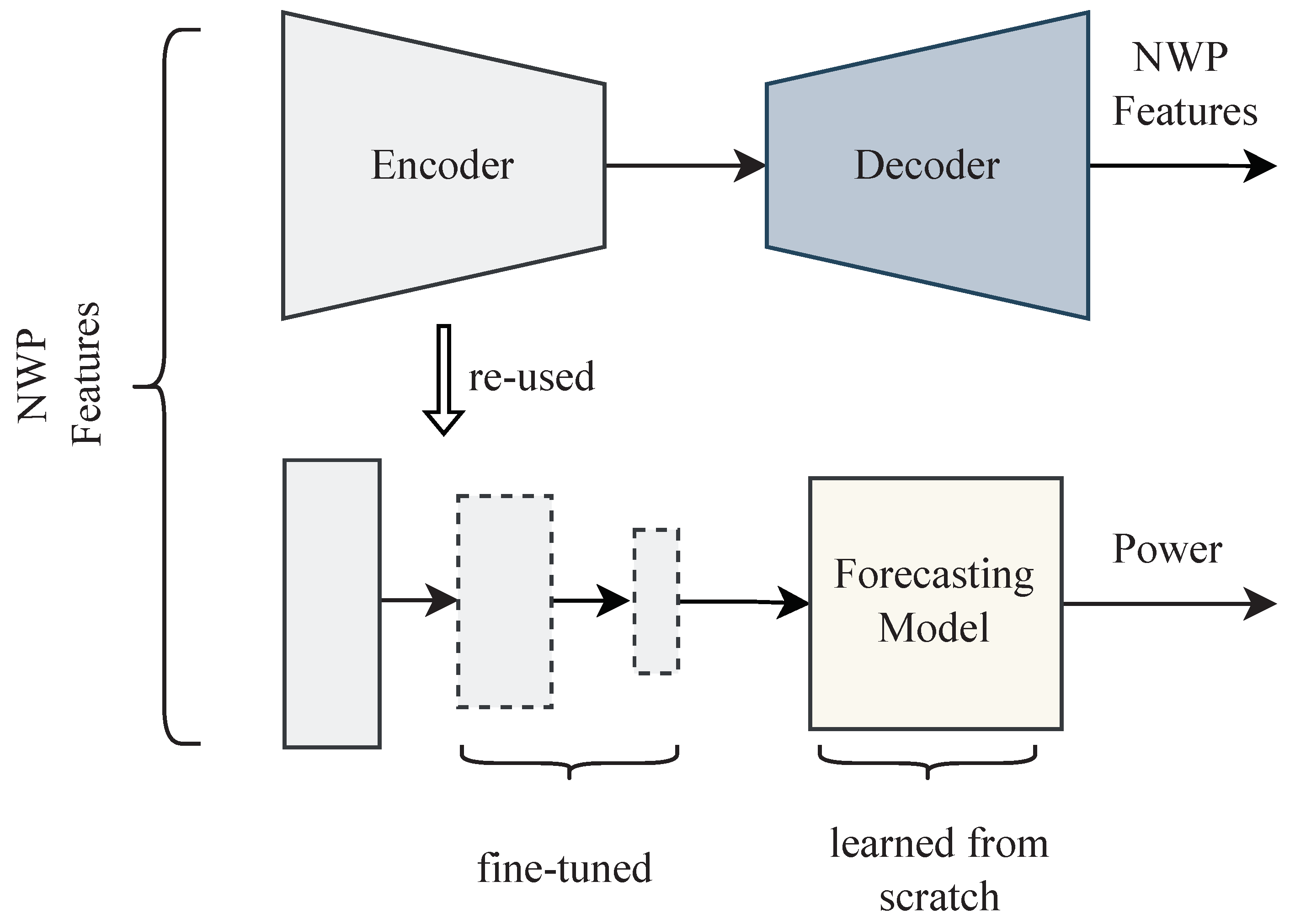
In our experiments, we initially trained an autoencoder to reconstruct the NWP features and learn the latent features of the weather. Afterward, the encoder was fine-tuned with a forecasting model to forecast the day-ahead power.
Figure 8.
In our experiments, we initially trained an autoencoder to reconstruct the NWP features and learn the latent features of the weather. Afterward, the encoder was fine-tuned with a forecasting model to forecast the day-ahead power.
Table 1.
Overview of the evaluated datasets. All datasets except PVREAL and WINDREAL are openly accessible.
Table 1.
Overview of the evaluated datasets. All datasets except PVREAL and WINDREAL are openly accessible.
| Dataset | #Parks | #Features | Mean Train
Samples | Mean Test
Samples | Resolution | NWP | Ref. |
|---|
| PVOPEN | 21 | 43 | 6336 | 8424 (57%) | hourly | ECMWF | [29] |
| PVSYN | 114 | 16 | 7596 | 3730 (32%) | hourly | ICON-EU | [30] |
| PVREAL | 38 | 25 | 14,513 | 4836 (25%) | hourly | ICON-EU | [31] |
| WINDOPEN | 45 | 9 | 6931 | 6659 (49%) | hourly | ECMWF | [29] |
| WINDSYN | 260 | 25 | 8428 | 4169 (33%) | hourly | ICON-EU | [30] |
| WINDREAL | 185 | 29 | 9032 | 3023 (25%) | hourly | ICON-EU | [31] |
Table 2.
Overview of autoencoder-based representation learning techniques. The model type is abbreviated as MLP for the multi-layer perceptron and TCN for temporal convolutional networks. MTL is an abbreviation for multi-task learning, where all parks of a datatype are trained in a unified autoencoder model. VAE is an abbreviation for a variational autoencoder as a generative approach for dimension reduction.
| Model Type | Architecture (STL or MTL) | Discriminative or Generative | Abbreviation |
|---|
| MLP/TCN | STL | Discriminative | AEMLP/AETCN |
| MLP/TCN | MTL | Discriminative | AEMLP-MTL/AETCN-MTL |
| MLP/TCN | STL | Generative | VAEMLP/VAETCN |
| MLP/TCN | MTL | Generative | VAEMLP-MTL/VAETCN-MTL |
Table 3.
The number of parameters for all autoencoder architectures for an example latent size of two. Other latent sizes solely differ slightly in the additional parameters required for the latent features. The number of parameters for the three wind and three PV datasets are summed for readability. The abbreviations here are the same as those in
Table 2.
Model Type
Data Type | AEMLP-MTL | AEMLP-MTL | AETCN | AETCN-MTL | VAE | VAE-MTL | VAETCN | VAETCN-MTL |
|---|
| PV | 118,707 | 3080 | 624,762 | 16,514 | 120,831 | 3116 | 629,718 | 16,598 |
| WIND | 421,870 | 2076 | 2,243,970 | 10,986 | 427,750 | 2112 | 2,257,690 | 11,070 |
Table 4.
Duration to train the different autoencoders in minutes. For the STL models, we trained with five parallel jobs. Each job utilized 20 CPUs and trained a single park. An MTL trained all parks simultaneously through a single job with 50 CPUs.
Table 4.
Duration to train the different autoencoders in minutes. For the STL models, we trained with five parallel jobs. Each job utilized 20 CPUs and trained a single park. An MTL trained all parks simultaneously through a single job with 50 CPUs.
| Model Type | Data Type | Duration |
|---|
| | | STL | MTL |
|---|
| AE | PV | 1473 | 1295 |
| | WIND | 5723 | 1126 |
| AETCN | PV | 5043 | 940 |
| | WIND | 13,174 | 1289 |
| VAE | PV | 1592 | 1309 |
| | WIND | 7456 | 1364 |
| VAETCN | PV | 5495 | 1009 |
| | WIND | 14,249 | 1342 |
Table 5.
Rank summary of the reconstruction error for all models and latent sizes for the autoencoder model (see
Table 2), and the PCA-based models. AEMLP is the baseline and all models were tested to determine whether the reconstruction error is significantly better (∨), worse (∧), or not significantly different (⋄) compared to the baseline. We test for a significant difference with the Wilcoxon test (
). The colors denote the respective rank. Blue indicates a smaller (better) rank and red a higher (worse) rank. The best latent size and data type model is highlighted in bold.
Data
Type | Latent
Size | Baseline | AEMLP-
MTL | AETCN | AETCN-
MTL | PCA | PCA-COSINE | VAE | VAEMLP-
MTL | VAETCN | VAETCN-
MTL |
|---|
| PV | 2 | 3.954 | 2.387∨ | 2.757∨ | 1.006∨ | 4.896∧ | 8.249∧ | 8.844∧ | 9.156∧ | 6.659∧ | 7.092∧ |
| PV | 4 | 3.682 | 2.971∨ | 2.410∨ | 1.087∨ | 4.850∧ | 6.173∧ | 9.069∧ | 9.474∧ | 7.451∧ | 7.832∧ |
| PV | 6 | 3.618 | 2.301∨ | 3.075∨ | 1.393∨ | 4.613∧ | 6.017∧ | 9.092∧ | 9.468∧ | 7.497∧ | 7.925∧ |
| PV | 8 | 3.254 | 1.983∨ | 3.983∧ | 1.260∨ | 4.520∧ | 6.006∧ | 9.017∧ | 9.538∧ | 7.486∧ | 7.954∧ |
| PV | 10 | 4.017 | 1.925∨ | 4.520∧ | 1.179∨ | 3.358∨ | 6.000∧ | 9.104∧ | 9.468∧ | 7.526∧ | 7.902∧ |
| WIND | 2 | 3.820 | 2.332∨ | 2.992∨ | 1.012∨ | 4.853∧ | 8.120∧ | 6.925∧ | 6.641∧ | 8.888∧ | 9.417∧ |
| WIND | 4 | 4.447 | 2.393∨ | 4.285∨ | 1.249∨ | 2.636∨ | 6.838∧ | 7.299∧ | 7.318∧ | 8.99∧ | 9.545∧ |
| WIND | 6 | 4.008 | 2.162∨ | 3.919⋄ | 1.110∨ | 3.813∨ | 6.401∧ | 7.376∧ | 7.553∧ | 9.081∧ | 9.576∧ |
| WIND | 8 | 4.080 | 2.037∨ | 4.439∧ | 1.000∨ | 3.458∨ | 6.165∧ | 7.256∧ | 7.570∧ | 9.222∧ | 9.773∧ |
| WIND | 10 | 4.014 | 2.199∨ | 4.828∧ | 1.002∨ | 2.970∨ | 6.103∧ | 7.387∧ | 7.501∧ | 9.231∧ | 9.764∧ |
Table 6.
Median nRMSE of the reconstruction error for all models and latent sizes for the autoencoder models (see
Table 2), and the PCA-based models. AEMLP is the baseline and all models were tested to determine whether the reconstruction error is significantly better (∨), worse (∧), or not significantly different (⋄) compared to the baseline. We test for a significant difference with Wilcoxon test (
). The colors denote the respective rank. Blue indicates a smaller (better) rank and red a higher (worse) rank. The best latent size and data type model is highlighted in bold.
Data
Type | Latent
Size | Baseline | AEMLP-
MTL | AETCN | AETCN-
MTL | PCA | PCA-COSINE | VAE | VAEMLP-
MTL | VAETCN | VAETCN-
MTL |
|---|
| PV | 2 | 0.126 | 0.108∨ | 0.112∨ | 0.075∨ | 0.141∧ | 0.201∧ | 0.227∧ | 0.227∧ | 0.190∧ | 0.191∧ |
| PV | 4 | 0.081 | 0.068∨ | 0.063∨ | 0.04∨ | 0.100∧ | 0.180∧ | 0.226∧ | 0.227∧ | 0.190∧ | 0.191∧ |
| PV | 6 | 0.058 | 0.046∨ | 0.052∨ | 0.028∨ | 0.072∧ | 0.153∧ | 0.227∧ | 0.227∧ | 0.189∧ | 0.191∧ |
| PV | 8 | 0.044 | 0.027∨ | 0.046∧ | 0.011∨ | 0.048∧ | 0.135∧ | 0.226∧ | 0.227∧ | 0.190∧ | 0.191∧ |
| PV | 10 | 0.042 | 0.015∨ | 0.044∧ | 0.014∨ | 0.024∨ | 0.124∧ | 0.227∧ | 0.227∧ | 0.189∧ | 0.191∧ |
| WIND | 2 | 0.119 | 0.109∨ | 0.110∨ | 0.081∨ | 0.135∧ | 0.255∧ | 0.217∧ | 0.214∧ | 0.276∧ | 0.278∧ |
| WIND | 4 | 0.103 | 0.080∨ | 0.097∨ | 0.062∨ | 0.088∨ | 0.209∧ | 0.213∧ | 0.214∧ | 0.276∧ | 0.278∧ |
| WIND | 6 | 0.068 | 0.054∨ | 0.067⋄ | 0.033∨ | 0.070∨ | 0.191∧ | 0.208∧ | 0.210∧ | 0.276∧ | 0.278∧ |
| WIND | 8 | 0.061 | 0.046∨ | 0.064∧ | 0.026∨ | 0.059∨ | 0.186∧ | 0.209∧ | 0.213∧ | 0.278∧ | 0.279∧ |
| WIND | 10 | 0.054 | 0.035∨ | 0.060∧ | 0.023∨ | 0.048∨ | 0.181∧ | 0.208∧ | 0.209∧ | 0.278∧ | 0.279∧ |
Table 7.
Rank summary of the forecast error for best models and latent sizes for the autoencoder models (see
Table 2), and the PCA-based models. AEMLP-MTL-MLP is the baseline and all models were tested to determine whether the mean performance rank was significantly better (∨), worse (∧), or not significantly different (⋄) compared to the baseline. We tested for a significant difference with the Wilcoxon test (
). The colors denote the respective rank. Blue indicates a smaller (better) rank and red a higher (worse) rank. The best model for a latent size and data type is highlighted in bold.
| Data Type | Latent
Size | Baseline | AEMLP-
MLP1 | AEMLP-
MTL-
MLP | AEMLP-
MTL-
MLP1 | AEMLP-
MTL-
MLP2 | AETCN-
MTL-
TCN1 | AETCN-
MTL-
TCN2 | AETCN-
TCN2 | PCA-
COSINE-
MLP | PCA-
MLP |
|---|
| PV | 2 | 6.821 | 6.682⋄ | 7.052⋄ | 5.665∨ | 5.780∨ | 2.503∨ | 2.480∨ | 4.671∨ | 6.775⋄ | 6.572⋄ |
| PV | 4 | 7.260 | 6.277∨ | 8.983∧ | 6.272∨ | 5.931∨ | 3.659∨ | 3.335∨ | 3.006∨ | 5.624∨ | 4.653∨ |
| PV | 6 | 5.514 | 5.445⋄ | 8.393∧ | 7.098∧ | 7.341∧ | 4.538∨ | 3.746∨ | 4.312∨ | 4.601∨ | 4.012∨ |
| PV | 8 | 6.936 | 5.746∨ | 8.220∧ | 6.110∨ | 6.491∨ | 4.965∨ | 4.046∨ | 5.121∨ | 4.035∨ | 3.329∨ |
| PV | 10 | 6.717 | 7.052⋄ | 6.023∨ | 6.422⋄ | 6.358⋄ | 5.225∨ | 4.133∨ | 5.017∨ | 3.838∨ | 4.214∨ |
| WIND | 2 | 4.707 | 4.440∨ | 6.606∧ | 3.778∨ | 3.830∨ | 5.349∧ | 4.641⋄ | 4.865⋄ | 9.683∧ | 7.102∧ |
| WIND | 4 | 6.312 | 6.341⋄ | 3.653∨ | 4.370∨ | 4.012∨ | 7.647∧ | 7.973∧ | 6.243⋄ | 4.366∨ | 4.083∨ |
| WIND | 6 | 5.212 | 3.992∨ | 7.574∧ | 5.805∧ | 4.954⋄ | 5.310⋄ | 4.239∨ | 4.031∨ | 7.160∧ | 6.723∧ |
| WIND | 8 | 4.879 | 4.989⋄ | 5.513∧ | 5.703∧ | 5.812∧ | 4.654⋄ | 4.071∨ | 4.627⋄ | 7.632∧ | 7.121∧ |
| WIND | 10 | 5.590 | 5.387⋄ | 6.130∧ | 4.346∨ | 4.039∨ | 5.007∨ | 4.121∨ | 4.320∨ | 8.018∧ | 8.041∧ |
Table 8.
Median nRMSE of the forecast error for best models and latent sizes for the autoencoder models (see
Table 2), and the PCA-based models. AEMLP-MTL-MLP is the baseline and all models were tested to determine whether the mean performance rank is significantly better (∨), worse (∧), or not significantly different (⋄) compared to the baseline. We tested for a significant difference with the Wilcoxon test (
). The colors denote the respective rank. Blue indicates a smaller (better) rank and red a higher (worse) rank. The best latent size and data type model is highlighted in bold.
| Data Type | Latent
Size | Baseline | AEMLP-
MLP1 | AEMLP-
MTL-
MLP | AEMLP-
MTL-
MLP1 | AEMLP-
MTL-
MLP2 | AETCN-
MTL-
TCN1 | AETCN-
MTL-
TCN2 | AETCN-
TCN2 | PCA-
COSINE-
MLP | PCA-
MLP |
|---|
| PV | 2 | 0.116 | 0.117⋄ | 0.116⋄ | 0.110∨ | 0.111∨ | 0.099∨ | 0.098∨ | 0.105∨ | 0.117⋄ | 0.116⋄ |
| PV | 4 | 0.099 | 0.095∨ | 0.106∧ | 0.092∨ | 0.093∨ | 0.087∨ | 0.087∨ | 0.087∨ | 0.093∨ | 0.092∨ |
| PV | 6 | 0.088 | 0.087⋄ | 0.094∧ | 0.090∧ | 0.09∧ | 0.086∨ | 0.084∨ | 0.085∨ | 0.087∨ | 0.085∨ |
| PV | 8 | 0.087 | 0.087∨ | 0.091∧ | 0.086∨ | 0.087∨ | 0.084∨ | 0.083∨ | 0.084∨ | 0.084∨ | 0.083∨ |
| PV | 10 | 0.087 | 0.087⋄ | 0.085∨ | 0.085⋄ | 0.087⋄ | 0.085∨ | 0.084∨ | 0.085∨ | 0.083∨ | 0.083∨ |
| WIND | 2 | 0.178 | 0.176∨ | 0.191∧ | 0.171∨ | 0.173∨ | 0.179∧ | 0.176⋄ | 0.178⋄ | 0.226∧ | 0.192∧ |
| WIND | 4 | 0.158 | 0.159⋄ | 0.143∨ | 0.146∨ | 0.145∨ | 0.174∧ | 0.175∧ | 0.163⋄ | 0.150∨ | 0.149∨ |
| WIND | 6 | 0.137 | 0.135∨ | 0.143∧ | 0.139∧ | 0.138⋄ | 0.136⋄ | 0.135∨ | 0.135∨ | 0.147∧ | 0.147∧ |
| WIND | 8 | 0.136 | 0.135⋄ | 0.135∧ | 0.135∧ | 0.135∧ | 0.134⋄ | 0.133∨ | 0.134⋄ | 0.145∧ | 0.146∧ |
| WIND | 10 | 0.135 | 0.135⋄ | 0.136∧ | 0.133∨ | 0.133∨ | 0.133∨ | 0.133∨ | 0.133∨ | 0.147∧ | 0.149∧ |
| Publisher’s Note: MDPI stays neutral with regard to jurisdictional claims in published maps and institutional affiliations. |
© 2022 by the authors. Licensee MDPI, Basel, Switzerland. This article is an open access article distributed under the terms and conditions of the Creative Commons Attribution (CC BY) license (https://creativecommons.org/licenses/by/4.0/).


