Abstract
In this article, a dual-stage proportional integral–proportional derivative with filter (PI–PDF) controller has been proposed for a hybrid two-area power system model having thermal-, hydro-, gas-, wind-, and solar-based power generating sources. Superconductor magnetic energy storage (SMES) units to cope with the transient power deviations have been incorporated in both areas. Governor dead-band (GDB) is considered in the governor model of thermal, and a generation rate constraint (GRC) is considered in the thermal and hydro turbine models to analyze the impact of system nonlinearity. The parameters of the proposed control strategy are optimally tuned by deploying a newly developed bull–lion optimization (BLO) to maintain optimal frequency and power response during system load deviations. Variations in wind speed and PV solar irradiance data have been included to examine the effectiveness of the BLO-based PI–PDF controller with system uncertainties and variability of renewable energy sources. The obtained results are validated by comparison with recently developed existing optimization techniques. The results revealed that the proposed control strategy is efficient for regulating the frequency and tie-line power of renewable integrated power systems. Further, the BLO-based PI–PDF control strategy improved the performance in terms of performance indices like settling time and peak overshoot/undershoot in wide scale.
1. Introduction
1.1. Motivation and Incitement
The capacity of electric utilities and the number of their connections are growing in the modern world, creating a complicated power system. These power systems are separated into several control areas, which are linked to one another by tie-lines. The areas of such rated power capacity are determined by the ratings of their synchronous generators [1,2]. The basic need of a complex power system is to design a controller that maintains the balance between the total power generation and the total energy consumption. Few variances among load demand and generation lead to deviation in frequency associated to its steady-state measure. A substantial reduction in frequency can cause instability. The swapping of power with the existing tie-lines operating at thermal limit shows low-frequency oscillation and thereafter, an unsystematic change in load and transients in renewable energy resources can cause large oscillation. The frequency oscillations can be abridged by applying the appropriate control for frequency regulation in the coupled power system and returning the area frequency and the power in the tie-line within the range of a desired limit [3]. The average time to regulate area control error should be kept to a minimum to quickly restrain the stable state and regulate the frequency profile with random load disturbances. Therefore, an improved LFC development is essential [4]. The main intention of LFC is to make sure that the frequency and inter-area tie-line power are within tolerable levels to control the disturbance and demand [5]. This assists in controlling the frequency and voltage of the system so that it is within the range of the preset limit as providing an acknowledged rate of power quality [1].
The frequency is maintained within the limit by the controllers in the network system and it also manages the power exchange. Both the reactive and active demands vary incessantly with the dynamic variation in load thereby generating oscillations. The oscillations can be promptly attuned to the normal level due to the presence of automatic generation control (AGC). The frequency involved in the power system oscillates due to the mismatch in load, generation, and losses in the system. This may lead to swinging power in the tie-line network among various regions. The system dynamics are required to be stable, which is attained through managing the tie-line power and also the generator’s output. This restrain is generally termed the area control error (ACE). Three key purposes of AGC are that the oscillations in the frequency, that tie-line power of the system must recline within an acceptable range, and that the working of the generation system is economical. In the paradigm of the multi-area power system (MAPS), various research analyses were known for LFC of the system working under different operating states [6].
1.2. Literature Review and Research Gaps
The performance of LFC can be improved, and until now, various restrain algorithms were used by a number of researchers. The performance of an artificial neural network [7], fuzzy logic controller [8], state feedback controller [9], sliding mode controller [10], and so on, are also analyzed for enhancing the performance of LFC. It is clear that from the review, a proportional–integral (PI) controller or its variants remain familiar due to various practical applications. The accomplishment of the appropriate maneuver of LFC is extremely dependent on choosing the parameters of the controller as an inappropriate selection may result in power system instability. In this framework, a number of evolutionary algorithms (EAs), such as differential search algorithm (DSA) [11], grey wolf optimization (GWO) [12], bat algorithm [13], and so on, have been employed for optimizing the gains of the controller to attain enhancement in the performance of the system. The efficiency of krill herd algorithm (KHA) for tuning the parameters of LFC was given in [14]. The comparative outcomes given in [15] show the effectiveness of KHA when compared to PSO and genetic algorithm (GA). In [16], an imperialist competitive algorithm (ICA) was utilized to balance the metrics involved in the PID controller for the LFC of the power system. However, the above stated strategies may have drawbacks such as a very slow rate of convergence, premature convergence, and input parameters dependence [17].
To increase the LFC performance, SMES and thyristor-controlled phase shifters (TCPS) are introduced into the control area. The operation of SMES–TCPS captures the initial drop in frequency and tie-line power deviance under abrupt load disturbance [18]. Further, a unified power flow control (UPFC) is employed in the tie-line, and SMES units are integrated in both areas. The frequency response of the proposed power system improves ominously with the projected UPFC and SMES units [19]. A SMES unit, which is capable of governing active and reactive powers instantaneously [20], is anticipated as one of the most effective tool for frequency oscillations. The feasibility of SMES for power system dynamic performance enhancement has been stated in [21].
Because electrical energy cannot be stored in excess, its generation and consumption must always be equal. This equation highlights the need for more controllers to take into consideration the integration of renewable energy sources into the conventional power system and is the key to effective management of any power system [22]. The LFC issues in realistic, two-area, single-source thermal units have been dealt with via a self-adaptive multi-population elitist (SAMPE) Jaya optimizer-based PID controller. The PID controller parameters has been perfectly tuned using SAMLE–Jaya optimization [23]. Further, a coyote optimization algorithm (COA)-based proportional–derivative with a filter cascaded-proportional–integral (PDn–PI) controller has been proposed for the PV and windfarm interconnected power systems. The control technique has been validated with some other existing techniques. The proposed technique provides a better dynamic performance in terms of frequency and tie-line power deviation [24]. The enhanced coyote optimization algorithm (ECOA)-tuned cascaded PDn–PI controller has been proposed for a solar–thermal-based two-area hybrid power system. The proposed strategy performs better than the other compared techniques [24]. A multi-area hybrid renewable NPS is proposed in [25] to examine the system nonlinearity, a GDB is instigated in the governor model, a GRC is considered with the turbine model, and a communication delay time (CDT) of phase determining tool is accomplished in the secondary LFC loop. A particular model is designed to take into consideration the outcome of cross-coupling between the LFC loop and excitation control system. Single- and multi-objective functions are executed to check the strength of the projected controllers. To obtain more practical results, actual wind speed, and sun irradiations data are taken in the wind model and photovoltaic model that were taken from a field study.
In a hybrid NPS with a deregulated environment, a grasshopper-optimization-based 3-degree-of-freedom (3DOF)–PID controller has been used to provide the best solution to the automatic generation control (AGC) problem. The control-of-power flow through PID and 3DOF–PID controllers has been investigated in order to adjust for load disturbances and control frequency oscillations. Then, a two-area AGC system is adopted, with a thermal hydro plant and a wind power plant in area-1 and a thermal hydro plant and a solar thermal power plant (STPP) in area-2. Additionally, the effectiveness of various FACTS devices, including UPFC and SMES, with the proposed controller AGC is compared to PID controller [26].
The primary aim of this research is to advance a strategy related to load frequency control automatically for a two-area NPS along with diverse sources. The proposed model consists of the various sources, such as gas turbine, hydro, and thermal power plants. Further, wind and solar are also incorporated. The significance of the research relies on the optimal tuning of the controller metrics and SMES parameters using the developed BLO algorithm that inherits the crossover and mutation characteristics of bull search agents [27] and the solitary and cooperative behavior of lion search agents [28]. The controller metrics are finetuned by minimizing the ITAE measure to make sure the power of the tie-line and the frequency of the multisource power system whereby in the bearable control. The results deliberate the effectuality of the proposed novel algorithm for the optimal modulation of the metrics of the proposed controller.
The discussions related to the regulation of frequency in the existing power system models are as follows: a hybrid optimization technique has been developed using the gravitational search algorithm, the firefly algorithm, and particle swarm optimization. It was observed that the proposed technique outperformed the other three well-known techniques, which were PSO, FA, and GSA [6]. The parameter of the PID controller has been optimized and convincing results have been obtained, but the proposed optimization provides slow convergence and variation in the frequency and tie-line power is also high. In [29], the jump system theory was introduced that efficiently enhances the performance of control dynamics over error in power and random delay in communication, while assuring the stability of networked LFC closed-loop. However, the rate of PMU data sent within a restricted time period is controlled by transmission. The marine predators algorithm is used in [30], which illustrates an excellent performance in handling the penetration of energy storage and RES, whereas the achieved results are oscillating in between the tolerable boundary with respect to the regulations of the European grid. However, the controller employed in the analysis is considered as a basic PID controller with filer, comprising of four gain coefficients. Proportional gain Kp is the first, which minimizes the steady-state error and rise time but increases in Kp affects the stability of the system. In [31], a quasi-oppositional dragonfly algorithm is developed. The strategy used is quite efficient to evaluate the optimal gains of PID in the performance of LFC. However, it may produce results with poor accuracy, result in convergence to local optimal values, and presents difficulty in finding the global optimal solution.
1.3. Contributions and Paper Organization
- LFC of a two-area diverse sources realistic power system that consists of a thermal, hydro, and gas power plant in each area considering system nonlinearities, i.e., GRCs, GDB, and CDT are investigated. A HVDC link has also been included in the model for improving the dynamic response. Further, the RESs, i.e., WTG and PV solar, are integrated in the present system and the model is investigated with a different scenario.
- A novel control scheme PI–PDF controller with coordination of SMES–SMES has been proposed to investigate the dynamic response of the stated system.
- A developed BLO technique for optimizing the proposed controllers and the SMES parameters to ensure the frequency regulation of stated power system.
- To assert the efficacy and robust performance of the proposed control strategy, step load perturbation (SLP), and random load probation (RLP) are checked with RESs on the power system model.
- The random wind and solar data have been considered to check the efficacy of the proposed control strategy for the stated power system.
The manuscript is structured as follows. Section 1 provides a short introduction and explains the related work regarding the paper. Section 2 presents the proposed power system. Section 3 explains the proposed method of controlling the load frequency in the power system. Section 4 covers the selection of the optimization techniques. In Section 5, the result analysis is deliberated. Finally, in Section 6, the conclusion of the presented paper is given.
2. Proposed Power System
Having almost all the power systems generally coupled to their adjacent areas, where the issue of regulating frequency based on the load, is a major task. The considered power system, as presented in Figure 1, is a two-area interconnected hybrid power system that contains a reheat turbine thermal power plant (RTPP), hydropower plant (HPP), and a gas power plant (GPP) in each control area, as shown in Figure 1. The power rating of each area is 2000 MW and nominal loading is 1740 MW, RTPP provide 1000 MW, GPP contribution 240 MW, and HPP delivering 500 MW. Further, the specification of the presented system and its parameters are stated in Appendix A [32]. Further, the physical constraints such as GRC and GDB of the power system for non-linearity and a more realistic study are considered of the thermal units, where GRC rate is taken (0.003 pu/s and 0.0017 pu/s). In addition, the GRC of the HPP is (0.045 pu/s) and (0.06 p.u.) for increasing and decreasing rates, respectively. The GDB non-linearity equations can be linearized in terms of rate of change and speed of change [33]. The transfer function that is considered for GDB with 0.5% backlash is achieved by Fourier series is given below in Equation (1):
where, , are the Fourier coefficients. The value of Tsg is mentioned in Appendix A. Communication delay time (CDT) is considered as 0.03 sec in each area. Each source has major components, such as generator and governor turbine. These components are derived in proceeding section.
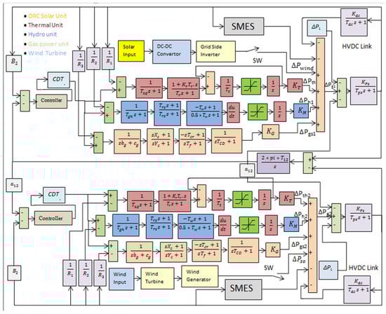
Figure 1.
Power system model.
2.1. Modeling of Generator
The generator converts the mechanical power generated by the turbine into electrical power. Relation among the electrical and the mechanical power is formulated by the swing equation related to the synchronous machine to small uncertainty, and is given as:
where, represents the deviation in rotor speed, indicates the constant inertia, is the variation in mechanical power, and is the deviation in electrical power. Different types of electrical components constitute the load in a power system, which may either depend on the deviation in frequency or not. The relation of electric power based on the change in frequency is formulated as:
where, represents the load change independent of frequency, and denotes the sensitive load change with frequency. In a multimachine system, with the presence of three generating power units, such as a hydropower system, gas-turbine, and thermal power system, working in parallel condition in the same area, and all the generators are assigned with the equal speed of synchronism. The equivalent load-damping constant and the equivalent generator inertia constant is formulated as:
The expression for equivalent generator is expressed as:
where, D is the damping constant, M is inertia of generator, ∆F is change in frequency, and represents the power generating units, such as the hydropower system, thermal power system, and gas-turbine power system.
2.2. Modeling of Governor-Turbine
The governors indicate a valve that manages the rate of steam or fuel that is passing into the system. On the other hand, the turbine is a mechanical device to convert the thermal power from the governor into mechanical power. In order to regulate the frequency into a nominal value, it is needed to maintain constant rotor speed; the turbine valve is adjusted by each generator with the governor. The mathematical expressions for this model are given as:
where is governor output power change and is the turbine time constant change in mechanical output.
2.3. Modeling of Tie-Line
Generally, in multi-area power systems with interconnections, the number of areas is connected with one another through the tie-lines; thus, the flow of power among these areas is performed by the connected tie-lines.
Considering the power flow of the tie-line from area i to j, the variation from the nominal flow is formulated as:
where and are the change in rotor speed of area-1 and 2.
2.4. Modeling of Load Frequency Control
The prime target of the LFC loop is to regulate the reference working point of the governor units in the location of control and set their outputs. The actual frequency and total exchange of power flow are evaluated for the estimation of the requirement of area with the use of independent system operator. Expression for the area control error is formulated as:
where, denotes the response of frequency characteristics for the area i. The equivalent frequency bias factor in the multi-generator system cases is expressed as:
The control-of-power flow in tie-line power and frequency are important to sustain the power system stability. The variations of tie-line power and frequency of power sources, such as gas-turbine, thermal, and hydro power plants, are needed to be minimized in order to balance the power and frequency of the system at the scheduled values.
2.5. SMES Unit
Figure 2 shows the fundamental configuration of the SMES unit taken into account for the suggested system. During the utility grid’s routine operation, the superconducting coil can be charged from the grid to a predetermined value (i.e., less than the full charge). A power converter (PC), which consists of an inverter/rectifier, connects the magnetic coil to the main grid. When a superconducting coil is charged, it conducts current nearly damage free, supporting the electromagnetic field. By dipping the coil in liquid helium, the coil is kept at a very low temperature (less than the critical temperature). The stored energy is immediately released to the grid through the PC in the form of high-quality AC power when there is a rapid spike in load demand. The coil charges back up to its original value as the governor and other controller functions begin to bring the power system into equilibrium. A similar behavior was reproduced during a sudden load reduction. As the system returns to its steady state, the absorbed excess energy is released, and the coil current returns to its normal value. The coil instantaneously charges towards its absolute value, capturing part of the system’s excess energy [19,34]. The SMES model as a frequency regulator is designed as a second-order lead-lag compensator and presented in Figure 3. SMES is coupled at the opposite load as shown in the proposed power system model. For SMES–SMES coordination, each area has six parameters such as regulation gain, K_SMES and time constants T_SMES, K1, K2, K3, and K4 to be tuned for the optimal design of a coordinate frequency regulator.
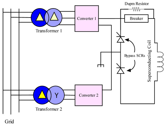
Figure 2.
Structure of SMES unit.
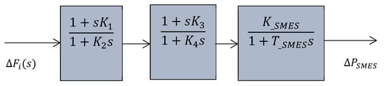
Figure 3.
Modelling of SMES as a frequency controller.
2.6. DC Link
The DC link system helps in decreasing the tie-line power and frequency deviation by regulating the corresponding DC power flow. The DC link increases the dynamic response of the system [35]. The DC link is fitted parallel to the AC line in each of the control areas and represented in the Equation (11).
where, GDC is the overall gain of DC Link, Kdc, Tdc are gain constant and time constant of DC link.
2.7. PV System
In this study, PV modules are mathematically described using a single-diode PV model. This is as a result of its precision and clarity. The PV module’s nonlinear I–V characteristic is expressed as follows [36,37]:
where Rs and Rp are the series and parallel resistances, IPV is the photovoltaic current, Io, and a are the diode’s reverse bias current and ideality factor, respectively, and Vt is the thermal voltage.
In this work, a large-scale 50 MW PV system is created using the series–parallel connection approach. To interface the PV module with the stated power system, power electronic circuits, i.e., a grid-side inverter and DC–DC converter, are considered. Transfer functions with a unity gain and a 10 ms time constant are used to simulate these interfaced circuits.
2.8. Wind Turbine Energy System
The captured energy of blowing wind changes mechanical energy over to electrical energy with the help of a wind turbine. As the unstable nature of wind is not predictable, so too does the extractable power of a wind turbine generation depend on the speed of the wind. It normally incorporates a gearbox, and some wind turbines use edge pitch system controllers to control the aggregate sum of the changed force. The electrical generator changes mechanical energy into electrical energy [25]. The power captured from wind Pm can be mathematically expressed in as follows:
where is air density, r is radius of blade, Vm is wind speed, λ tip is speed ratio, β is pitch angle of blade, and the power coefficient Cp can be derived as [38]:
where, is blade speed.
A wind farm of rated capacity of 85 MW, which is integrated with the system, is presented in Figure 1. The inputs on the wind are considered as constant and random data. The wind induction generator is statistically demonstrated by a transfer function of a unity gain and 0.3 s time constant. The pitch control is utilized for tracking the maximum power.
3. Proposed Control Strategy
Due to the continuously changing operating point of the power system, a fixed controller is not appropriate in all the operating states [26]. Hence, it is necessary to develop a controller that operated in all the operating states with enhanced efficiency. The controller in the power system regulates the frequency deviation from the scheduled value. Hence, the researchers are focused on searching for a suitable control method to stabilize the frequency deviation. In this work, the performance of the system is examined with two different types of controllers, i.e., PIDF, and PI–PDF. Further, the dual-stage control strategy can handle multiple disturbances more efficiently that improve the performance of the system.
3.1. PI–PDF Controller
The controller is utilized to identify an appropriate set of controls that can make the system reach the expected state smoothly and with reduced deviations. Generally, the equations of control systems are complex, and hence the controller must be capable of incorporating the modeled effects and nonlinear properties into its design. One of the most common industrial controllers is the PID controller, which possesses enhanced properties and established design strategies.
The PI–PDF controller is dual-stage control strategy that can handle multiple disturbances more efficiently which improve the performance of the system. In such a dual-stage control strategy, a combination of the two controllers is presented in Figure 4, in which the first stage has a PI controller and the second a PD controller with the filter coefficient Nff. The PI is connected in the first stage and its output will act as a set point input for the second stage PDF controller. The transfer function of the PI–PDF controller is presented in Equation (15) U= for load disturbances where disturbance is defined as [39].
here, KP; KI; KPP; KDD, and NFF are the parameters that are to be tuned by various optimization techniques.
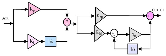
Figure 4.
Configuration of proposed controller.
The controller’s gains have been optimized subjected to minimizing the cost function defined in Equation (18) by deploying BLO optimization.
3.2. Automatic Generation Control
For improving the operation involved in the power system under different working states, the tuning of the PI–PDF controller metrics in an optimal way is necessary. The uncertainty and the dynamic variations of the model are expected to be handled by optimally tuning the PI–PDF controller parameters. The power system must be very sensitive to the changes in perturbation of the loads and track the expected point for all the variables. Over the number of performance indices that evaluate the effectiveness of the power system, ITAE is found to be the one that provides satisfactory results for the parametric optimization based on the settling time and overshoot. Hence, in the proposed work, ITAE is considered as the target function to be minimized, and the expression of ITAE in relation to a two-area power system is expressed as:
where, denotes the variation of power in tie-line, ∆F1 indicates the changes occurring in frequency corresponding to area-1, and ∆F2 represents the variation in frequency corresponding to area-2. The objective function ITAE is minimized by the proposed BLO algorithm for analyzing the PID controller parameters. The constraints to be followed are, , , , , and . In addition, the time domain representation of proposed controller becomes:
where, Y1 and Y2 are the controller output of both areas and area control error represented as below in Equations (1) and (2):
From Equations (21) and (22), it is clear that ACE depends on the deviation in frequency and the power in tie-line for the proposed model. The parameters of the PI–PDF controller are tuned optimally using the proposed BLO algorithm in such a way as to control the variation in frequency and the power in tie-line, with ACE being the input to PI–PDF controller. The Simulink implementation of the developed two-area power system is presented in Figure 1.
3.3. Artificial Intelligent Technique for Controller Design
A power system’s controller is an essential component whose performance has a direct impact on the results. The controller design is also founded on complicated, mix-integrated equations. Therefore, for better results, it demands suitable and optimal parameters. AI-based optimization strategies are well defined to handle such engineering challenges, according to the well-known literature [4,25,40]. It should be emphasized that according to [41] no optimization technique can be used to solve all problems; therefore, a specific optimization technique may work better for one type of solution but not for another. This implies that a search for a suitable optimization approach for a specific type of optimization problem is needed.
3.4. Proposed BLO Algorithm
A hybrid metaheuristics technique called the BLO algorithm has been proposed using the combined properties of various search agents, such as bull search agents [17,25], and lion search agents [18] based on the optimal tuning of the PID and proposed PI–PDF controller parameters. The majority of common optimization algorithms are created based on the hunting characteristics of search agents that help the search agents find their target. Similar to this, the suggested hybrid BLO algorithm demonstrates the cooperative and crossover characteristics of the lion search agents as well as the characteristics of the bull search agents when they are hunting prey. The unique lifestyle of the lion search agents results in improvements to the suggested algorithm. The suggested BLO algorithm can be widely applied to obtain the global optimal measure at a low computation cost and high level of accuracy. The proposed hybrid BLO algorithm increases the likelihood of finding the solution to the optimization problem. As a result, the suggested algorithm is better able than single optimization techniques to arrive at the global optimal solution with a faster rate of convergence.
- (a)
- Inspiration for the development of proposed BLO algorithm
In general, most of the engineering-based optimization problems are quite complicated to resolve, and the applications have to handle complex problems. In these problems, the space of search increases exponentially with the size of the problem. Hence, the conventional optimization strategies do not offer an appropriate solution for such problems. Thus, in the former times, the number of metaheuristic algorithms have been developed to solve similar problems. Lion search agents are the most communally biased of all species of wild cats that show a high range of opposition and cooperation. Lion search agents are of more concern due to their tough sexual dimorphism in both social appearance and performance. The lion is an undomesticated creature with two kinds of social organization, such as nomads and residents. Residents survive in factions, called a pride, where a pride of lion search agents characteristically comprise one or more adult lion search agents, five females, and their cubs.
Young search agents are eliminated from their birth pride when they grow sexually adult. On the other hand, the nomads move infrequently, either as singular or as a pair. Pairs are seen more between related males who have been removed from their maternal pride. It must be noticed that a lion search agent may change its lifestyle from resident to nomadic and from nomadic to resident. Similarly, the bull search agents possess the selection property that enhances the velocity of the lion search agents in the hunting of prey when incorporated with the characteristics of the lion search agents. The steps followed by the BLO algorithm are explained as:
- Step 1:
- Objective function: The proposed BLO objective is to minimize the measure of ITAE. The tuning of the PID metrics is achieved by reducing the main intention function. The objective of the developed optimization problem is represented as Min (ITAE).
- Step 2:
- Parameters initialization: As the first step, the numbers of male lion search agents , female lion or lioness search agents , and the nomad lion search agents are initialized. In addition, initialize with maximal computation of iterations. Individual lion searching agent possesses the position vector indicating the current position as:where, indicates the population of the male lion search agents in the search space.
- Step 3:
- Fitness evaluation: The ITAE generated by each lion search agent is considered as the fitness of each solution and is evaluated for all the lion search agents. All the lion search agents are sorted based on their fitness measure in such a way to evaluate the best lion search agent. The fitness value of each lion search agent is stored as:The corresponding fitness measure of each lion search agent is stored in the form of the above equation that determines the survival of the fittest.
- Step 4:
- Generation of pride: The nomadic lion search agent is not a member of the pride, and the representation of the male lion search agent is the solution vector representation. The vector elements of , and , that is and , are the arbitrary integers within the maximum limit and the minimum limit for the search with real encoding with . The length of the lion search agent can be evaluated as:where, and are the deciding integers that decides the lion length. The algorithm searches with the binary encoded lion search agents for the condition when , and hence the element of the vector is produced either as 0 or 1, with the constraints as given below:where, the Equations (26) and (27) indicate that the produced binary lion search agent lies within the search space. According to Equation (28), the number of binary bits after and before the decimal points is equal. With the assumption that there are two nomadic lion search agents to invade the territory, the fills one of the two positions of the nomadic lion search agents. The remaining one is called only during defense for territory, and the position becomes null, which is represented as .
- Step 5:
- Evaluation of fertility: In the sequential process, the male lion search agents and the female lion search agents begin to age or become infertile. Thus, the lion search agent become slacker and may get defeated at a terrestrial takeover by the nomad lion search agents. At this point, the lion search agents become saturated with the achievement of either the local optimal or the global optimal and may be unable to provide any other enhanced solutions. When the reference fitness is less that the fitness of the fitness of the male lion search agent, then is found to be a slacker, and the slacking rate is increased by 1. With the value of slacking rate exceeding its maximum limit, , then the territorial defense takes place. On the other hand, the fertility of the female lion search agent is assured by the sterility rate , which is incremented by one after crossover. When the value of exceeds its maximum limit , then the female lion search agent is updated as:where, and are the and vector elements of , respectively, is a random integer generated between the 1 and , is an update function of female lion search agent, and are the random integers that varies from 0 and 1. When there is any improvement in the female lion search agent, then the mating process takes place. Similarly, if there is no female lion search agent to replace the existing one, is assumed to be fertile enough. On the contrary, when the updated female lion search agent is considered as the female lion search agent, mating takes place with the updated female lion search agent.
- Step 6:
- Hunting for survival: The female lion search agents always look for prey to feed the members of the pride. During the hunting process, the female lion search agents adjusts their position based on their own location or the location of the members in the pride. The position of the prey is expressed as:where, is the position of the hunter or the female lion search agent at iteration, is the position of the prey, is the random number ranging between 0 and 1, and is the percentage of enhancement in the fitness of prey. The position of the female lion search agent is formulated as:where, is the velocity of hunting process that can be boosted with the integration of the selection property of the bull search agent, and in such a way as to enhance the hunting process of the female lion search agent.Thus, the position of the prey is formulated as:where, is the inertia constant, , and are the randomized numbers which range from 0 to 1, is the personal or local best solution of female lion search agent, is the worst solution, is the best directional leading position so far, and is the global best solution.
- Step 7:
- Mating process: The mating process involves crossover and mutation as the initial step, followed by which the gender grouping takes place as the final step. A maximum of four cubs is assumed to be the given birth by the female lion search agent at a single time, where the four cubs again undergo mutation and crossover operations to form four more cubs. Hence, the cubs obtained through crossover are represented as and the cubs obtained through mutation are represented as . The total of 8 cubs are then made to gender clustering to separate them as male cubs and female cubs .
- Step 8:
- Operators of lion search agents: The territorial defense assists the algorithm not to fall in local optimal solutions. The nomad lion search agent is selected when its fitness is less than the male lion search agent, male cub, and female cub. When the male lion search agent gets defeated, the pride is updated, and when the nomad lion search agent gets defeated, the nomad coalition is updated.
- Step 9:
- Termination: The algorithm is terminated once when completing the maximal countable iteraftions, at which the globally suitable solution is obtained. The pseudocode of the developed BLO algorithm is presented in Algorithm 1.
| Algorithm 1: Pseudocode of proposed BLO algorithm | |
| S. No. | Pseudocode of proposed BLO algorithm |
| 1 | Input: |
| 2 | Output: |
| 3 | Initialize the population of lion search agents |
| 4 | Initialize maximum iteration |
| 5 | T = 0 |
| 6 | While T < maximum iteration |
| 7 | Evaluate fitness for all lion search agents; |
| 8 | For all lion search agents |
| 9 | Generate pride |
| 10 | Evaluate fertility |
| 11 | Hunting for survival |
| 12 | Evaluate position of female lion search agents based on velocity of bull search agents |
| 13 | Update the position of prey using Equation (35) |
| 14 | Perform mating process |
| 15 | Obtain cubs |
| 16 | Perform gender clustering for cubs |
| 17 | Perform cub growth function |
| 18 | Perform territorial defense |
| 19 | Update the male and female lion search agents |
| 20 | End For |
| 22 | Set |
| 23 | End while |
| 24 | Return |
4. Selection of Optimization Technique
To manifest the efficacy and potential of the developed BLO to solve the problem of controller design for a power system, a simple problem of frequency controller for the power system is considered with a single objective of minimization of the error function. The problem is solved by deploying six optimization techniques for a better analysis. Considering the randomness associated with these metaheuristic AI techniques, a 20-run independent trial is performed with 100 iterations and 30 populations and is provided in Table 1. The table summarized the elementary value of worst, mean, and best obtain fitness along with the standard deviation (SD). This can be studied from the state table that BLO has presented impressive results compared to other well-known optimization techniques for the PID controller. The promising results are highlighted. Further, for more analysis, the convergence characteristics of all compared techniques are obtained and presented in Figure 5a and Figure 6a for the same controller and similar objective. This can be the analysis from the figure that compared techniques which are trapped in the local optimal whereas the BLO has effectively obtained the global optimal for the stated problem. It can be analyzed from this figure that BLO has an evenly distributed elementary solution with a lower median value as compared to other techniques. Considering the obtained results, the authors endorse BLO for solving the problem of frequency deviation in proposed the power system. The comparative optimization techniques are discussed in [5,8,27].

Table 1.
Statistical analysis for comparison of optimization techniques.
5. Simulation Results and Discussions
The results attained using the developed bull–lion dependent PI–PDF controller and the comparative evaluation for proving the superiority of the proposed strategy for regulating the power in tie-line and frequency in a two-area power system is discussed in this section.
An Intel i7 laptop with 16 GB of RAM was used to run the simulation study using the MATLAB/Simulink platform. Following the initial design of the PI–PDF controller using the BLO algorithm (see Appendix B) along with the SMES unit and HVDC link, the performance of the developed controller has been validated for operating the system under various scenarios that frequently occurs in real-time.
The following operational scenarios are considered for the system under study:
- Scenario-I
- In this section, the performance of proposed control strategy is studied with two-area, realistic no-reheat thermal, hydro, and gas power system considering nonlinearities like GRC, GDB, and CDT as mentioned above with a rated capacity of 2000 MW and 50% loading that has a 1% (0.01 puMW) load perturbation in area-1 is considered. Additionally, a SMES unit and HVDC link are integrated in each area for reliable operation of stated power system.
- Scenario-II
- In this section, the following power system is considered in scenario-I, and the system’s performance was further examined by integrating the RES units, i.e., wind turbine generation (85 MW) and PV solar (50 MW) with a fixed-step input (wind generation = 0.045 pu, and Solar generation = 0.025 pu).
- Scenario-III
- An RESs-integrated sated two-area power system is studied with the random load in area-1 and step load in area-2 along with random wind speed and solar irradiance.
- Scenario-IV
- A robustness analysis of a RESs-integrated power system for proposed control strategy is studied under consideration of change in system parameter.
5.1. Scenario-I
The investigation is expanded to a multi-source, two-area, thermal, hydro, and gas power system, presented Figure 1. Initially, a two-area, realistic, no-reheat thermal, hydro, and gas power system, considering nonlinearities like GRC for TPP (0.003 pu/s and 0.0017 pu/s), GDB, and CDT (0.03 s), with a rated capacity of 2000 MW and 50% loading, has a 1% (0.01 puMW) load perturbation in area-1, which has been taken into account. Additionally, SMES unit and HVDC link are integrated in each area for the reliable operation of the stated power system. The optimal parameters of the controllers and SMES unit obtained from the various algorithms are presented in Table 2. The obtained results are presented in Table 3. The settling time (F1_Ts, F2_Ts), undershoot (F1_Us, F2_Us), and overshoot (F1_Os, F2_Os) of the frequency response for area-1 and area-2 can be seen from the table, respectively. Moreover, Ptie_Ts, Ptie_Us, and Ptie_Os are settling time, undershoot, and overshoot for tie-line power deviation, respectively. It can be further seen from the table that the obtained values for these performance indicators are the best for the BLO base PI–PDF controller.
Table 2.
Optimized parameters of controller for scenario-I.
Table 3.
Time domain analysis for scenario-I.
Figure 5a presents the performance comparison of various controllers in the convergence characteristics. Figure 5a shows that the proposed controller performed best compared to the other compared techniques. Figure 5b–d present the frequency deviation of area-1, area-2, and tie-line power deviation, respectively. It can be analyzed from Figure 5b,c that the BLO: PI–PDF controller has performed best for the frequency deviation response for area-1 and area-2, as compared to other compared controllers. Further, Figure 5d presents the comparison of the dynamic response of tie-line power deviation. It can be observed from this figure that the BLO PI–PDF controller has generated impressive results, as compared to other mentioned controllers.


Figure 5.
Dynamic response of power system for scenario-I: (a) Convergence characteristics, (b) Frequency response of area-1, (c) Frequency response of area-2, and (d) Tie-line power response.
Figure 5.
Dynamic response of power system for scenario-I: (a) Convergence characteristics, (b) Frequency response of area-1, (c) Frequency response of area-2, and (d) Tie-line power response.


5.2. Scenario-II
Furthermore, to reflect a more practical approach in this scenario, renewable energy sources are integrated in both the area of power stated in scenario-I. The RESs are considered constant power sources [39] and step input is applied at time t = 0. This has been performed to test the framed controller for ideal conditions. A figure of 1% SLP has been considered in area-1. The optimal parameter for this scenario is presented in Table 4. The obtained results are presented in Table 5. It can be analyzed from the aforementioned table that, for this scenario too, the proposed controller minimizes the errors as compared to other controllers. The results are marked bold for clarity. Table 5 demonstrates the settling time (F1_Ts, F2_Ts), undershoot (F1_ Us, F2_Us), and overshoot (F1_Os, F2_Os) of frequency response for area-1 and area-2, respectively. Moreover, Ptie_Ts, Ptie_Us, and Ptie_Os are settling time, undershoot, and overshoot for tie-line power deviation, respectively. It can be further understood from this table that the obtained values for these performance indicators are best for the BLO-based PI–PDF controller. For further verification, the result obtained from the proposed controller is analyzed and presented below. Figure 6a presents the convergence characteristics for this scenario. The convergence characteristics reveal that the proposed controller achieves the best fitness for the proposed model. Figure 6b,c demonstrate the comparative dynamic response of frequency deviation in area-1 and area-2, respectively; whereas, Figure 6d denotes the comparative dynamic response of tie-line power deviation. It can be analyzed from Figure 5 that, for this scenario, the proposed BLO: PI–PDF controller has performed best for the frequency deviation response for area-1 and area-2, as compared to other compared controllers. Further, Figure 7a,b present the recorded power response of the sources for area-1 and area-2, respectively. Pth is the power generated by thermal unit and Phy is the power generated by the hydro unit, Pgas is the power generated by the gas unit, whereas Pso and Pwind are the power generated in solar and wind power generating units, respectively, and Psmes is the power flow in SMES unit. It is clear from Figure 7a that the sum of power generated (Pg) from the various sources is equal to the disturbance applied 1% (0.01 puMW) on area-1, whereas no disturbance has been applied on the area-2; therefore, in Figure 7b, the sum of all sources power (Pg) is zero. Hence, the proposed control strategy is working perfectly.
Table 4.
Optimal value of the parameters for scenario-II.
Table 5.
Time domain analysis of power system for scenario-II.
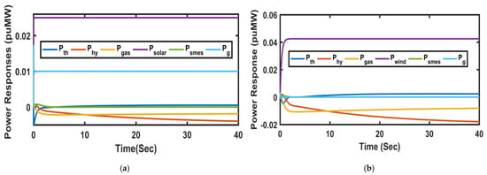
Figure 7.
Power responses of various sources of (a) area-1 and (b) area-2.

Figure 6.
Dynamic response of power system for scenario-II: (a) Convergence characteristics, (b) Frequency response of area-1, (c) Frequency response of area-2, and (d) Tie-line power response.
Figure 6.
Dynamic response of power system for scenario-II: (a) Convergence characteristics, (b) Frequency response of area-1, (c) Frequency response of area-2, and (d) Tie-line power response.

5.3. Scenario-III
In this section, a random load pattern is generated for area-1 and is presented in Figure 8a. Further, to reflect a more practical approach in this scenario, both renewable energy sources are taken as variable power generating sources and verified under solar and wind data, as presented in Figure 8 [42]. For further verification, the result obtained from the proposed controller is analyzed and presented below. Figure 8a,b demonstrate the solar irradiance and wind speed. Figure 8c,d demonstrate the comparative dynamic response of frequency deviation in area-1 and area-2, respectively; whereas, Figure 8e denotes the comparative dynamic response of tie-line power deviation. It can be clearly analyzed from Figure 8, for this scenario too, that the proposed controller minimizes the errors as compared to other controllers and demonstrates the settling time, undershoot, and overshoot of the frequency response for area-1 and area-2, and that the tie-line power deviation is much less compared to another compared controller. It can be further seen from Figure 8 that the obtained results for these performance indicators are best from the BLO-based PI–PDF controller. Hence, the proposed control strategies perform best and suppress the frequency oscillation more rapidly with much less overshoot and undershoots.
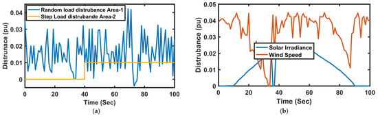
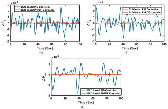
Figure 8.
(a) Disturbance applied on area-1 and area-2, (b) Solar irradiance and wind speed, (c) Frequency response of area-1, (d) Frequency response of area-2, and (e) Tie-Line power response.
5.4. Scenario–IV
In this section, to check the robustness and sensitivity of the proposed controller, the parameters of the study system have been varied within the range of ±25% without a change in the optimal values of the controller gain. These variations include the governor, turbine, reheater, droops, and frequency biases’ time constant values (area-1 and area-2). The power system’s operating load conditions and the synchronization coefficient are also varied. The recorded dynamic responses in Figure 9 make it clear to the reader that the BLO-based PI–PDF controller was effective even when system parametric changes were present. It can be claimed that the analysis presented above demonstrates the suggested controller of LFC’s viability for a wide range of system parameter and operational load situations. Figure 9a,b present the system comparison for step load changing area-1 at nominal and varied conditions and Figure 9c is the power deviation response. It can be easily seen from Figure 9 that the settling time and peak overshoot values vary within acceptable limits and are comparable to the respective values obtained with nominal system parameters. It can, therefore, be concluded that the proposed controller approach has impressively provided a robust and stable operation.
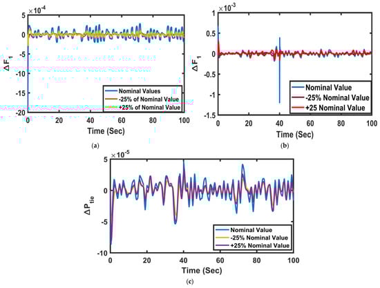
Figure 9.
Dynamic Response of a system for scenario-IV: (a) Frequency response of area-1, (b) Frequency response of area-2, and (c) Tie-line power response.
6. Conclusions
In this study, for the suggested two-area power systems, the proposed BLO-based dual-stage PI–PDF controller is perfect for achieving load frequency control and minimizing the tie-line power variation. The established BLO approach, which inherits the bull search agent’s selection property and the lion search agents’ cooperation behavior, is important because it enables the best controller metric tuning. When taken into consideration, the metrics to determine if the suggested BLO-based PID controller approach is effective are the fluctuation of frequency in area-1 and area-2 as well as the tie-line power. Initial testing of this controller’s capabilities is performed on a recognized two-area thermal, hydro, and gas PS with the effects of GDB and GRC nonlinearity, and then on considering SMES a HVDC link. Several findings are provided to support the effectiveness and benefits of the suggested control technique. Comparing the controller’s responses with those found in the literature also prefigures its superiority. The same PS models subjected to SLP of the same setting and magnitude are taken into account while conducting assessments in fair conditions. Further, the proposed controller has been studied for the stated PS integrated with the RESs. The system performance with the BLO: PI–PDF controller is superior to that obtained by traditional PID controllers, according to the simulation findings. The suggested controller is also capable of controlling the system effectively under a variety of operating conditions, including SLPs, RLPs, and RESs variability and uncertainty. The BLO-based PI–PDF controller can therefore be used to improve the dynamic response of various power systems. The following are some noteworthy benefits of the proposed BLO PI–PDF dual-stage controller with SMES and HVDC link:
- In contrast to other existing controllers that suffer from composite and significant control rules that are frequently inappropriate for real-time application, the dual-stage PI–PDF controller’s use is simple and has a comprehensible structure acquainted to researchers and engineers.
- Statistical analysis of the BLO is carried out, which exposes that BLO is robust and provides the best fitness compared to other existing techniques with a PID controller.
- Considering ITAE objective function and settling time/peak undershoot/peak overshoot indices, the BLO-based dual-stage PI–PDF controller delivers improved profiles of frequency and tie-line power deviations for the proposed PS compared to PID/3DOF–PID/fuzzy PID/PIPD-structured controllers tuned by several recent optimization techniques in the literature.
- The BLO PI–PDF dual-stage controller has more suitable and offers more precise (with less oscillation), stable (minimum peak undershoot/overshoot), and rapid (with less settling time) dynamic responses of suggested PS than other compared techniques; therefore, it satisfies the LFC constraint more efficiently. The proposed control strategy provides the 524 times advancement in the best fitness values. Similarly, the other performance indices such as peak overshoot/undershoots and setting times of the frequency and tie-line power responses are also improved in the large scale.
- The effects of RESs (WTG, PV) on the dynamic response of the studied model have also been investigated. The proposed control strategy’s effectiveness is best contrasted with another previously-used technique. Frequency and tie-line power deviation are much less and the RESs supplied the power to the grid at their rated capacity. It is clear from the frequency and tie-line power response that the proposed control strategy minimizes the deviation and the effect of RESs uncertainties is also minimized in terms of performance indices.
It can be analyzed from the obtained results that the suggested design of the controller is robust at nominal conditions, as well as the fact that it presents steady responses with wide deviation in system parameters load perturbation and GRC parameters. The obtained results are impressive and endorse the proposed controller design. In the future, the performance of the proposed controller will be investigated by the optimal tuning of other recently developed techniques. The framed model may be deployed to solve various practical engineering problems with numerous objectives.
Author Contributions
Conceptualization, Software, Validation, Investigation, Visualization, Writing–Original Draft, Structuring the draft, B.S. Writing and editing, B.S.; Reviewing, Formal analysis, Conceptualization, and Supervision. Reviewing, A.S.; Methodology, Supervision, Proof-Reading and Reviewing, S.K.B. All authors have read and agreed to the published version of the manuscript.
Funding
This research received no external funding.
Institutional Review Board Statement
Not applicable.
Informed Consent Statement
Not applicable.
Data Availability Statement
Not applicable.
Conflicts of Interest
The authors have no conflict of interest to declare.
Appendix A
| Nominal Parameters of power system |
| Prating = 2000 MW, PLOAD = 1840 MW |
| pu MW/Hz |
| s, Tps = 20, R1 = R2 = R3 = 2.4 Hz/pu MW, Tt = 0.3 s, B1 = B2 =0.412, a12 = −1 |
| Tsg = 0.08 s, Tt = 0.3, Kr = 0.3, Tr =10 s, KT = 0.543478 |
| Tgh = 28.75 s, Trs =5 s, Tw= 1.0 s, KH = 0.326084 |
| bg = 0.05 s, cg = 1, Xc = 0.6 s, Yc = 1.0 s, Tcr=0.01 s, Tf = 0.23, TCD = 0.2 s, KG = 0.130438 |
| Kdc = 1, Tdc = 0.2 |
Appendix B
| Parameters of applied algorithm | |
| No. of populations | 50 |
| Upper and lower boundaries | 0.01–10 |
| No. of iterations | 100 |
References
- Kumar, R.; Amit, K.; Sidhartha, K. A novel modified whale optimization algorithm for load frequency controller design of a two-area power system composing of PV grid and thermal generator. Neural Comput. Appl. 2019, 32, 8205–8216. [Google Scholar]
- Hasanien, H.M. Whale optimisation algorithm for automatic generation control of interconnected modern power systems including renewable energy sources. IET Gener. Transm. Distrib. 2017, 12, 607–614. [Google Scholar] [CrossRef]
- Safari, A.; Babaei, F.; Farrokhifar, M. A Load Frequency Control Using a PSO-based ANN for Micro-Grids in the Presence of Electric Vehicles A Load Frequency Control Using a PSO-based ANN for Micro-Grids in the Presence of Electric Vehicles. Int. J. Ambient Energy 2021, 42, 688–700. [Google Scholar] [CrossRef]
- Guha, D.; Roy, P.K.; Banerjee, S. Performance evolution of different controllers for frequency regulation of a hybrid energy power system employing chaotic crow search algorithm. ISA Trans. 2022, 120, 128–146. [Google Scholar] [CrossRef]
- Saadat, H. Power System Analysis; WCB/McGraw-Hill: New York, NY, USA, 1999. [Google Scholar]
- Gupta, D.K.; Jha, A.V.; Appasani, B.; Srinivasulu, A.; Bizon, N.; Thounthong, P. Load Frequency Control Using Hybrid Intelligent Optimization Technique for Multi-Source Power Systems. Energies 2021, 14, 1581. [Google Scholar] [CrossRef]
- Prakash, S.; Sinha, S.K. Neuro-Fuzzy Computational Technique to Control Load Frequency in Hydro- Thermal Interconnected Power System Simulation based neuro-fuzzy hybrid intelligent PI control approach in four-area load frequency control of interconnected power system. Appl. Soft Comput. J. 2014, 23, 152–164. [Google Scholar] [CrossRef]
- Sharma, M.; Kumar, R.; Surya, B. Robustness Analysis of LFC for Multi Area Power System integrated with SMES–TCPS by Artificial Intelligent Technique. J. Electr. Eng. Technol. 2019, 14, 97–110. [Google Scholar] [CrossRef]
- Sharma, G. Performance enhancement of a hydro-hydro power system using RFB and TCPS. Int. J. Sustain. Energy 2019, 38, 615–629. [Google Scholar] [CrossRef]
- Dahiya, P.; Sharma, V. Optimal sliding mode control for frequency regulation in deregulated power systems with DFIG-based wind turbine and TCSC–SMES. Neural Comput. Appl. 2017, 31, 3039–3056. [Google Scholar] [CrossRef]
- Rout, U.K.; Sahu, R.K.; Panda, S. Design and analysis of differential evolution algorithm based automatic generation control for interconnected power system. Ain Shams Eng. J. 2012, 4, 409–421. [Google Scholar] [CrossRef]
- Optimization, W.; Sources, E.; Grey, U.; Optimization, W. Load Frequency Control of Multi-microgrid System considering Renewable Energy Sources Using Grey Load Frequency Control of Multi-microgrid System considering Renewable. J. Smart Sci. 2019, 3, 198–217. [Google Scholar]
- Mishra, D.K.; Panigrahi, T.K.; Mohanty, A.; Ray, P.K. ScienceDirect Effect of Superconducting Magnetic Energy Storage on Two Agent Deregulated Power System Under Open Market. Mater. Today Proc. 2020, 21, 1919–1929. [Google Scholar] [CrossRef]
- Guha, D.; Roy, P.K.; Banerjee, S. Application of Krill Herd Algorithm for Optimum Design of Load Frequency Controller for Multi-Area Power System Network with Generation Rate Constraint. In Frontiers in Intelligent Computing: Theory and Applications (FICTA) 2015; Springer: Berlin/Heidelberg, Germany, 2015; pp. 245–257. [Google Scholar]
- Guha, D.; Roy, P.K.; Banerjee, S. Krill herd algorithm for automatic generation control with fl exible AC transmission system controller including superconducting magnetic energy storage units. J. Eng. 2016, 2016, 147–161. [Google Scholar] [CrossRef]
- Arya, Y. AGC performance enrichment of multi-source hydrothermal gas power systems using new optimized FOFPID controller and redox flow batteries. Energy 2017, 127, 704–715. [Google Scholar] [CrossRef]
- Guha, D.; Kumar, P.; Subrata, R. Whale optimization algorithm applied to load frequency control of a mixed power system considering nonlinearities and PLL dynamics. Energy Syst. 2019, 11, 699–728. [Google Scholar] [CrossRef]
- Pappachen, A.; Fathima, A.P. Load frequency control in deregulated power system integrated with SMES-TCPS combination using ANFIS controller. Int. J. Electr. Power Energy Syst. 2016, 82, 519–534. [Google Scholar] [CrossRef]
- Pradhan, P.C.; Sahu, R.K.; Panda, S. Firefly algorithm optimized fuzzy PID controller for AGC of multi-area multi-source power systems with UPFC and SMES. Eng. Sci. Technol. Int. J. 2016, 19, 338–354. [Google Scholar] [CrossRef]
- Murakami, Y. Simultaneous active and reactive power control of superconducting magnet energy storage using GTO converter. IEEE Trans. Power Deliv. 1986, 1, 143–150. [Google Scholar]
- Tripathy, S.C.; Balasubramanian, R.; Nair, P.S.C. Effect of superconducting magnetic energy storage on automatic generation control considering governor deadband and boiler dynamics. IEEE Trans. Power Syst. 1992, 7, 1266–1273. [Google Scholar] [CrossRef]
- Tungadio, D.H.; Sun, Y. Load frequency controllers considering renewable energy integration in power system. Energy Rep. 2019, 5, 436–453. [Google Scholar] [CrossRef]
- Abou, A.A.; Ela, E.; El-sehiemy, R.A.; Shaheen, A.M.; Galil, E.L. Optimal Design of PID Controller Based Sampe-Jaya Algorithm for Load Frequency Control of Linear and Nonlinear Multi-Area Thermal Power Systems. Int. J. Eng. Res. Afr. 2020, 50, 79–93. [Google Scholar] [CrossRef]
- El-Ela, A.A.A.; El-Sehiemy, R.A.; Shaheen, A.M.; El-Gelil Diab, A. Enhanced coyote optimizer-based cascaded load frequency controllers in multi-area power systems with renewable Genetic algorithm. Neural Comput. Appl. 2021, 33, 8459–8477. [Google Scholar] [CrossRef]
- Hasanien, H.M.; El-Fergany, A.A. Salp swarm algorithm-based optimal load frequency control of hybrid renewable power systems with communication delay and excitation cross-coupling effect. Electr. Power Syst. Res. 2019, 176, 105938. [Google Scholar] [CrossRef]
- Biswas, S.; Roy, P.K.; Chatterjee, K. FACTS-based 3DOF-PID Controller for LFC of Renewable Power System Under Deregulation Using GOA. IETE J. Res. 2021, 1–14. [Google Scholar] [CrossRef]
- Sciences, C. Bull optimization algorithm based on genetic operators for continuous optimization problems. Turk. J. Electr. Eng. Comput. Sci. 2015, 23, 2225–2239. [Google Scholar]
- Yazdani, M.; Jolai, F. Lion Optimization Algorithm (LOA): A nature-inspired metaheuristic algorithm. J. Comput. Des. Eng. 2015, 3, 24–36. [Google Scholar] [CrossRef]
- Yang, T.; Zhang, Y.; Li, W.; Zomaya, A.Y. Decentralized Networked Load Frequency Control in Interconnected Power Systems Based on Stochastic Jump System Theory. IEEE Trans. Smart Grid 2020, 11, 4427–4439. [Google Scholar] [CrossRef]
- Sobhy, M.A.; Abdelaziz, A.Y.; Hasanien, H.M.; Ezzat, M. Marine predators algorithm for load frequency control of modern interconnected power systems including renewable energy sources and energy storage units. Ain Shams Eng. J. 2021, 12, 3843–3857. [Google Scholar] [CrossRef]
- Vedik, B.; Kumar, R.; Deshmukh, R.; Verma, S.; Shiva, C.K. Renewable Energy-Based Load Frequency Stabilization of Interconnected Power Systems Using Quasi-Oppositional Dragonfly Algorithm. J. Control. Autom. Electr. Syst. 2021, 32, 227–243. [Google Scholar] [CrossRef]
- Zare, K.; Hagh, M.T.; Morsali, J. Electrical Power and Energy Systems Effective oscillation damping of an interconnected multi-source power system with automatic generation control and TCSC. Int. J. Electr. Power Energy Syst. 2015, 65, 220–230. [Google Scholar] [CrossRef]
- Morsali, J.; Zare, K.; Hagh, M.T. Performance comparison of TCSC with TCPS and SSSC controllers in AGC of realistic interconnected multi-source power system. Ain Shams Eng. J. 2016, 7, 143–158. [Google Scholar] [CrossRef]
- Bhatt, P.; Roy, R.; Ghoshal, S.P. Comparative performance evaluation of SMES-SMES, TCPS-SMES and SSSC-SMES controllers in automatic generation control for a two-area hydro-hydro system. Int. J. Electr. Power Energy Syst. 2011, 33, 1585–1597. [Google Scholar] [CrossRef]
- Latif, A.; Das, D.C.; Barik, A.K.; Ranjan, S. Maiden coordinated load frequency control strategy for ST-AWEC-GEC-BDDG-based independent three-area interconnected microgrid system with the combined effect of diverse energy storage and DC link using BOA-optimised PFOID controller. IET Renew. Power Gener. 2019, 13, 2634–2646. [Google Scholar] [CrossRef]
- Hasanien, H.M.; Member, S. Shuffled Frog Leaping Algorithm for Photovoltaic Model Identification. IEEE Trans. Sustain. Energy 2015, 2, 509–515. [Google Scholar] [CrossRef]
- Mahmoud, Y.A.; Xiao, W.; Zeineldin, H.H. A Parameterization Approach for Enhancing PV Model Accuracy. IEEE Trans. Ind. Electron. 2013, 60, 5708–5716. [Google Scholar] [CrossRef]
- Elizabeth, F.Q.; Islam, F.; Hasanien, H.; Al-durra, A.; Muyeen, S.M. A New Control Strategy for Smoothing of Wind Farm Output using Short- Term Ahead Wind Speed Prediction and Flywheel Energy Storage System. In Proceedings of the American Control Conference (ACC), Montreal, QC, Canada, 27–29 June 2012; pp. 3026–3031. [Google Scholar]
- Sharma, M.; Prakash, S.; Saxena, S. Robust Load Frequency Control Using Fractional- order TID-PD Approach Via Salp Swarm Algorithm. IETE J. Res. 2021. [Google Scholar] [CrossRef]
- Çelik, E.; Öztürk, N.; Arya, Y. Advancement of the search process of salp swarm algorithm for global optimization problems. Expert Syst. Appl. 2021, 182, 115292. [Google Scholar] [CrossRef]
- Wolpert, D.H.; Macready, W.G. No free lunch theorems for optimization. IEEE Trans. Evol. Comput. 1997, 1, 67–82. [Google Scholar] [CrossRef]
- El-Fergany, A.A.; El-Hameed, M.A. Efficient frequency controllers for autonomous two-area hybrid microgrid system using social-spider optimiser. IET Gener. Transm. Distrib. 2017, 11, 637–648. [Google Scholar] [CrossRef]


Publisher’s Note: MDPI stays neutral with regard to jurisdictional claims in published maps and institutional affiliations. |
© 2022 by the authors. Licensee MDPI, Basel, Switzerland. This article is an open access article distributed under the terms and conditions of the Creative Commons Attribution (CC BY) license (https://creativecommons.org/licenses/by/4.0/).