1. Introduction
Agriculture plays an important role in the economy and is considered the backbone of the economic systems of emerging countries. Agriculture has been linked to the production of staple food crops for decades. To produce a successful crop, one must take into account the process of irrigation and the amount of water that is being used. The amount of water should only be that which is needed by the plants. Since water is one of the most precious resources we have, we should use it wisely. In this paper, we discuss the implementation of an intelligent control system based on fuzzy logic that, after considering the climatic conditions, decides how much water should be given to the crop, and a successful crop is produced if the right amount of water is supplied—not too much and not too little [
1,
2].
The fuzzy control system developed considers four input variables: soil moisture, solar irradiance, air temperature, and air humidity—as all these factors affect the evaporation rate of water from the soil [
3,
4,
5]. By controlling the output variable of the fuzzy logic control system [
1,
3], i.e., the pump voltage of the water pump using a pulse-width modulation technique [
6], we control the speed of the pump, which in turn results in the change in the rate of water supply. This makes the system different from previous work as more input variables are employed and a direct rule base is created based upon the relationship of each input variable with the output variable [
1,
7,
8,
9,
10,
11,
12].
2. Fuzzy Logic Control System
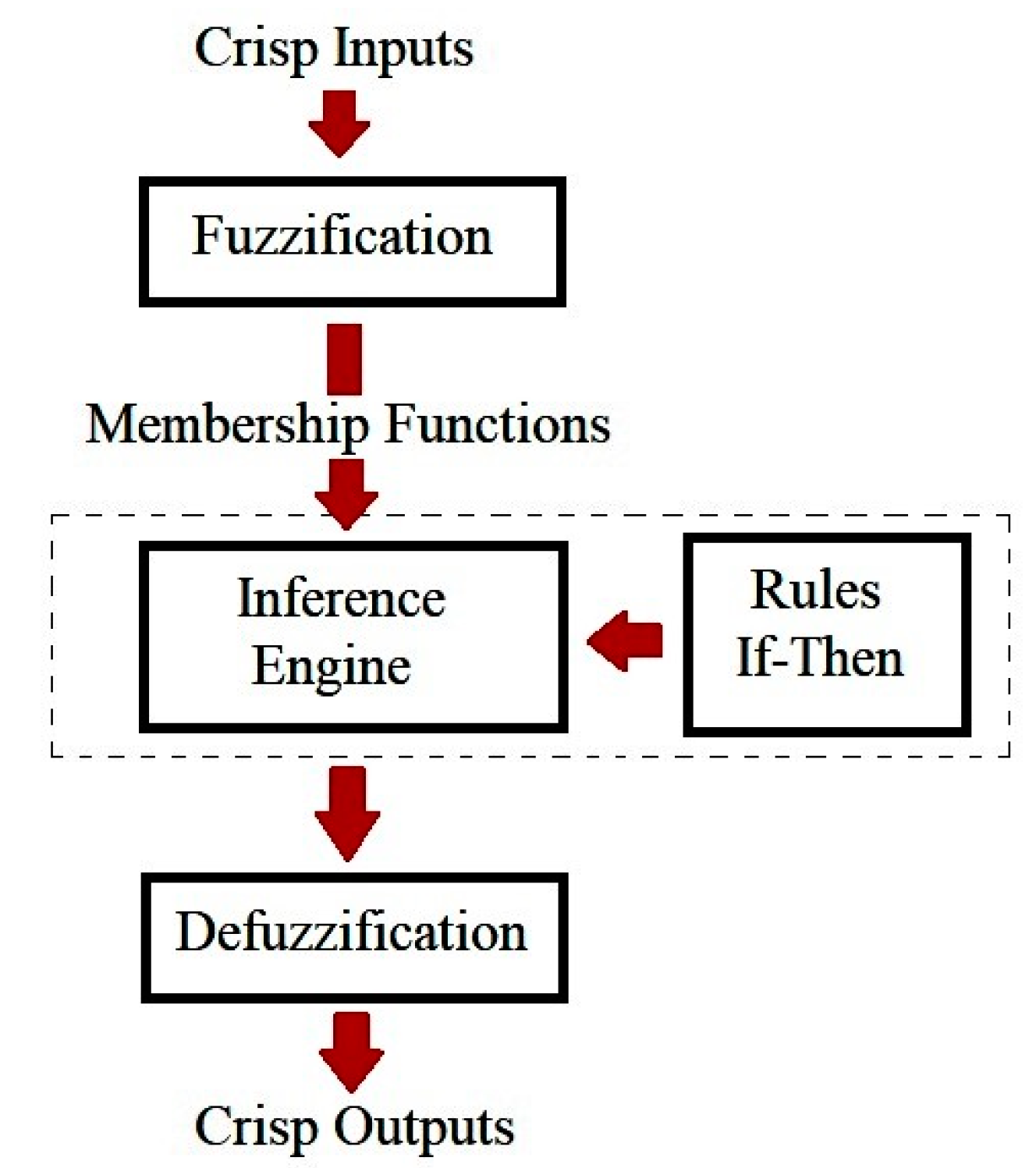
A fuzzy logic control system is developed with the help of four blocks. The first is fuzzification, which converts a crisp input value into a fuzzy value by assigning a degree of membership to the input. Then, the second block is an inference engine that deduces the fuzzy result from fuzzified inputs on the basis of the if–then rules block. The if–then rules is the rule base that contains all the relevant combinations of inputs and outputs that are designed by the user to denote a mathematical relationship between them [
1,
3,
4,
5,
13]. On the basis of membership functions, the fuzzified inputs and outputs are distributed into different sets. The controller provides a crisp output that is derived from the fuzzy output that the inference engine generated. This conversion of inference engine output from fuzzy to crisp is done by the defuzzification process.
Figure 1 shows a general fuzzy-logic-based control system in the form of a block diagram.
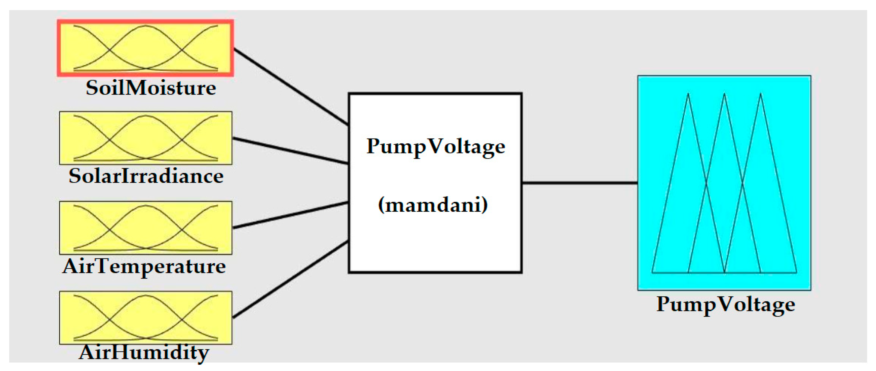
Figure 2 shows the fuzzy inference system developed in MATLAB. Our fuzzy inference system is designed using the MAMDANI approach of fuzzy inference. As a result, the AND operator is realized by calculating the minimum, whereas the OR operator is achieved by calculating the maximum [
3,
13,
14,
15]. Considering the four input variables, soil moisture, solar irradiance, air temperature, and air humidity, the output variable, pump voltage, is controlled based on the fuzzy rules defined in the MATLAB fuzzy rule base.
We chose pump voltage as the output variable because the quantity of water required in the soil can be varied by varying the DC pump’s terminal voltage since the pump speed is directly related to the pump input voltage. To prove that by changing the DC pump’s terminal voltage, the rate of flow of water can be changed; we conducted an experiment in which the pump input voltage is changed manually, and at each voltage value the time needed to fill an empty mug is noted. The experimental data of pump voltage vs. pump water output are shown in
Table 1.
2.1. Membership Functions
Each of the input variables is designed with three membership functions and the output variable with five membership functions [
1,
16]. All input and output variables are defined with the help of trapezoidal and triangular membership functions and linguistic variables [
17,
18]. The triangular membership function and the trapezoidal membership function were implemented solely for the sake of simplicity and for achieving good quality control. According to Lotfi A. Zadeh, the simplest methods work the best because they are intuitively clear and we can easily make use of our intuition and the mathematical formulas together, but if we use complex functions, we can only rely on the formulas as they are difficult to intuitively understand. This explanation is reasonable on the qualitative level and the quantitative explanation is provided in the research [
3,
19].
2.1.1. Soil Moisture
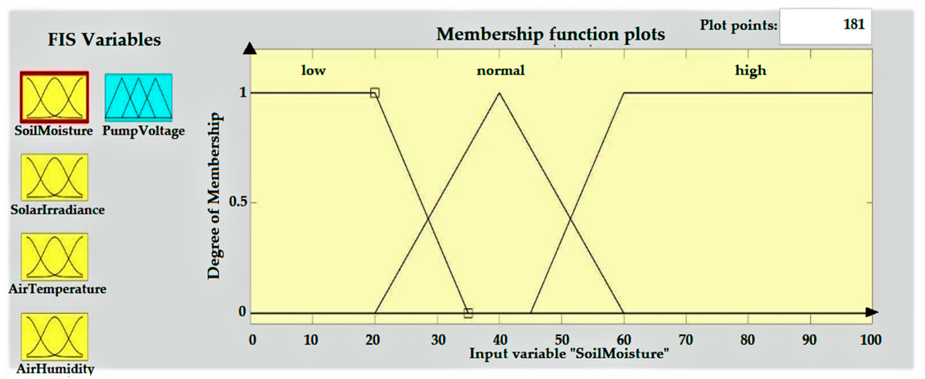
The soil moisture input variable is defined with the help of three linguistic variables, namely low, normal, and high, as shown in
Figure 3. It ranges from 0 to 100 to denote the percentage of moisture content in the soil. The membership function parameters are given below:
Low—trapezoidal membership function with params [−36 −4 20 35]
Normal—triangular membership function with params [20 40 60]
High—trapezoidal membership function with params [45 60 104 136]
2.1.2. Solar Irradiance
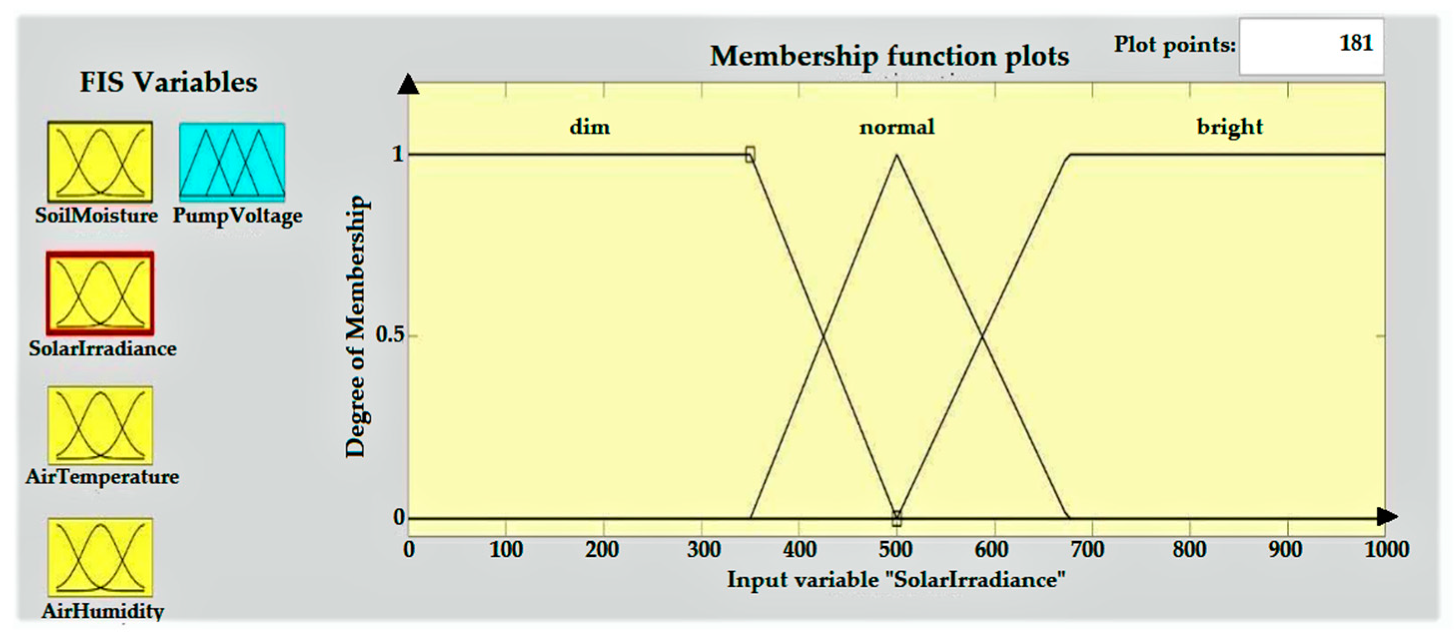
The solar irradiance input variable is defined with the help of three linguistic variables, namely dim, normal, and bright, as shown in
Figure 4. It ranges from 0 to 1000 to denote the amount of solar irradiance incident on the soil w.r.t. watts per square meter. The membership function parameters are given below:
Dim—trapezoidal membership function with params [−360 −40 350 500]
Normal—triangular membership function with params [350 500 675]
Bright—trapezoidal membership function with params [500 675 1040 1360]
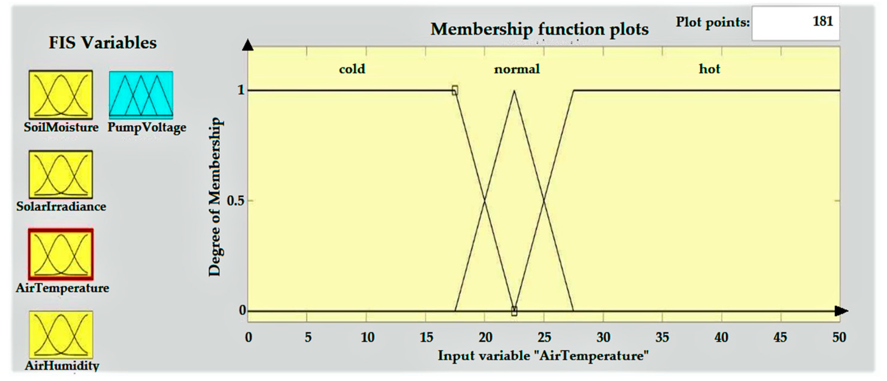
2.1.3. Air Temperature
The air temperature input variable is defined with the help of three linguistic variables, namely cold, normal, and hot, as shown in
Figure 5. It ranges from 0 to 50 to denote the temperature of the air in degrees Celsius. The membership function parameters are given below:
Cold—trapezoidal membership function with params [−18 −2 17.5 22.5]
Normal—triangular membership function with params [17.5 22.5 27.5]
Hot—trapezoidal membership function with params [22.5 27.5 52 68]
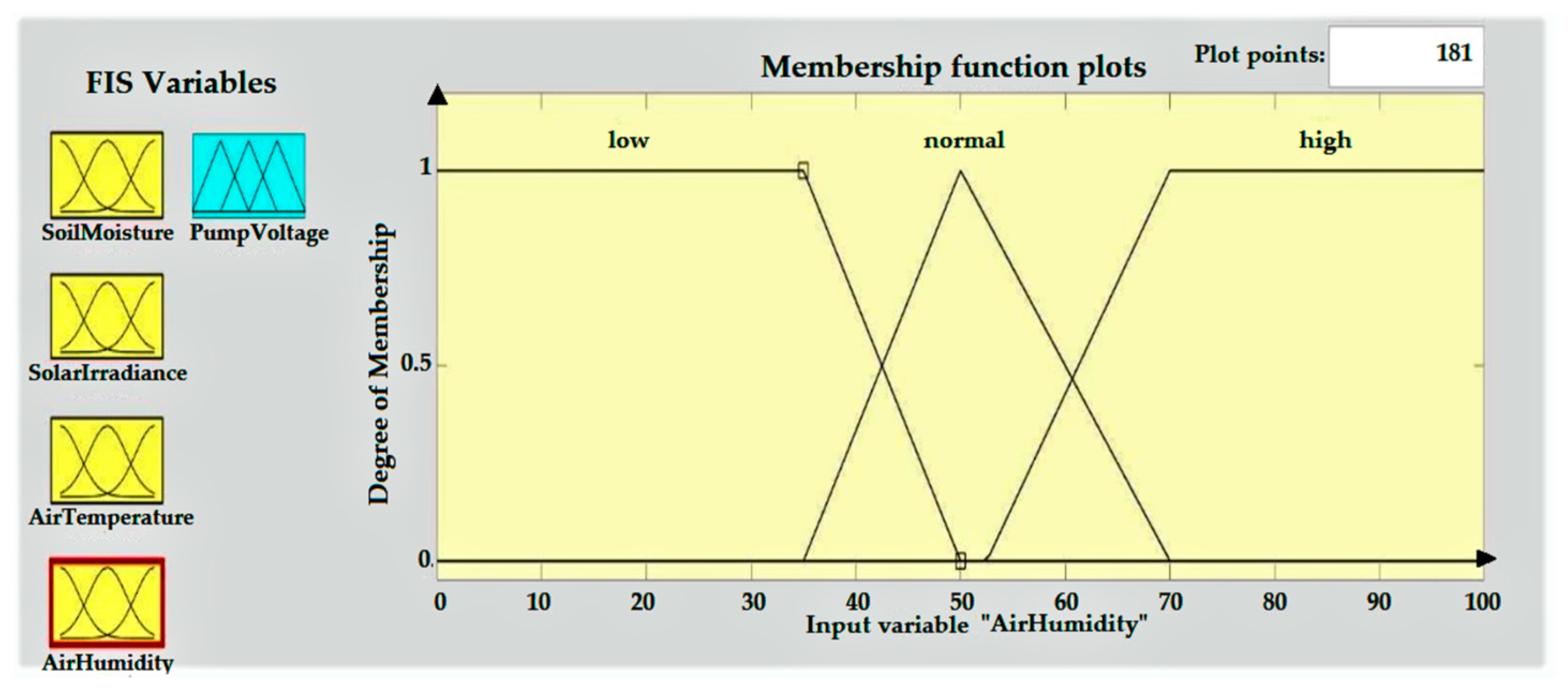
2.1.4. Air Humidity
The air humidity input variable is defined with the help of three linguistic variables, namely low, normal, and high, as shown in
Figure 6. It ranges from 0 to 100 to denote the percentage of moisture content in the air. The membership function parameters are given below:
Low—trapezoidal membership function with params [−36 −4 35 50]
Normal—triangular membership function with params [35 50 70]
High—trapezoidal membership function with params [52.5 70 104 136]
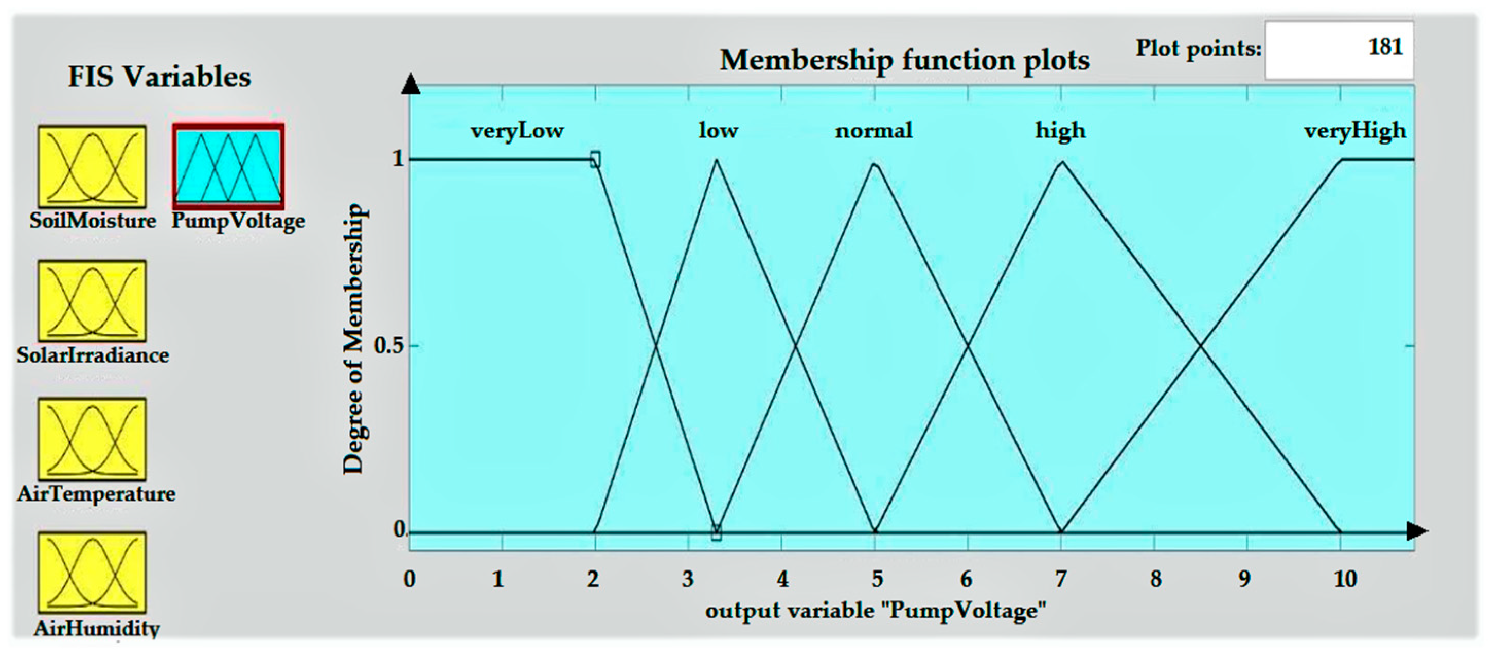
2.1.5. Pump Voltage
The pump voltage output variable is defined with the help of five linguistic variables, namely very low, low, normal, high, and very high, as shown in
Figure 7. It ranges from 0 to 13 to denote the pump voltage in volts. The membership function parameters are given below:
Very low—trapezoidal membership function with params [−2.43 −0.271 2 3.3]
Low—triangular membership function with params [2 3.3 5]
Normal—triangular membership function with params [3.3 5 7]
High—triangular membership function with params [5 7 10]
Very high—trapezoidal membership function with params [7 10 11.1 13.2]
2.2. Fuzzy Rules
Fuzzy rules are defined by taking into consideration how each of the input variables affects the amount of water that the plant needs. First, we check the soil moisture starting from high to low, then solar irradiance is checked starting from dim to bright, then air temperature from cold to hot, and finally air humidity from high to low, as in this sequence we can deduce that if soil moisture is high and solar irradiance is dim and air temperature is cold and air humidity is high then, the need to supply more water to the soil is minimal, and by permuting all the input variables in this order we can say that the water need is increasing, as this is the lowest case. The total count of fuzzy rules that need to be designed can be determined from the general formula for calculating the number of fuzzy rules, which is by multiplying the number of membership functions for each input variable, i.e., 3 × 3 × 3 × 3 = 81 [
1,
13].
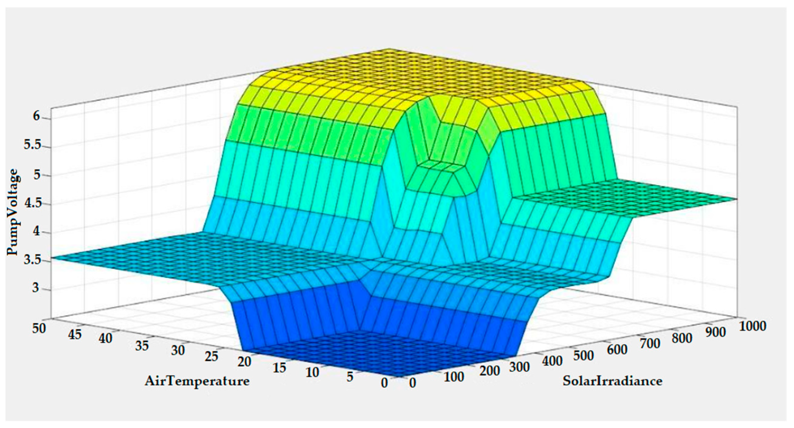
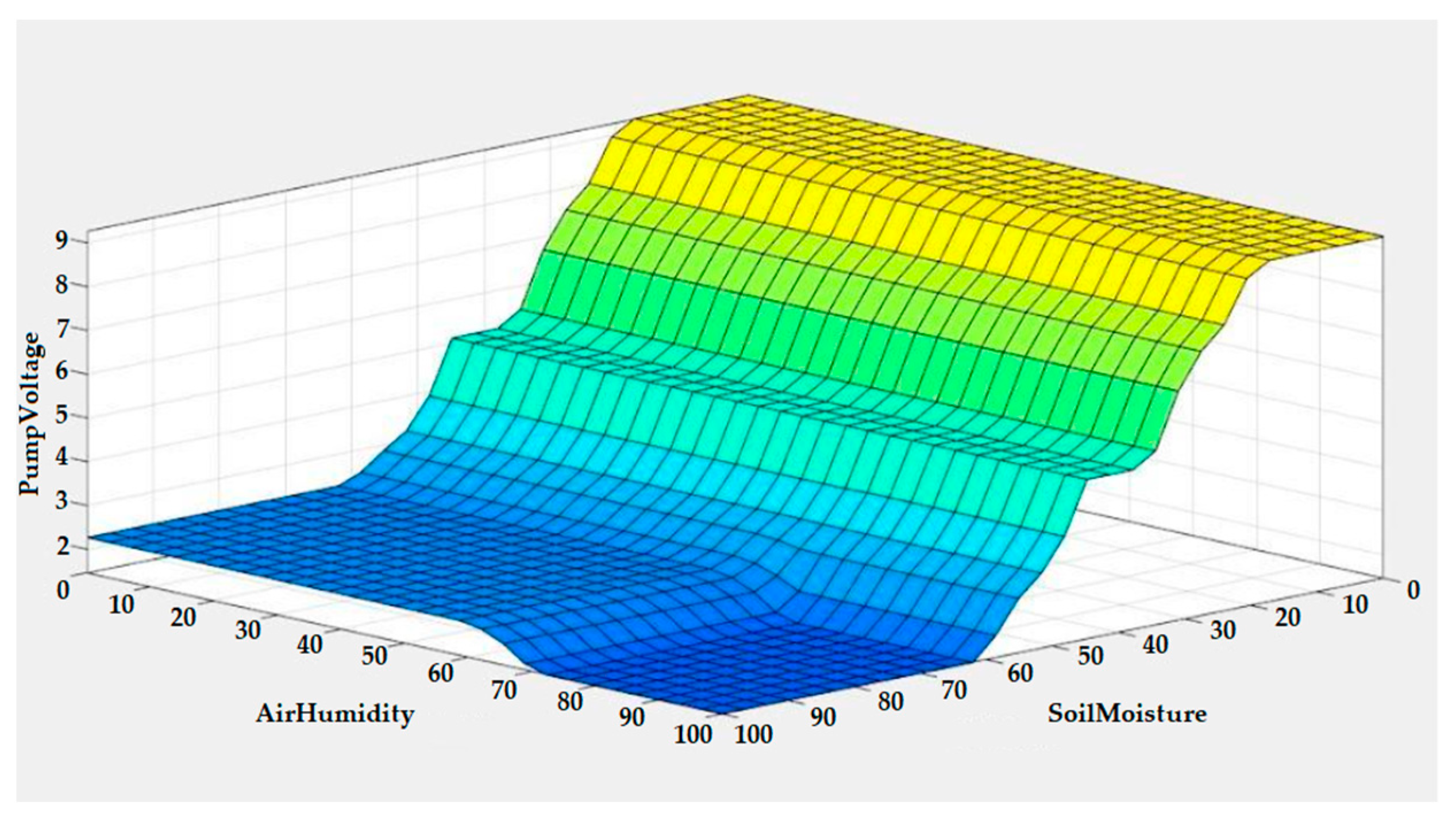
We can verify that the rules defined by the user are correct by viewing the surface graphs automatically generated by the MATLAB software after inputting all the rules, as per the deduction that the amount of water needed by the plant increases directly with solar irradiance and air temperature, while it decreases with increases in soil moisture and air humidity [
13].
We can see that the pump voltage increases with an increase in solar irradiance and air temperature, as shown in
Figure 8, and the pump voltage decreases with an increase in soil moisture and air humidity, as shown in
Figure 9.
3. Verification of Fuzzy Controller
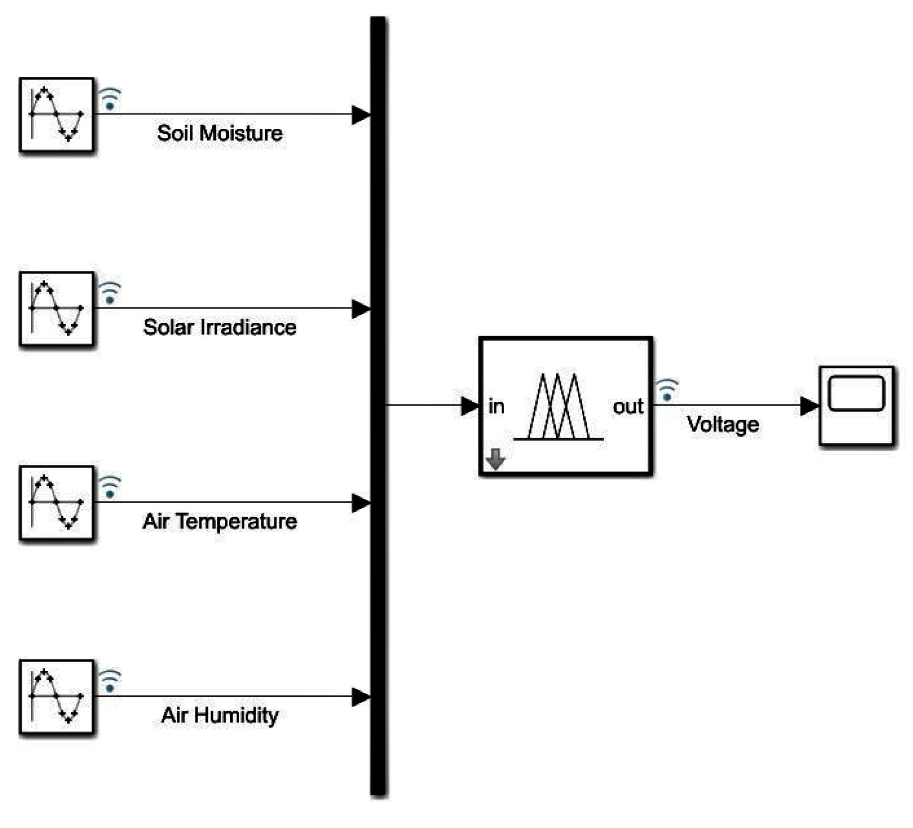
To test the fuzzy controller, we designed a prototype model in Simulink that can be used to test the fuzzy controller for a large set of input values for each input variable.
Figure 10 shows the model used for testing the fuzzy logic controller in Simulink. For each input variable, a sine wave function block is used with different parameters to permute every possibility as defined in the fuzzy rule base. For soil moisture, a sine wave with 50 amplitude and 50 bias is used to get a range of 0–100 as soil moisture will always be in percentage. Solar irradiance is simulated as a sine wave of 500 amplitude and 500 bias to get a range of 0–1000 as solar irradiance can range from 0–1000 watts per meter square. Air temperature is simulated with the help of a sine wave with an amplitude equal to 25 and a bias of 25 to get a range of 0–50, which will be in degrees Celsius, and, finally, the air humidity is the same as soil moisture as it will also be in percent. Each of the waves is specified to engulf each other in all possible ways to get all the permutations of all input variable values.
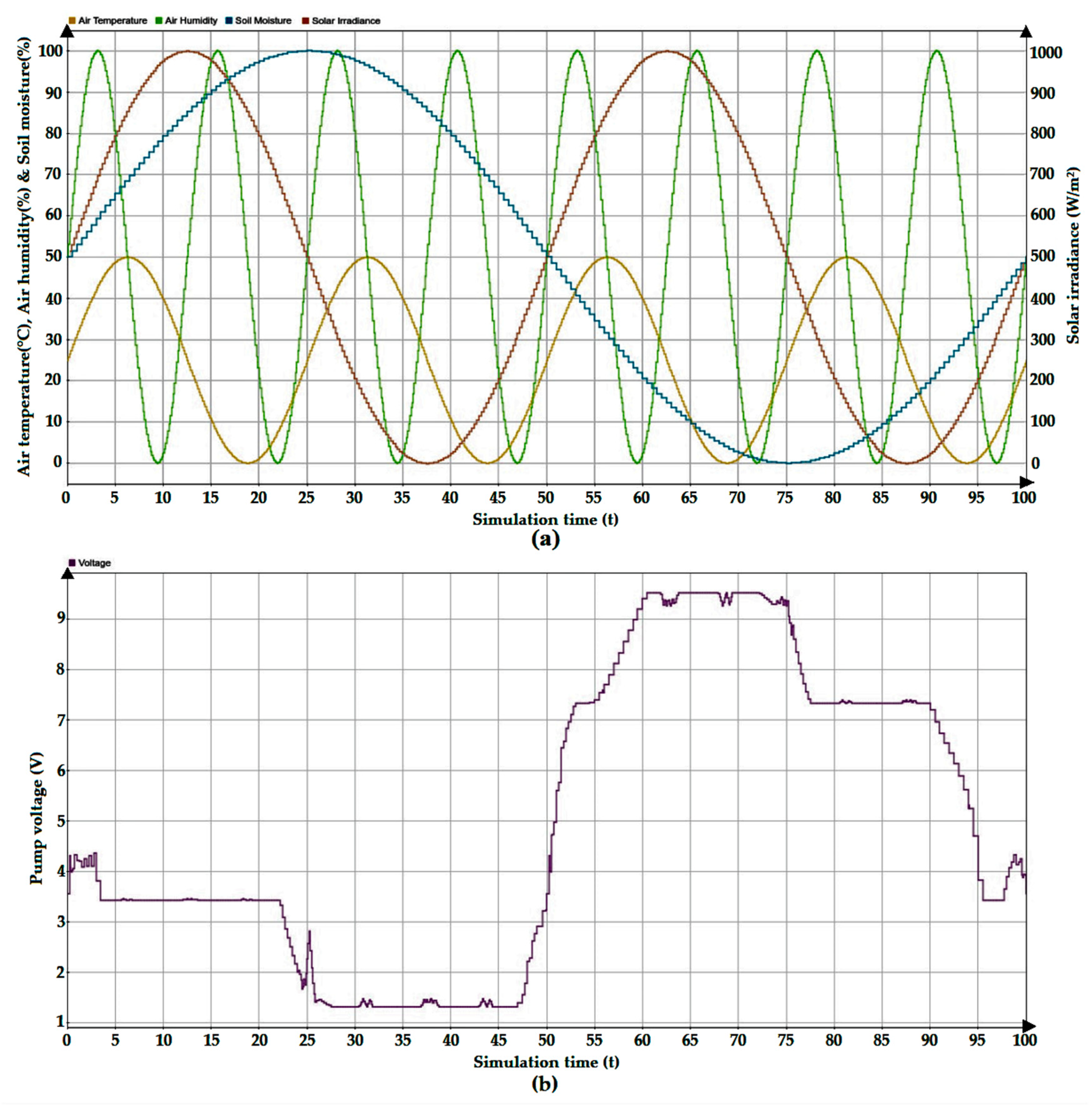
Figure 10 shows the testing model of the system designed in Simulink with the above specifications,
Figure 11a shows the changing values of input variables throughout the simulation, and the pump voltage result is shown in
Figure 11b.
Test Results
According to
Figure 11b for voltage output (simulation time is represented on the x-axis and the value of the respective variable w.r.t. to its unit of measurement is represented on the y-axis), the following observations were made:
While moving from 20 to 30 on the x-axis, we can see that the voltage is decreasing and this happens when solar irradiance is decreasing while soil moisture and air humidity is increasing through the same value. Since soil moisture was almost at the peak and solar irradiance was decreasing, the need for more water was eliminated and pump voltage decreased to minimum.
From 45–60 on the x-axis, we see that the voltage is increasing; this happens while the solar irradiance is also increasing and soil moisture is decreasing. This also suggests that more water is needed when soil moisture is low and solar irradiance is high.
From 75–77, the voltage drops suddenly to around 6.7 volts; as solar irradiance decreases below 400 watts per meter square, soil moisture starts increasing above 0 and air humidity is also increasing. Since there is little sunlight and air humidity is high, the need for water is decreased.
From 90–95, the voltage decreases as soil moisture increases.
From the above observations and
Figure 11, we can clearly see the effect of each input variable on the pump voltage. The pump voltage graph mostly resembles the soil moisture graph but appears inverted, meaning that the soil moisture has the highest impact on the pump voltage, followed by solar irradiance, then air temperature, and lastly air humidity.
4. Analysis of Fuzzy Controller
The fuzzy logic controller was designed with respect to controlling the soil moisture content based on the instantaneous values of the pre-defined input variables that are soil moisture, solar irradiance, air temperature, and air humidity. The pump voltage was chosen as the output variable of the fuzzy controller because of the relationship between pump voltage and the flow rate of water, controlling which is the main purpose of our controller. Since the DC pump that was taken could be easily controlled by changing the terminal voltage and thus changing its speed. Using the observations from the experiment described above and in
Table 1, the following mathematical equations can be written. Since an increase in input voltage results in less time needed to fill the mug completely, we can say that input voltage is inversely proportional to the time needed to fill the mug completely and can be written in mathematical form as:
and the rate of flow of water can be defined by:
Rate of flow of water = change in volume/time taken to fill 500 mL = (500 − 0)/time taken to fill 500 mL,
The above equation can be rewritten as:
From Equations (1) and (2), we can say that the rate of flow of water is directly proportional to the input voltage of the DC water pump.
Mathematically, the relationship between the input variables that are soil moisture, solar irradiance, air temperature, and air humidity and the pump voltage output variable can be defined by:
These four equations can be proved by considering the effect of each input variable on the soil moisture content:
- 1.
Equation (4) is a general equation considering that increasing soil moisture content indicates less need for water and, thus, the inverse relationship between the variable soil moisture and pump voltage;
- 2.
When the value of the solar irradiance increases, it increases the rate of evaporation, and, thus, to maintain the moisture content of the soil, the rate of flow of water from the pump needs to be increased, and, thus, the pump voltage is increased;
- 3.
Air temperature acts similarly as solar irradiance acts upon the moisture content of the soil and, thus, the direct relationship is formed;
- 4.
Air humidity is defined by the inverse relationship because when the moisture content of the air is low the evaporation rate of water in the soil is increased as the dry air tends to absorb the moisture from the surface.
Equation (8) represents the mathematical model of the system.
4.1. System Response w.r.t Each Input Variable
The response of the fuzzy controller with respect to each input variable is analyzed in the same way the above results are found. A test model is designed for each input variable such as soil moisture, solar irradiance, air temperature, and air humidity. Each model is run three times by considering the values of the remaining variables as:
- 1.
Minimum water needed;
- 2.
Maximum water needed;
- 3.
At standard operating conditions.
4.1.1. Soil Moisture
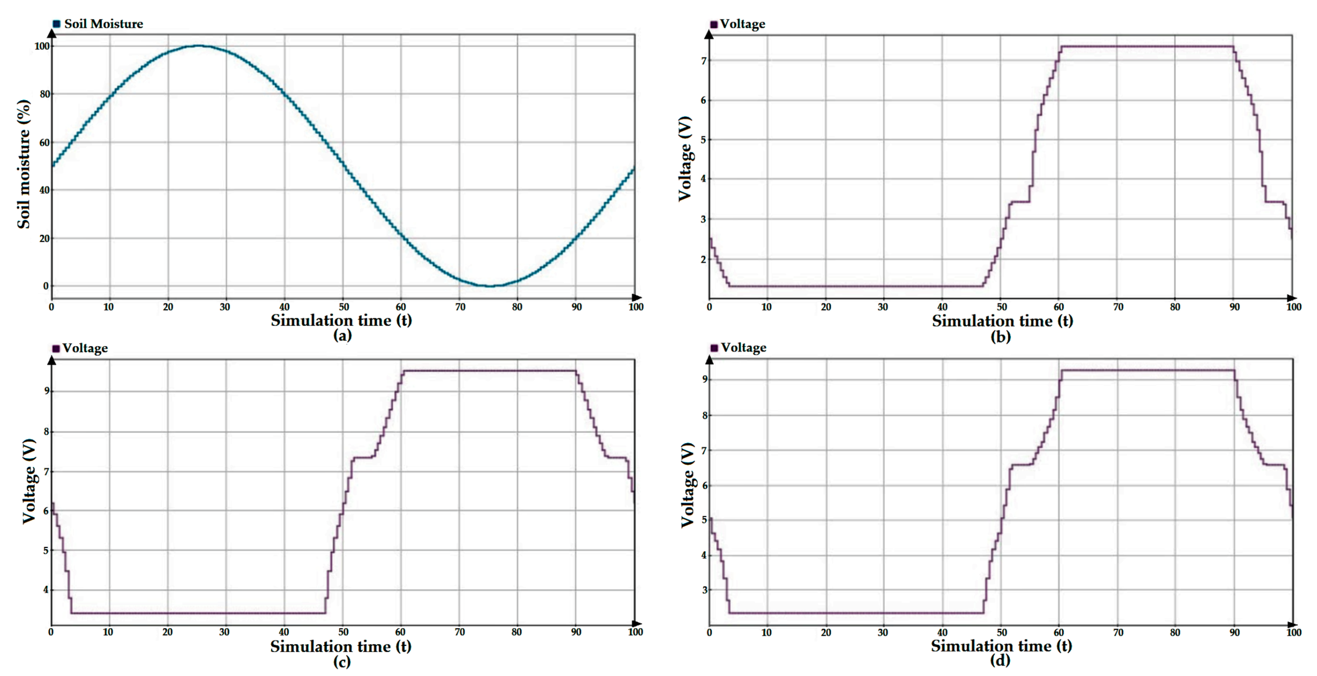
According to Equation (4), the effect of soil moisture on the pump voltage should be inversely proportional, and with an increase in the soil moisture value, the pump voltage should be decreased. This can be validated by the following graphs.
Figure 12a,b show the graphs of soil moisture vs. time and voltage vs. time when all the other variables’ need for water is at a minimum, respectively. When soil moisture is 0–20, we can see that the pump voltage is constant (around 7.3 V). As the soil moisture value increases from 21 to 60, the pump voltage is decreased simultaneously to somewhere around 1 V and then is maintained there as the soil moisture increases further to 100 and back to 60.
As soon as the soil moisture starts decreasing below 60, the pump voltage is increased gradually to 7.3 V. The pump’s voltage is not increased above 7.3 V because the need for water is at minimum by the other variables such as solar irradiance and air temperature being set to minimum and the air humidity being set to maximum, signifying no effect of these variables on the evaporation rate of water from the soil. This is with respect to the fuzzy controller only and when the hardware model is connected to it the output will change significantly as the minimum voltage our system can work on is 3.3 V. So, as soon as the fuzzy controller outputs a value below 3.3, the actual value becomes 0 and the DC pump is shut down.
Similarly, considering that the need for water is at maximum w.r.t. to the other variables, the effect of soil moisture on the pump voltage is defined by the graph shown in
Figure 12c, Considering the soil moisture value from
Figure 12a. We can see that the range of pump voltage has shifted from 1–7.3 V to 3.2–9.5 V, but it is still in accordance with our Equation (7) as the voltage is increased when soil moisture decreases from 60–20 and vice versa. The range of pump voltage has changed slightly from 3.2–9.5 V to 2.2–9.2 V at standard operating conditions, according to
Figure 12d considering soil moisture value from
Figure 12a. To get the graph at standard operating conditions, we manually set solar irradiance to 600.00 W/m², air temperature to 25 °C, and air humidity to 50%. This slight decrease in the range is due to a decrease in the solar irradiance value from 1000.00 W/m² at max to 600.00 W/m², while the graph is almost identical.
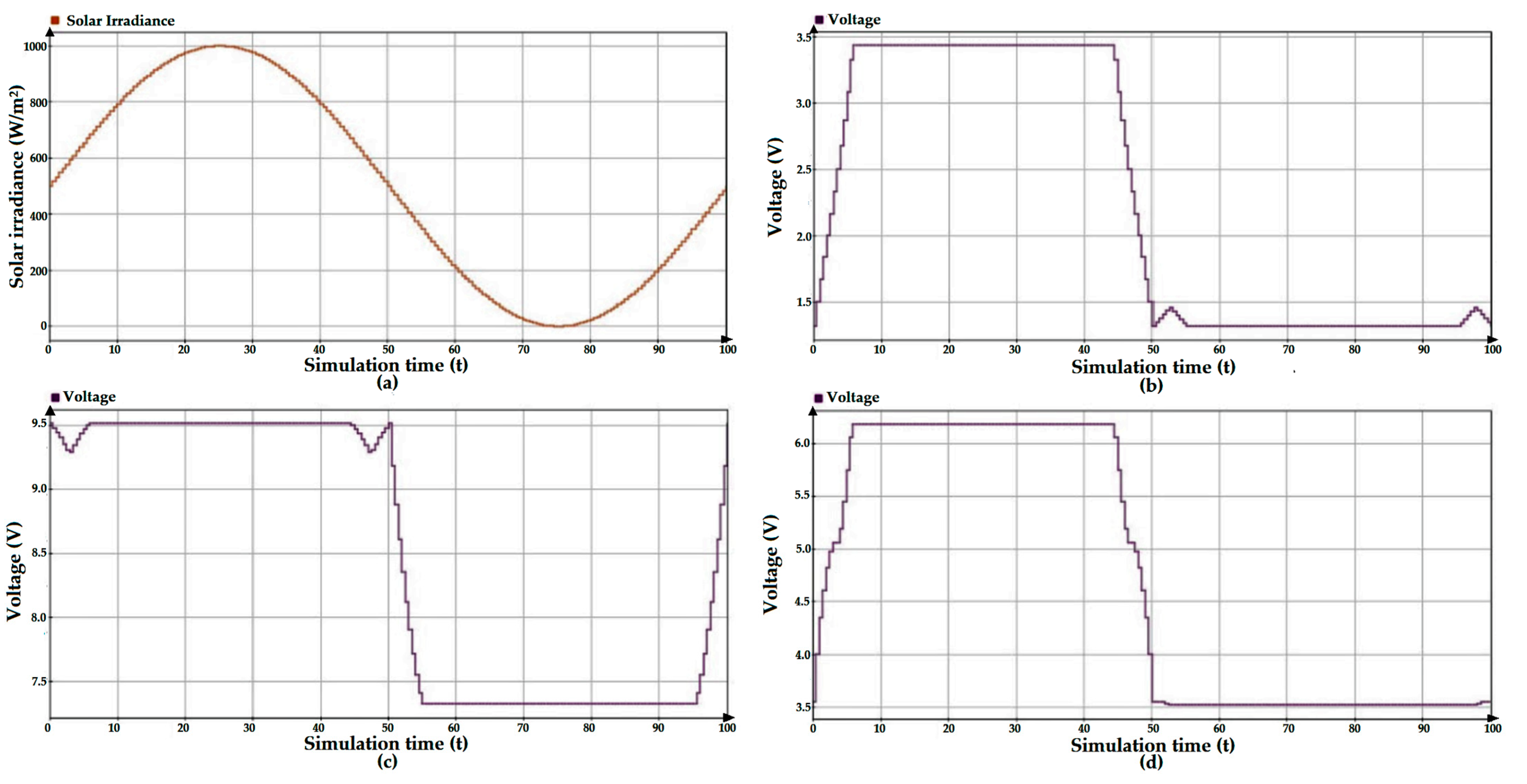
4.1.2. Solar Irradiance
According to Equation (5), the effect of solar irradiance on the pump voltage should be directly proportional, and with an increase in the soil moisture value the pump voltage should also be increased [
8]. This can be validated by the following graphs shown in
Figure 13.
Figure 13a,b show the graphs of solar irradiance vs. time and voltage vs. time, respectively, when all the other variables’ need for water is at a minimum. When solar irradiance is 0 to 400.00 W/m², we can see that the pump voltage is constant (around 1.35 V). As the solar irradiance value increases from 400.00 W/m² to 700.00 W/m², the pump voltage is increased simultaneously to somewhere around 3.4 V and then is maintained there as the solar irradiance increases further to 1000.00 W/m² and back to 700.00 W/m². As soon as the solar irradiance starts decreasing below 700.00 W/m², the pump voltage is decreased gradually to 1.35 V. The pump’s voltage is not increased above 3.4 V because the need for water is at minimum by the other variables such as air temperature being set to minimum and the air humidity and soil moisture being set to maximum, signifying no effect of these variables on the evaporation rate of water from the soil.
Similarly, considering that the need for water is at maximum w.r.t. to the other variables, the effect of solar irradiance on the pump voltage is defined by the graph shown in
Figure 13c, Considering solar irradiance value from
Figure 13a. We can see that the range of the pump voltage has shifted from 1.35–3.4 V to 7.25–9.5 V, and it is still in accordance with our Equation (5), as the voltage is increased when solar irradiance increases from 300.00–500.00 W/m² and vice versa. The range of the pump voltage is changed slightly from 7.25–9.5 V to 3.5–6.25 V at standard operating conditions, according to
Figure 13d, Considering the solar irradiance value from
Figure 13a. To get the graph at standard operating conditions, we manually set soil moisture to 50%, air temperature to 25 °C, and air humidity to 50%. This slight decrease in the range is due to a decrease in solar irradiance value from 1000.00 W/m² at max to 600.00 W/m², while the graph is almost identical.
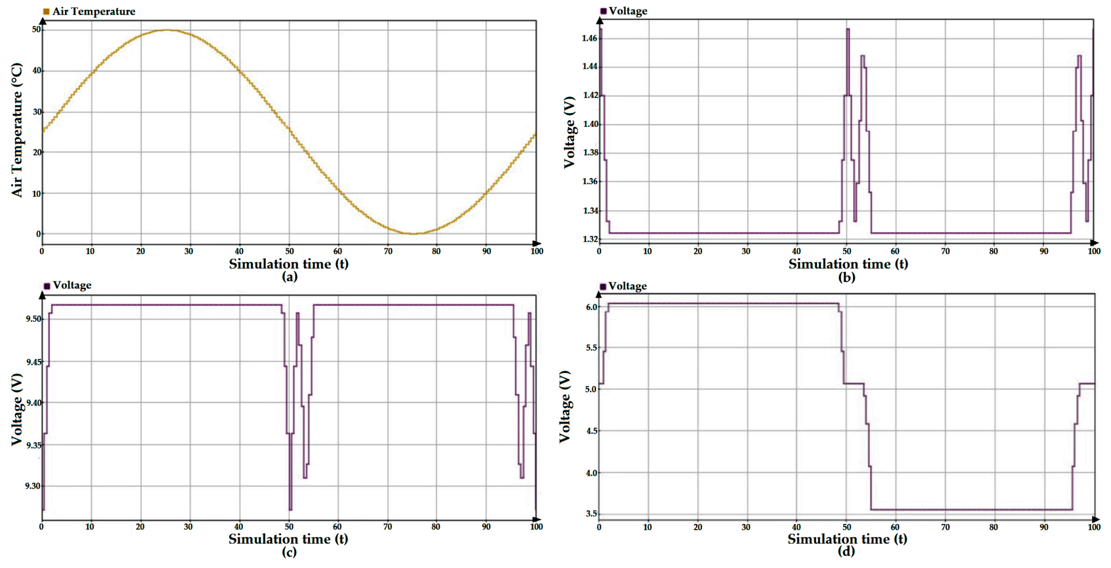
4.1.3. Air Temperature
According to Equation (6), the effect of air temperature on the pump voltage should be directly proportional, and with an increase in the air temperature value the pump voltage should also be increased [
8]. This can be validated by the following graphs shown in
Figure 14.
In
Figure 14b, when the need for water is minimum because of other factors, then the effect of air temperature can be neglected as the value of pump voltage is below 3.3 V and the Arduino microcontroller will set the voltage to 0 V when below this level. Similarly, considering that the need for water is at maximum w.r.t. to the other variables, the effect of air temperature on the pump voltage is still negligible, as shown by the graph in
Figure 14c.
From
Figure 14d, we can see that the pump voltage changes according to Equation (6). The effect of air temperature is observed in standard conditions. To get the graph at the standard operating conditions we manually set solar irradiance to 600.00 W/m², soil moisture to 50 °C, and air humidity to 50%. The graph depicts a range of 3.6–6.1 V, while between the range, the pump voltage is seen to be increasing when the air temperature increases above 15 degrees Celsius and hits the maximum when the air temperature reaches 27 degrees Celsius. Since between the range, the pump voltage increases with an increase in air temperature, and Equation (6) is validated.
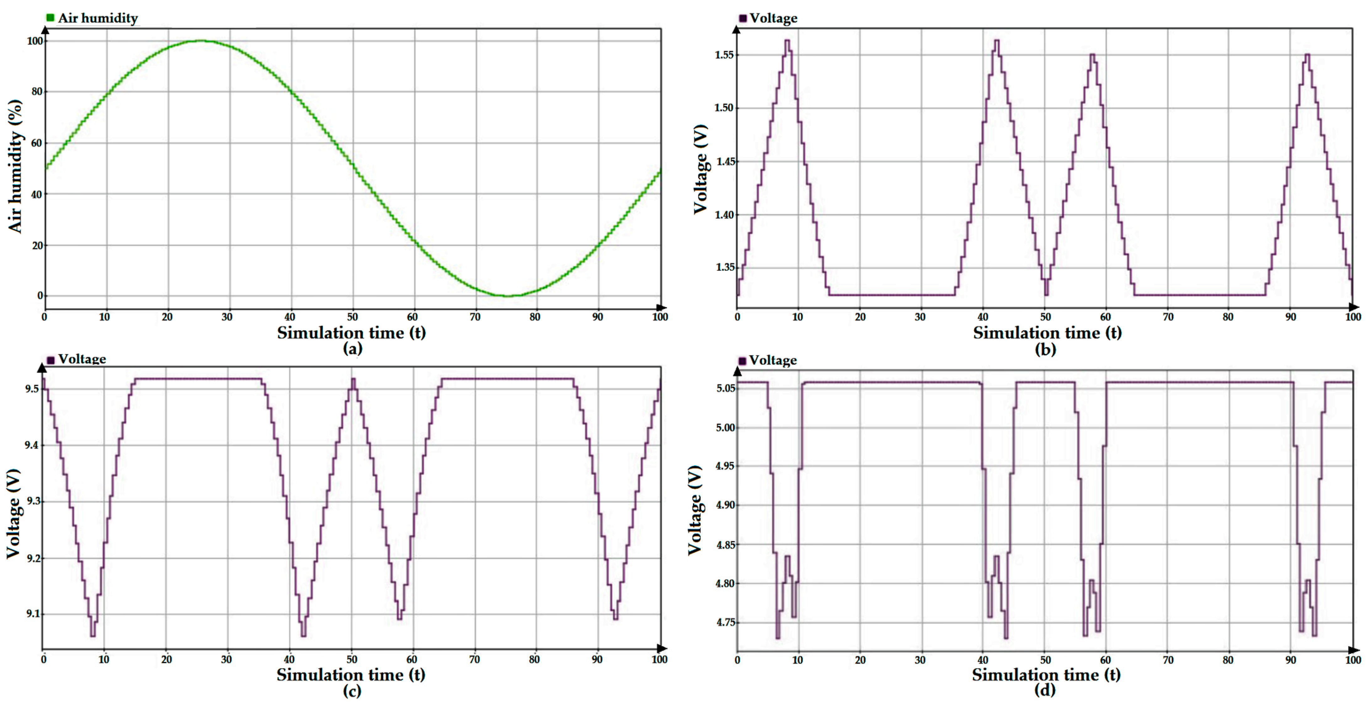
4.1.4. Air Humidity
According to Equation (7), the effect of air humidity on the pump voltage should be inversely proportional, and with an increase in the air humidity value the pump voltage should be decreased [
8]. This can be validated by the following graphs shown in
Figure 15.
Figure 15a,b show the graphs of air humidity vs. time and voltage vs. time, respectively, when all the other variables’ need for water is at a minimum. This graph can be neglected as the maximum voltage observed is less than 3.3 V. Similarly, considering that the need for water is at maximum w.r.t. to the other variables, the effect of air humidity on the pump voltage is defined by the graph shown in
Figure 15c. This graph also does not provide enough information as the range observed is only 0.4 V and, based on our hardware resolution, it will be rounded off. From
Figure 15d, we again observed that the graph lies between an overall range of 0.3 V and the actual output will be rounded off. This concludes that the effect of air humidity is negligible on the pump voltage.
The highest range observed from the above graphs was the effect of soil moisture on pump voltage and the second highest was solar irradiance. The effect of air temperature and air humidity is found to be negligible, while the graph of air temperature under standard conditions showed some response. We can conclude that the highest priority was given to soil moisture as it is also the control variable that we need to monitor, and then the second is solar irradiance as it is the largest factor that affects the amount of water needed by the soil, and the third and fourth are air temperature and air humidity, respectively. We can say that the system is highly sensitive to change in soil moisture and then moderately sensitive to change in solar irradiance, less sensitive to change in air temperature, and minutely sensitive to change in air humidity.
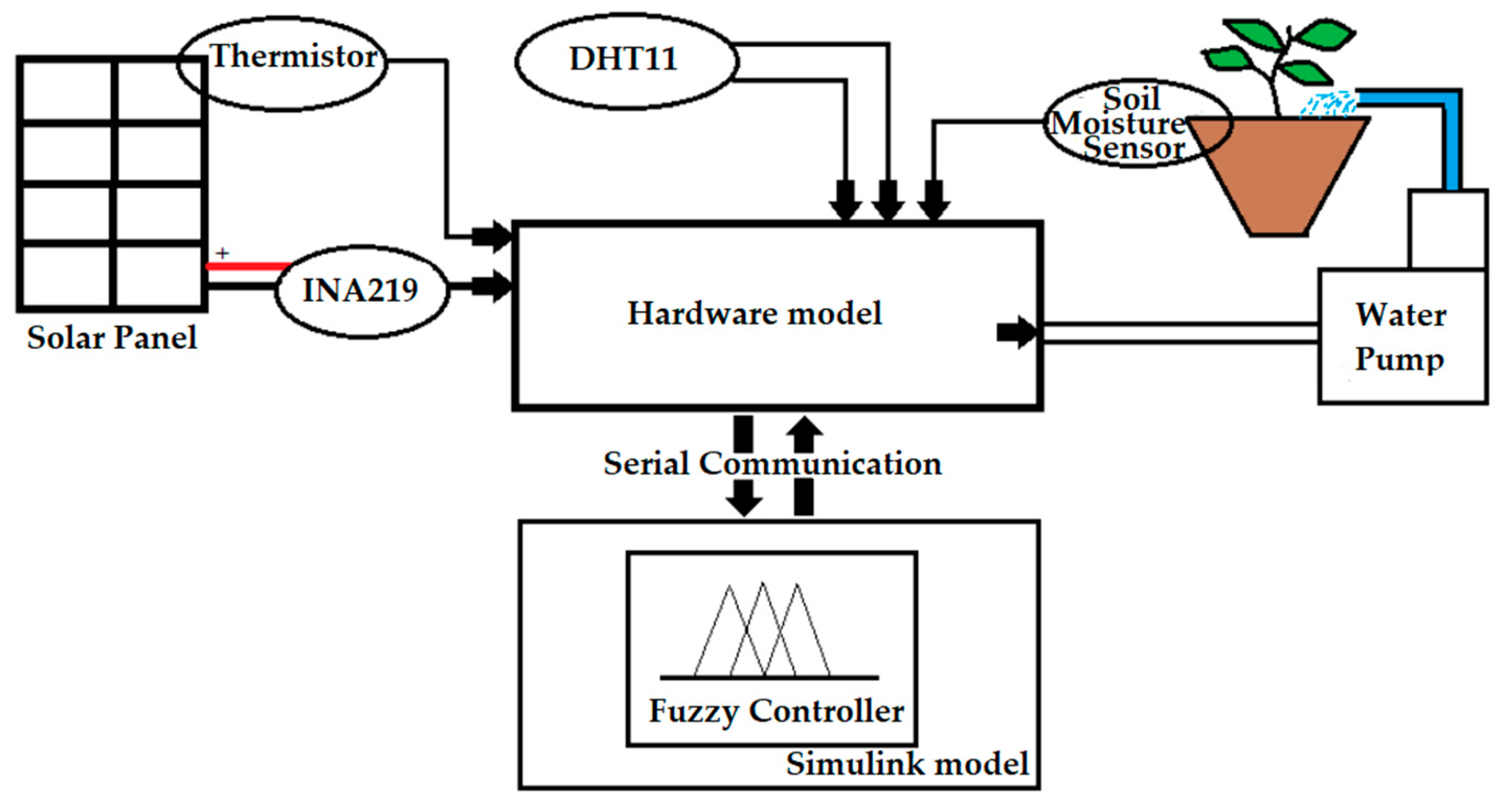
5. Proposed Model
For data acquisition, the Arduino microcontroller is used with different types of sensors to collect the real-time readings of all the input variables. Arduino Nano is used for the base of our system. Serial communication is established between Arduino and Simulink to get all the input values and the output is then sent back to Arduino, which also controls the input voltage of the pump [
2,
20,
21,
22,
23,
24].
Figure 16 shows all the relevant components and their connectivity in the proposed model in the form of a block diagram.
Soil moisture is taken in by soil moisture sensor RC-A-4079, which comprises a probe with two electrodes and one eight-pin integrated circuit. The two electrodes on the probe act as a resistor with variable resistance (just like a potentiometer). The resistance of these two electrodes changes relative to the quantity of water in the soil. The sensor determines the soil moisture level by applying a voltage to the resistance and measuring the voltage drop from the source [
2,
23,
25,
26,
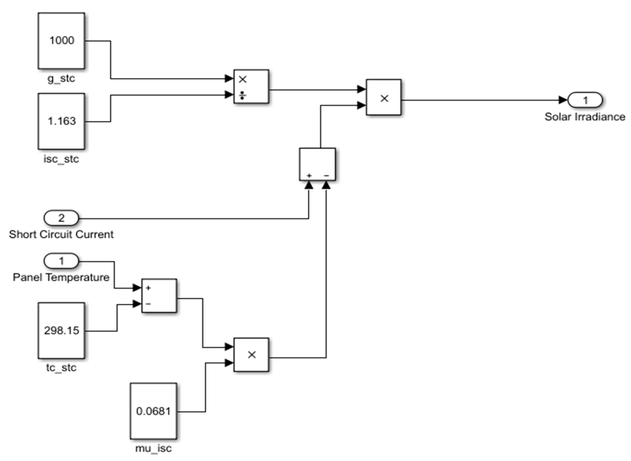
27]. Solar irradiance is calculated by using solar panel characteristics as described in [
28]; short-circuit current and solar panel temperature are substituted in the formula:
where
GIsc = the solar irradiance calculated using the short-circuit current,
GSTC = the solar radiation in standard operating conditions = 1000 W/m²,
I
SCstc = the short-circuit current in standard conditions (
Appendix A),
ISC = the short-circuit current read from the sensor,
μ
Isc = the temperature coefficient for the short-circuit current (
Appendix A),
TC = the measured temperature of the solar panel,
TCstc = the temperature of the solar panel at STC (298.15 K).
The short-circuit current of the solar panel is measured by short-circuiting the solar panel terminals using a 5 V DC relay and then taking the current value from an INA219 current sensor and the panel temperature from a thermistor attached to the solar panel [
29,
30,
31,
32,
33,
34]. Air temperature and air humidity are taken from a DHT11 sensor [
23,
26].
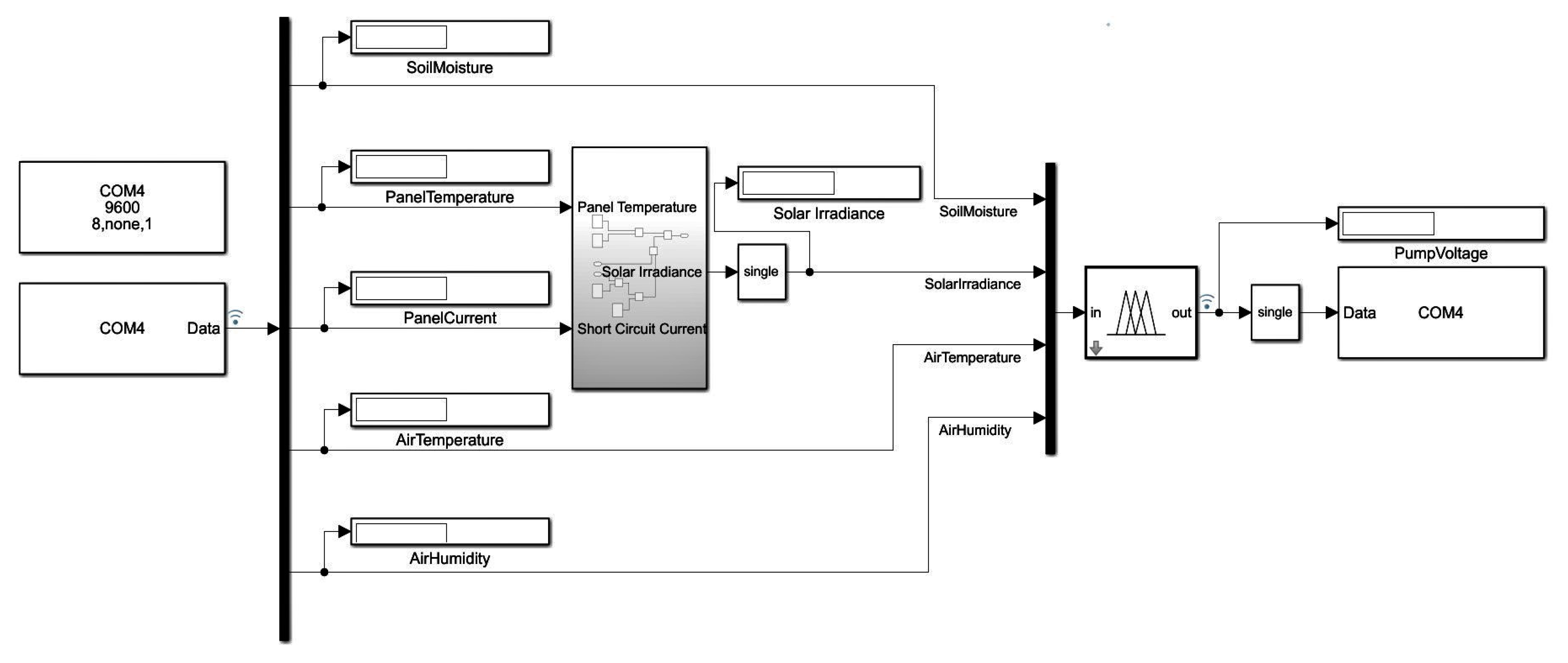
All the values from the sensors are taken in by the Arduino and then sent to the Simulink model (block parameters can be found in
Appendix A), as shown in
Figure 17, with a serial receive block; solar irradiance is calculated by passing the panel temperature and short-circuit current through a subsystem block, which comprises the logic to find the solar irradiance value, as shown in
Figure 18; input variables are passed to the fuzzy controller block and the output is then sent to the Arduino using the serial send block. The Arduino then changes the input voltage of the DC water pump using the PWM technique and motor driver [
6,
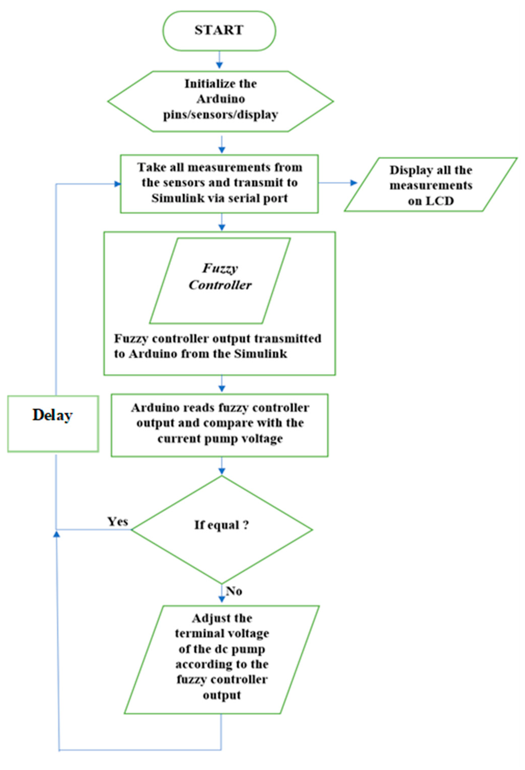
35]. After changing the voltage of the DC water pump, a delay is programmed into the Arduino to wait for 10 minutes and start again. All of these steps can be summarized by the flow chart defined in
Figure 19. The flow chart does not have a stop block because the algorithm is designed to work recursively and keeps on repeating the process of gathering sensor data and changing the speed of the water pump based on them. The algorithm and the system were developed after extensive research to work efficiently based on all the input factors and sensor modules [
7,
10,
11,
12,
24,
27,
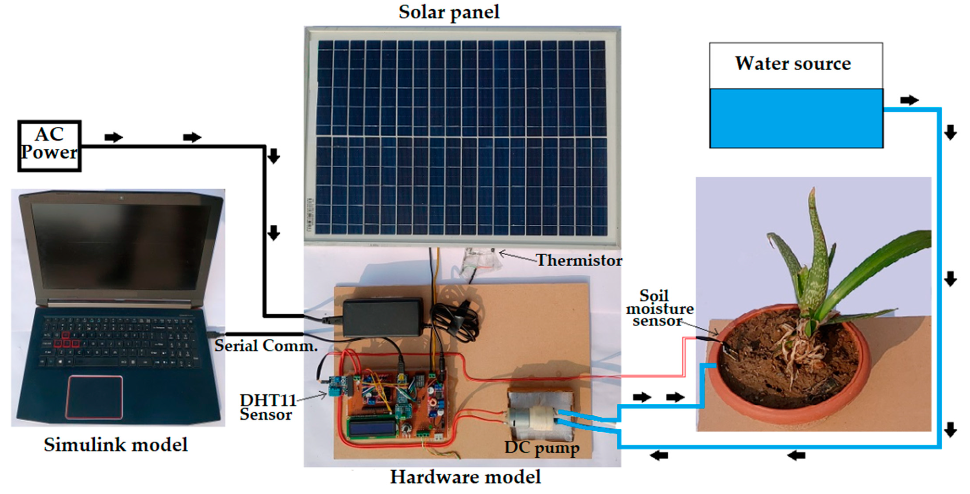
36]. The final working model of the system is shown in
Figure 20.
6. Results
The automatic irrigation control system is operated at different times during the day from sunrise to before sunset on different days to obtain different input values from various sensors to observe the change in output voltage and the pump’s water flow rate. The results obtained are shown in
Table 2.
According to
Table 2, we observed that the input voltage of the water pump increases based on the environmental values measured from the various sensors. We can see that when soil moisture is measured to be 0% and 4%, the solar intensity ranges from 545.68 W/m² to 662.61 W/m², the air temperature is approximately equal, which is 22.7 degrees Celsius, and the air humidity is 57%. This results in the fuzzy logic controller giving the output of 9.36 V and 8.93 V, both of them being near 9 V, which is in the maximum range of our system, providing the most water to the plant. As the soil moisture value increases to 22% and there is a significant solar intensity of 330.76 W/m² and the air temperature increases to 29.74 degrees Celsius and the air humidity is decreased to 37%, then the fuzzy controller gives the output of 7.24 V, reducing the pump’s voltage from before when there was no moisture in the soil.
We saw that the minimum voltage observed during the day was 1.85 V when soil moisture was around 84% with a solar intensity of around 528.21 W/m² and the air temperature being 21.1 degrees Celsius and air humidity equaling 60%, Our system cannot modulate the voltage to below 3.3 V, so it turns the pump off at this range indicating 0 V. At soil moisture of 84% and 85%, we can see the solar irradiance values at 528.21 W/m² and 628.72 W/m², respectively. We can ignore the changes in air temperature and humidity as they are much less. We saw that the fuzzy controller output changed from 1.85 V to 2.73 V because of the increase in the value of solar irradiance. Now, when the soil moisture is further increased to 90%, the value of solar irradiance is 673.42 W/m², while comparing this with the values of other variables at a soil moisture level of 85%, we saw a further increase in the solar irradiance value, a 3.79-degree increase in air temperature, and a 6% decrease in air humidity—all variables indicating more need for water. Thus, the fuzzy controller output can be seen increasing to 3.4 V and the actual pump is switched ON. The circuit diagram, the Arduino program and other
supplementary materials can be downloaded from github (link to github repository is mentioned in the
supplementary materials section below).
7. Conclusions
The automatic control system was developed using the fuzzy logic controller, which is able to handle different values and to run and control the DC water pump’s input voltage based on environmental factors like soil moisture, solar irradiance, air temperature, and air humidity. By controlling the water flow rate, thereby controlling the soil moisture and taking it as an input parameter, a closed-loop control system that is getting continuous feedback is formed. This, in turn, saves water when sufficient moisture is present in the soil and it is not required; also, the plant/crop is not overwatered and is provided with only the sufficient amount of water that is required for optimal growth. The sufficient amount required by the plant/crop is always dependent on the type of plant/crop and the type of soil, and thus the pump voltage membership function values needs to be tweaked for different types of plant/crop and soil. By automating the irrigation process, we also achieved the prevention of under-watering of the plant/crop since the system would automatically provide water to the plant/crop when it senses the need depending upon the soil moisture and the various environmental factors incorporated in the system through different sensors. In addition, our system uses solar panel characteristics to measure the solar irradiance instead of using a pyranometer, which is expensive, or using commonly available radiation sensors, which are not suitable to capture the radiation for the whole spectrum. This solar irradiance measurement not only provides us with a better precision while measuring solar irradiance but also reduces the cost of the system.
Author Contributions
All authors planned the study, contributed to the idea and field of information; conceptualization, T.T. and A.K.S.; investigation, A.K.S.; methodology, T.T. and A.K.S.; project administration, A.K.S., M.F.A., G.S., P.N.B. and T.S.; software, T.T.; analysis, A.K.S., T.T., M.F.A. and G.S.; resources, T.T.; conclusion, A.K.S. and T.T.; writing—original draft preparation, T.T.; writing—review and editing, A.K.S., T.T., M.F.A. and G.S.; validation, A.K.S. and G.S.; visualization, T.T.; supervision, A.K.S. and P.N.B. All authors have read and agreed to the published version of the manuscript.
Funding
This research received no external funding.
Data Availability Statement
Not applicable here.
Conflicts of Interest
The authors declare no conflict of interest.
Appendix A
| Solar panel specifications |
| ISCstc | 1.163 A |
| μIsc | 0.0681 AK−1 |
| Simulink serial configuration block parameters |
| Baud rate | 9600 bps |
| Data bits | 8 |
| Parity | None |
| Stop bits | 1 |
| Byte order | little-endian |
| Flow control | None |
| Timeout | 10 |
| Simulink serial receive block parameters |
| Terminator | CR/LF |
| Data size | [1 5] |
| Data type | Single |
| Block sample time | 0.01 |
| Simulink serial send block parameters |
| Terminator | CR/LF |
References
- Khatri, V. Application of Fuzzy logic in water irrigation system. Int. Res. J. Eng. Technol. 2018, 5, 3372. [Google Scholar]
- Akter, S.; Mahanta, P.; Mim, M.H.; Hasan, M.R.; Ahmed, R.U.; Billah, M.M. Developing a smart irrigation system using arduino. Int. J. Res. Stud. Sci. Eng. Technol. 2018, 6, 31–39. [Google Scholar]
- Espitia, H.; Soriano, J.; Machón, I.; López, H. Design methodology for the implementation of fuzzy inference systems based on boolean relations. Electronics 2019, 8, 1243. [Google Scholar] [CrossRef]
- Wang, L.X. A Course in Fuzzy Systems and Control; Prentice-Hall, Inc.: Hoboken, NJ, USA, 1996; Available online: https://dl.acm.org/doi/abs/10.5555/248374 (accessed on 22 August 2022).
- Li, J.; Gong, Z. SISO Intuitionistic Fuzzy Systems: IF-t-Norm, IF-R-Implication, and Universal Approximators. IEEE Access 2019, 7, 70265–70278. [Google Scholar] [CrossRef]
- Petru, L.; Mazen, G. PWM control of a DC motor used to drive a conveyor belt. Procedia Eng. 2015, 100, 299–304. [Google Scholar] [CrossRef]
- Debo-Saiye, Y.; Okeke, H.S.; Mbamaluikem, P.O. Implementation of an Arduino-Based Smart Drip Irrigation System. Int. J. Trend Sci. Res. Dev. 2020, 5, 1130–1133. [Google Scholar]
- Sheikh, S.S.; Javed, A.; Anas, M.; Ahmed, F. Solar based smart irrigation system using PID controller. IOP Conf. Ser. Mater. Sci. Eng. 2018, 414, 012040. [Google Scholar] [CrossRef]
- Rajeshkumar, N.; Vaishnavi, B.; Saraniya, K.; Surabhi, C. Smart crop field monitoring and automation irrigation system using IoT. Int. Res. J. Eng. Technol. 2019, 6, 7976–7979. [Google Scholar]
- Vij, A.; Vijendra, S.; Jain, A.; Bajaj, S.; Bassi, A.; Sharma, A. IoT and machine learning approaches for automation of farm irrigation system. Procedia Comput. Sci. 2020, 167, 1250–1257. [Google Scholar] [CrossRef]
- Priyanka, M.; Gajendra, R.B.; Amravati, P. Smart Irrigation System Using Machine Learning. Zeich. J. 2021, 7, 18–25. [Google Scholar]
- Imam, M.A.; Francis, M.S. PLC Based Automated Irrigation System. Int. J. Res. Appl. Sci. Eng. Technol. 2021, 9, 1519–1525. [Google Scholar] [CrossRef]
- Iqbal, K.; Khan, M.A.; Abbas, S.; Hasan, Z.; Fatima, A. Intelligent transportation system (ITS) for smart-cities using Mamdani fuzzy inference system. Int. J. Adv. Comput. Sci. Appl. 2018, 9. [Google Scholar] [CrossRef]
- Alpay, Ö.; Erdem, E. The Control of Greenhouses Based on Fuzzy Logic Using Wireless Sensor Networks. Int. J. Comput. Intell. Syst. 2019, 12, 190–203. [Google Scholar] [CrossRef]
- Rahim, R. Comparative analysis of membership function on Mamdani fuzzy inference system for decision making. J. Phys. Conf. Ser. 2017, 930, 012029. [Google Scholar] [CrossRef]
- Izzuddin, T.A.; Johari, M.A.; Rashid, M.Z.A.; Jali, M.H. Smart Irrigation using Fuzzy Logic Method. ARPN J. Eng. Appl. Sci. 2018, 13, 517–522. Available online: http://www.arpnjournals.org/jeas/research_papers/rp_2018/jeas_0118_6698.pdf (accessed on 14 March 2022).
- Siddique, N.; Adeli, H. Computational Intelligence: Synergies of Fuzzy Logic, Neural Networks and Evolutionary Computing; John Wiley & Sons: Hoboken, NJ, USA, 2013; ISBN 1118534816, 9781118534816. [Google Scholar]
- Cueva-Fernandez, G.; Espada, J.P.; García-Díaz, V.; Gonzalez-Crespo, R. Fuzzy decision method to improve the information exchange in a vehicle sensor tracking system. Appl. Soft Comput. 2015, 35, 708–716. [Google Scholar] [CrossRef]
- Kreinovich, V.; Kosheleva, O.; Shahbazova, S.N. Why Triangular and Trapezoid Membership Functions: A Simple Explanation. In Studies in Fuzziness and Soft Computing; Shahbazova, S., Sugeno, M., Kacprzyk, J., Eds.; Recent Developments in Fuzzy Logic and Fuzzy Sets; Springer: Cham, Switzerland, 2020; Volume 391. [Google Scholar] [CrossRef]
- Hilali, A.; Alami, H.; Rahali, A. Control Based On the Temperature and Moisture, Using the Fuzzy Logic. Int. J. Eng. Res. Appl. 2017, 7, 60–64. [Google Scholar] [CrossRef]
- Trigui, M.; Barrington, S.; Gauthier, L. Gauthier. Structures and environment: A strategy for greenhouse climate control, part I: Model development. J. Agric. Eng. Res. 2001, 78, 407–413. [Google Scholar] [CrossRef]
- Rahali, A.; Guerbaoui, M.; Ed-Dahhak, A.; El Afou, Y.; Tannouche, A.; Lachhab, A.; Bouchikhi, B. Development of a data acquisition and greenhouse control system based on GSM. Int. J. Eng. Sci. Technol. 1970, 3, 297–306. [Google Scholar] [CrossRef][Green Version]
- Naik, P.; Kumbi, A.; Katti, K.; Telkar, N. Automation of irrigation system using IoT. Int. J. Eng. Manuf. Sci. 2018, 8, 77–88. Available online: https://www.ripublication.com/ijems_spl/ijemsv8n1_08.pdf (accessed on 14 March 2022).
- Derib, D. Cooperative Automatic Irrigation System using Arduino. Int. J. Sci. Res. 2019, 6, 1781–1787. [Google Scholar]
- Farahani, H.; Wagiran, R.; Hamidon, M.N. Humidity Sensors Principle, Mechanism, and Fabrication Technologies: A Comprehensive Review. Sensors 2014, 14, 7881–7939. [Google Scholar] [CrossRef] [PubMed]
- Pawar, S.B.; Rajput, P.; Shaikh, A. Smart irrigation system using IOT and raspberry pi. Int. Res. J. Eng. Technol. 2018, 5, 1163–1166. [Google Scholar]
- Mane, S.S.; Mane, M.S.; Kadam, U.S.; Patil, S.T. Design and Development of Cost Effective Real Time Soil Moisture based Automatic Irrigation System with GSM. IRJET 2019, 6, 1744–1751. [Google Scholar]
- Vigni, V.L.; Manna, D.L.; Sanseverino, E.R.; Di Dio, V.; Romano, P.; Di Buono, P.; Pinto, M.; Miceli, R.; Giaconia, C. Proof of Concept of an Irradiance Estimation System for Reconfigurable Photovoltaic Arrays. Energies 2015, 8, 6641–6657. [Google Scholar] [CrossRef]
- Cruz-Colon, J.; Martinez-Mitjans, L.; Ortiz-Rivera, E.I. Design of a Low-Cost Irradiance Meter using a Photovoltaic Panel. In Proceedings of the IEEE Photovoltaic Specialists Conference, Austin, TX, USA, 3–8 June 2012. [Google Scholar] [CrossRef]
- Fuentes, M.; Vivar, M.; Burgos, J.; Aguilera, J.; Vacas, J. Design of an accurate, low-cost autonomous data logger for PV system monitoring using Arduino™ that complies with IEC standards. Sol. Energy Mater. Sol. Cells 2014, 130, 529–543. [Google Scholar] [CrossRef]
- Ortiz-Rivera, E.I.; Peng, F.Z. Analytical Model for a Photovoltaic Module using the Electrical Characteristics provided by the Manufacturer Data Sheet. In Proceedings of the 2005 IEEE 36th Power Electronics Specialists Conference, Recife, Brazil, 12–16 June 2005; pp. 2087–2091. [Google Scholar] [CrossRef]
- Jazayeri, M.; Uysal, S.; Jazayeri, K. A simple MATLAB/Simulink simulation for PV modules based on one-diode model. In Proceedings of the 2013 High Capacity Optical Networks and Emerging/Enabling Technologies, Magosa, Cyprus, 11–13 December 2013; pp. 44–50. [Google Scholar] [CrossRef]
- Celik, A.N.; Acikgoz, N. Modelling and experimental verification of the operating current of mono-crystalline photovoltaic modules using four-and five-parameter models. Appl. Energy 2007, 84, 1–15. [Google Scholar] [CrossRef]
- Skoplaki, E.; Palyvos, J.A. On the temperature dependence of photovoltaic module electrical performance: A review of efficiency/power correlations. Sol. Energy 2009, 83, 614–624. [Google Scholar] [CrossRef]
- Uyanik, I.; Catalbas, B. A low-cost feedback control systems laboratory setup via Arduino–Simulink interface. Comput. Appl. Eng. Educ. 2018, 26, 718–726. [Google Scholar] [CrossRef]
- Sadiq, M.T.; Hossain, M.M.; Rahman, K.F.; Sayem, A.S. Automated irrigation system: Controlling irrigation through wireless sensor network. Int. J. Electr. Electron. Eng. 2019, 7, 33–37. [Google Scholar] [CrossRef]
Figure 1.
Block diagram of a fuzzy logic control system.
Figure 1.
Block diagram of a fuzzy logic control system.
Figure 2.
Fuzzy inference system.
Figure 2.
Fuzzy inference system.
Figure 3.
Soil moisture membership function plot.
Figure 3.
Soil moisture membership function plot.
Figure 4.
Solar irradiance membership function plot.
Figure 4.
Solar irradiance membership function plot.
Figure 5.
Air temperature membership function plot.
Figure 5.
Air temperature membership function plot.
Figure 6.
Air humidity membership function plot.
Figure 6.
Air humidity membership function plot.
Figure 7.
Pump voltage membership function plot.
Figure 7.
Pump voltage membership function plot.
Figure 8.
Surface graph of air temperature and solar irradiance vs. pump voltage.
Figure 8.
Surface graph of air temperature and solar irradiance vs. pump voltage.
Figure 9.
Surface graph of soil moisture and air humidity vs. pump voltage.
Figure 9.
Surface graph of soil moisture and air humidity vs. pump voltage.
Figure 10.
Simulink model for testing fuzzy controller.
Figure 10.
Simulink model for testing fuzzy controller.
Figure 11.
(a) Solar irradiance, air temperature, air humidity, and soil moisture input graph; (b) voltage output graph.
Figure 11.
(a) Solar irradiance, air temperature, air humidity, and soil moisture input graph; (b) voltage output graph.
Figure 12.
(a) Soil moisture vs. time; (b) voltage vs. time at minimum water need; (c) voltage vs. time at maximum water need; (d) voltage vs. time at standard operating conditions.
Figure 12.
(a) Soil moisture vs. time; (b) voltage vs. time at minimum water need; (c) voltage vs. time at maximum water need; (d) voltage vs. time at standard operating conditions.
Figure 13.
(a) Solar irradiance vs. time; (b) voltage vs. time at minimum water need; (c) voltage vs. time at maximum water need; (d) voltage vs. time at standard operating conditions.
Figure 13.
(a) Solar irradiance vs. time; (b) voltage vs. time at minimum water need; (c) voltage vs. time at maximum water need; (d) voltage vs. time at standard operating conditions.
Figure 14.
(a) Air temperature vs. time; (b) voltage vs. time at minimum water need; (c) voltage vs. time at maximum water need; (d) voltage vs. time at standard operating conditions.
Figure 14.
(a) Air temperature vs. time; (b) voltage vs. time at minimum water need; (c) voltage vs. time at maximum water need; (d) voltage vs. time at standard operating conditions.
Figure 15.
(a) Air humidity vs. time; (b) voltage vs. time at minimum water need; (c) voltage vs. time at maximum water need; (d) voltage vs. time at standard operating conditions.
Figure 15.
(a) Air humidity vs. time; (b) voltage vs. time at minimum water need; (c) voltage vs. time at maximum water need; (d) voltage vs. time at standard operating conditions.
Figure 16.
Block diagram of the control system.
Figure 16.
Block diagram of the control system.
Figure 17.
Simulink model.
Figure 17.
Simulink model.
Figure 18.
Subsystem to find solar irradiance value.
Figure 18.
Subsystem to find solar irradiance value.
Figure 19.
Flow chart of the control algorithm.
Figure 19.
Flow chart of the control algorithm.
Figure 20.
Working model of the system.
Figure 20.
Working model of the system.
Table 1.
Pump voltage vs. time taken to fill 500 mL.
Table 1.
Pump voltage vs. time taken to fill 500 mL.
| S. No. | Pump Voltage (Volts) | Time Taken to Push 500 mL (s) |
|---|
| 1 | 2.0 | 106 |
| 2 | 2.5 | 78 |
| 3 | 3.2 | 54 |
| 4 | 4.0 | 41 |
| 5 | 5.0 | 33 |
| 6 | 6.0 | 29 |
| 7 | 7.0 | 24 |
| 8 | 8.0 | 22 |
| 9 | 9.0 | 20 |
| 10 | 10.0 | 18 |
Table 2.
Results.
| S.No. | Sensor Readings | Solar
Irradiance (W/m²) | Fuzzy
ControllerOutput
(Volts) | Actual
Pump Voltage
(Volts) |
|---|
Soil
Moisture
(%) | Panel
Temperature
(K) | Short
Circuit
Current
(A) | Air
Temperature
(°C) | Air
Humidity
(%) |
|---|
| 1 | 0 | 294.18 | 0.500 | 22.70 | 57 | 662.61 | 9.36 | 9.4 |
| 2 | 85 | 294.70 | 0.496 | 23.00 | 56 | 628.72 | 2.73 | 0 |
| 3 | 22 | 297.29 | 0.326 | 29.74 | 37 | 330.76 | 7.24 | 7.2 |
| 4 | 34 | 293.76 | 0.247 | 30.20 | 57 | 469.03 | 5.65 | 5.7 |
| 5 | 89 | 297.29 | 0.897 | 26.00 | 49 | 821.53 | 3.44 | 3.5 |
| 6 | 100 | 294.80 | 0.504 | 22.79 | 58 | 629.98 | 2.70 | 0 |
| 7 | 55 | 295.22 | 0.498 | 22.10 | 59 | 600.49 | 4.12 | 4.1 |
| 8 | 84 | 293.13 | 0.273 | 21.10 | 60 | 528.21 | 1.85 | 0 |
| 9 | 4 | 293.45 | 0.314 | 21.79 | 57 | 545.68 | 8.93 | 9.0 |
| 10 | 90 | 297.71 | 0.753 | 26.79 | 50 | 673.42 | 3.40 | 3.4 |
| Publisher’s Note: MDPI stays neutral with regard to jurisdictional claims in published maps and institutional affiliations. |
© 2022 by the authors. Licensee MDPI, Basel, Switzerland. This article is an open access article distributed under the terms and conditions of the Creative Commons Attribution (CC BY) license (https://creativecommons.org/licenses/by/4.0/).


 ,
, 


