Article

Day-Ahead Load Demand Forecasting in Urban Community Cluster Microgrids Using Machine Learning Methods

by
Sivakavi Naga Venkata Bramareswara Rao
1,
Venkata Pavan Kumar Yellapragada
2,*,
Kottala Padma
3,
Darsy John Pradeep
2,
Challa Pradeep Reddy
4,
Mohammad Amir
5 and
Shady S. Refaat
6,7,*
1
Department of Electrical and Electronics Engineering, Sir C. R. Reddy College of Engineering, Eluru 534007, India
2
School of Electronics Engineering, VIT-AP University, Amaravati 522237, India
3
Department of Electrical Engineering, Andhra University College of Engineering (A), Visakhapatnam 530003, India
4
School of Computer Science and Engineering, VIT-AP University, Amaravati 522237, India
5
Department of Electrical Engineering, Faculty of Engineering and Technology, Jamia Millia Islamia Central University, Delhi 243601, India
6
Department of Electrical Engineering, Texas A&M University, Doha P.O. Box 23874, Qatar
7
School of Physics, Engineering and Computer Science, University of Hertfordshire, Hatfield AL10 9AB, UK
*
Authors to whom correspondence should be addressed.
Energies 2022, 15(17), 6124; https://doi.org/10.3390/en15176124
Submission received: 18 May 2022 / Revised: 24 June 2022 / Accepted: 28 June 2022 / Published: 23 August 2022
(This article belongs to the Special Issue Challenges and Research Trends of Renewable Energy Power System)

Abstract

:
The modern-day urban energy sector possesses the integrated operation of various microgrids located in a vicinity, named cluster microgrids, which helps to reduce the utility grid burden. However, these cluster microgrids require a precise electric load projection to manage the operations, as the integrated operation of multiple microgrids leads to dynamic load demand. Thus, load forecasting is a complicated operation that requires more than statistical methods. There are different machine learning methods available in the literature that are applied to single microgrid cases. In this line, the cluster microgrids concept is a new application, which is very limitedly discussed in the literature. Thus, to identify the best load forecasting method in cluster microgrids, this article implements a variety of machine learning algorithms, including linear regression (quadratic), support vector machines, long short-term memory, and artificial neural networks (ANN) to forecast the load demand in the short term. The effectiveness of these methods is analyzed by computing various factors such as root mean square error, R-square, mean square error, mean absolute error, mean absolute percentage error, and time of computation. From this, it is observed that the ANN provides effective forecasting results. In addition, three distinct optimization techniques are used to find the optimum ANN training algorithm: Levenberg–Marquardt, Bayesian Regularization, and Scaled Conjugate Gradient. The effectiveness of these optimization algorithms is verified in terms of training, test, validation, and error analysis. The proposed system simulation is carried out using the MATLAB/Simulink-2021a® software. From the results, it is found that the Levenberg–Marquardt optimization algorithm-based ANN model gives the best electrical load forecasting results.

1. Introduction

Electricity is a need and a strategic asset for national economies. As a result, electric utilities strive to balance power generation and demand to provide a decent service at a reasonable cost. The microgrid is the integration of several renewable energy sources with adjustable or nonadjustable loads and storage systems, such as batteries/fly-wheels [1]. With more penetration of distribution generation (DG) sources, it is a big challenge for the service provider to supply reliable and consistent power to the customer premises due to time-varying weather conditions. Similarly, energy consumption also varies according to seasonal variations and human behavior [2]. As a result, reliable forecasting of generators and load needs is required to solve the unit commitment problem and schedule the energy sources and storage devices in a microgrid [3,4]. To obtain the total power of utilization from the energy sources, we first need to obtain how much power is extracted from the green energy sources with the use of forecasting methods. Due to the inconsistency of solar and wind power, it is very difficult to predict load demand accurately. This type of load prediction-based weather prediction leads to inaccuracy in the results. So, it is better to use historical data related to power instead of the numerical prediction of weather in a microgrid to develop short-term load forecasting. The basic goal of short-term load demand forecasting is to plan the electricity schedule to meet seasonal and periodical load demands. Energy demand consumption is influenced by so many factors, such as weather, special activities, and seasonal variations. In microgrid wind and solar energy, sources are driven by weather. Thus, the development of forecasting technologies to forecast the generations and load demands is significant to maintaining the power balance in a microgrid. Depending on the requirement of energy management, there are four types of forecasting methods available, such as extremely short, short, medium, and long-term forecasting. The following is the literature survey carried out so far for short-term (ST) load demand forecasting.
With the use of neural networks and the particle swarm optimization (PSO) algorithm, Reference [5] presents a method for assessing short-term electrical load. This study establishes a proper learning rate and the number of hidden layers in neural networks for forecasting the electrical load demand using the PSO algorithm. Using these altered parameters, the neural network is then utilized to forecast the short-term load demands. This methodology used a three-layer feed-forward neural network with back propagation and an updated global best PSO algorithm. However, beyond the simple and min-max scaling approaches, Reference [6] proposes two novel data pre-processing techniques for short-term load forecasting utilizing artificial neural networks. The two main pre-processing methodologies proposed to focus on the importance of specific neural network input variables in connection to output variables, yielding better prediction results than previous methods. This strategy offers better results in terms of “Mean Squared Error (MSE)”, “Mean Absolute Error (MAE)”, and “Mean Absolute Percentage Error” when compared to previous studies using data from the interconnected system in Greek. Later in [7], the use of an artificial neural network for load forecasting is discussed. Due to changes in the load profile on weekdays and weekends, neural network training for weekdays and weekends was performed independently for better forecasting performance. As a result, forecasting for weekdays and weekends is performed independently. However, in [8], an open-loop environment with actual load and weather data is used for training the ANN and then deployed in a closed-loop environment with the projected load as the feedback input to create a forecast. Unlike other artificial neural network-based forecasting methods, the own output of the proposed method is used as an input to increase the accuracy, essentially creating a load feedback loop and lowering the reliance on external inputs. A new approach for short-term load demand forecasting is proposed in [9]. For improved accuracy, this method was built by integrating a memory network with a convolutional neural network. Later in [10], the application, benefits, and limitations in power consumption of short-term forecasting approaches and electric energy consumption in microgrids are discussed. Two strategies are used to obtain the short-term load forecasts: artificial neural networks and a data management based group method are proposed. To predict short-term load demand in microgrids, Reference [11] suggested a dragonfly algorithm-based support vector machine technique. Empirical mode decomposition, particle swarm optimization (PSO), and adaptive network-based fuzzy inference systems are used in a hybrid approach for short-term load forecasting in microgrids. The proposed method decomposes the difficult load data series into a set of many intrinsic mode functions and a residue using the empirical mode decomposition algorithm and PSO algorithm to optimize an adaptive neuro-fuzzy inference system (ANFIS) model for each intrinsic mode function component and the residue [12].
A hybrid methodology for forecasting very short-term loads in microgrids, genetic algorithms, particle swarm optimization, and adaptive neural fuzzy inference systems are all used in the suggested method [13]. Later in [14], the authors used an adaptive fuzzy model to tackle the problem of short-term load forecasting for a day ahead to transfer information between different locations. The suggested solution divides daily load profile predictions into smaller, easier sub-problems, each of which is handled separately using a Takagi-Sugeno fuzzy model. This choice is made in order to solve smaller sub-problems more effectively, resulting in enhanced forecasting accuracy. A novel methodology is proposed in [15] for identifying and measuring the impact of important components in the energy demand forecasting model on the Mean Absolute Percentage Error (MAPE) criterion and error performance. The support vector machine approach, the random forest regression method, and the long short-term memory neural network method are three commonly used machine-learning methods for load forecasting discussed in [16], as well as their features and uses. These approaches’ properties and applicability are studied and compared. A fusion forecasting strategy and a data preprocessing technique are proposed for improving forecasting accuracy by combining the advantages of these methods. On a building-by-building basis, eight techniques for day-ahead electrical load estimations at the grocery store, school, and home are compared in [17]. Machine learning and statistics were utilized to compare these methods, and a median ensemble was employed to combine the different forecasts. Reference [18] describes a short-term load forecasting system that employs a comparable day strategy to predict power demand 24 h in advance, as well as long short-term memory and wavelet transform to improve forecasting accuracy. A short-term power load forecasting approach based on the modified exponential smoothing grey model is presented in [19] to increase the prediction accuracy. Using grey correlation analysis first determines the major component affecting the power load. Second, the smoothed sequence is used to create a grey prediction model that agrees with the exponential trend and has an optimal background value. Later in [20], the load is divided into seven time periods using a regional load characteristic law, and a time-segment Back Propagation (BP) neural network model is developed. Moreover, in [21], a thorough examination of forecasting models is performed to determine which model is best suited for a specific instance or scenario. The comparison was based on 113 separate case studies described in 41 academic journals. Timeframe, inputs, outputs, scale, data sample size, error kind, and value have all been considered as comparison criteria. In [22], the mathematical model is constructed using a machine learning neural network intelligence algorithm in this study, and the optimization is enhanced from the perspectives of data preparation, network structure selection, and learning algorithm. Furthermore, short term load forecasting in a microgrid (MG) is performed using hybrid machine learning methods [23]. The suggested model combines Support Vector Regression (SVR) and Long Short-Term Memory (LSTM). The proposed method is applied to data from a rural MG in Africa to forecast the load demand. The input variables are factors that influence the MG load, such as varied household kinds and commercial entities, whereas the target variables are load profiles. To anticipate electric loads, an SVR model with an immunity algorithm (IA) is presented in [24] and the SVR model parameters are determined using the immunity algorithm. Later, different state-of-the-art ML techniques have been applied in [25] to examine their performance. These include logistic regression (LR), support vector machines (SVM), naïve Bayes (NB), decision tree classifier (DTC), K-nearest neighbor (KNN), and neural networks (NNs). The primary goal of this work is to provide a comparison of machine learning methods for short-term load forecasting (STLF) in terms of accuracy and forecast error. However, authors in [26] proposed the prophet model, which uses both linear and non-linear data to predict original load data, although there are still some residuals that are considered non-linear data. These residuals (non-linear data) are then trained using long short-term memory (LSTM), and both the Prophet predicted data and LSTM are then trained using Back Propagation Neural Network (BPNN) to improve prediction accuracy. Later, to predict daily energy consumption, Reference [27] investigates the performance of three machine learning models (SVR, Random Forest, and Extreme Gradient Boosting (XGBoost)), three deep learning models (Recurrent Neural Networks (RNNs), Long Short-Term Memory (LSTM), and Gated Recurrent Unit (GRU)), and a classical time series model (Autoregressive Integrated Moving Average (ARIMA)).
In the above-discussed literature, the researchers used different machine learning forecasting methods to forecast the load demands limited to single microgrid cases. At the same time, many researchers suggested that machine learning algorithms are preferable for short-term and very short-term load forecasting. So, this article forecasts a 24-h day-ahead load demand using several machine learning methods, such as linear regression, support vector machines, long short-term memory, and artificial neural networks (ANN). To test the effectiveness of these methodologies in predicting short-term load demands in a microgrid cluster, several measures such as “root mean square error”, “R-squared”, “mean square error”, “mean absolute error”, “mean absolute percentage error”, and calculation time are computed. The following are some key contributions of this article:
  • Cluster microgrids are proposed by interconnecting neighborhood microgrids.
  • Linear regression (quadratic), support vector machine, long short-term memory, and artificial neural networks machine learning algorithms are implemented for day-ahead load demand forecasting in cluster microgrids.
  • Levenberg–Marquardt optimization algorithm-based ANN model is proposed for effective load day-ahead load demand forecasting in the cluster microgrids.
Based on the objective discussed above, the rest of the article is structured as follows. Section 2 presents the layout of cluster microgrids, Section 3 provides various machine learning algorithms, Section 4 summarizes the results and findings, and Section 5 concludes with the article outcomes.

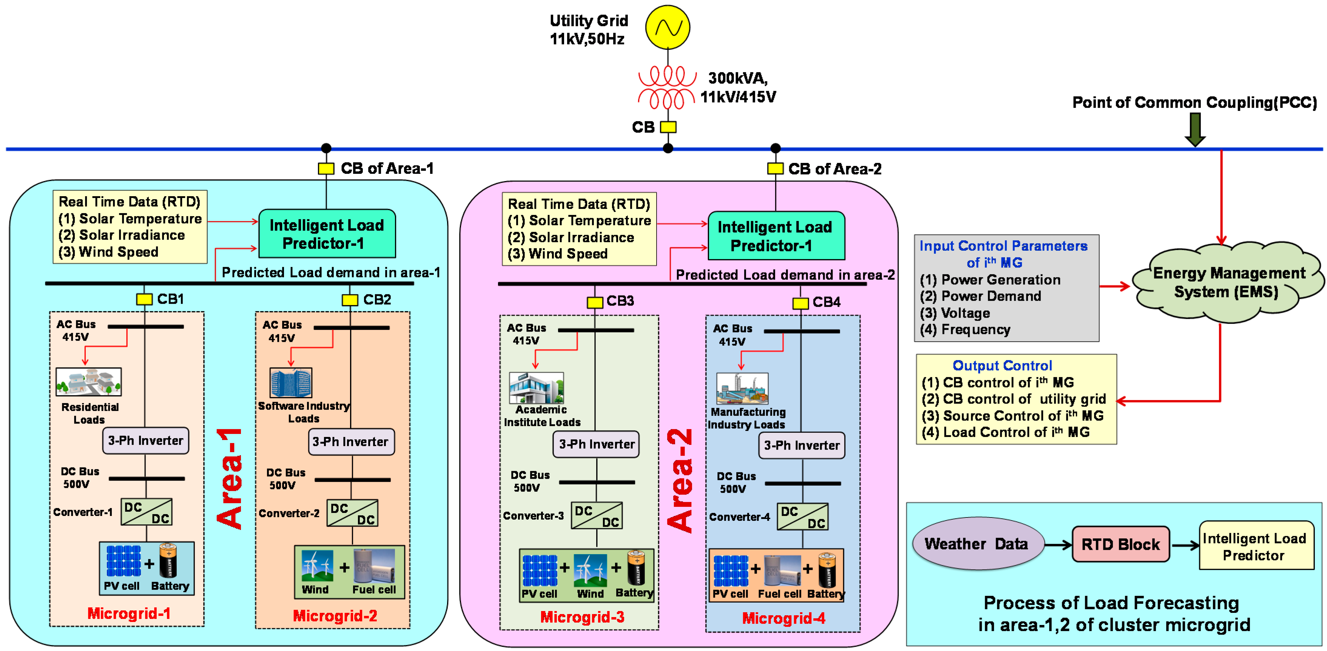
2. Description of the Proposed Cluster Microgrids

The cluster microgrids is also known as the interconnected microgrid system and is formed by interconnecting four neighborhood microgrids, as shown in Figure 1. It shows the layout of the “Cluster Microgrid” system considered for the study.
The proposed system is separated into two areas: area-1 and area-2, both of which are deemed interoperable inside the cluster. Area-1 is formed by connecting Microgrid-1 (Residential Building) and Microgrid-2 (Software Building) and area-2 is formed by connecting Microgrid-3 (Academic Institute Building) and Microgrid-4 (Manufacturing Industry Building) in the selected location. These interconnected and interoperable areas are further integrated into the conventional grid through the Common Coupling Point. Each area in the cluster microgrids is equipped with renewable sources which are available freely in that location and also consists of two microgrids with local agent controllers of that building and an intelligent forecaster with a Real-Time Data (RTD) measurement block. The interrelated cluster microgrid is considered in such a way that it has to operate in both self-standing modes and also in grid-related modes. The RTD block collects the real-time information on solar temperature, irradiance, speed of the wind turbine, and predicted load demand from the selected location. The output data from the RTD block is applied to the corresponding intelligent predictor for forecasting. Forecasted load demand information of the cluster microgrid is applied as an input for the energy management system to function effectively. Correspondingly, the energy management system produces the control signals to the circuit breaker to import or export based upon the energy needs. The energy management system in this architecture is designed to make the energy transactions during excess/deficit power conditions to/from the neighborhood area or utility grid. However, the complete modelling of all renewable sources and constituents is given in [28]. Table 1 contains the information on various parameters considered for the simulation of the cluster microgrid system.

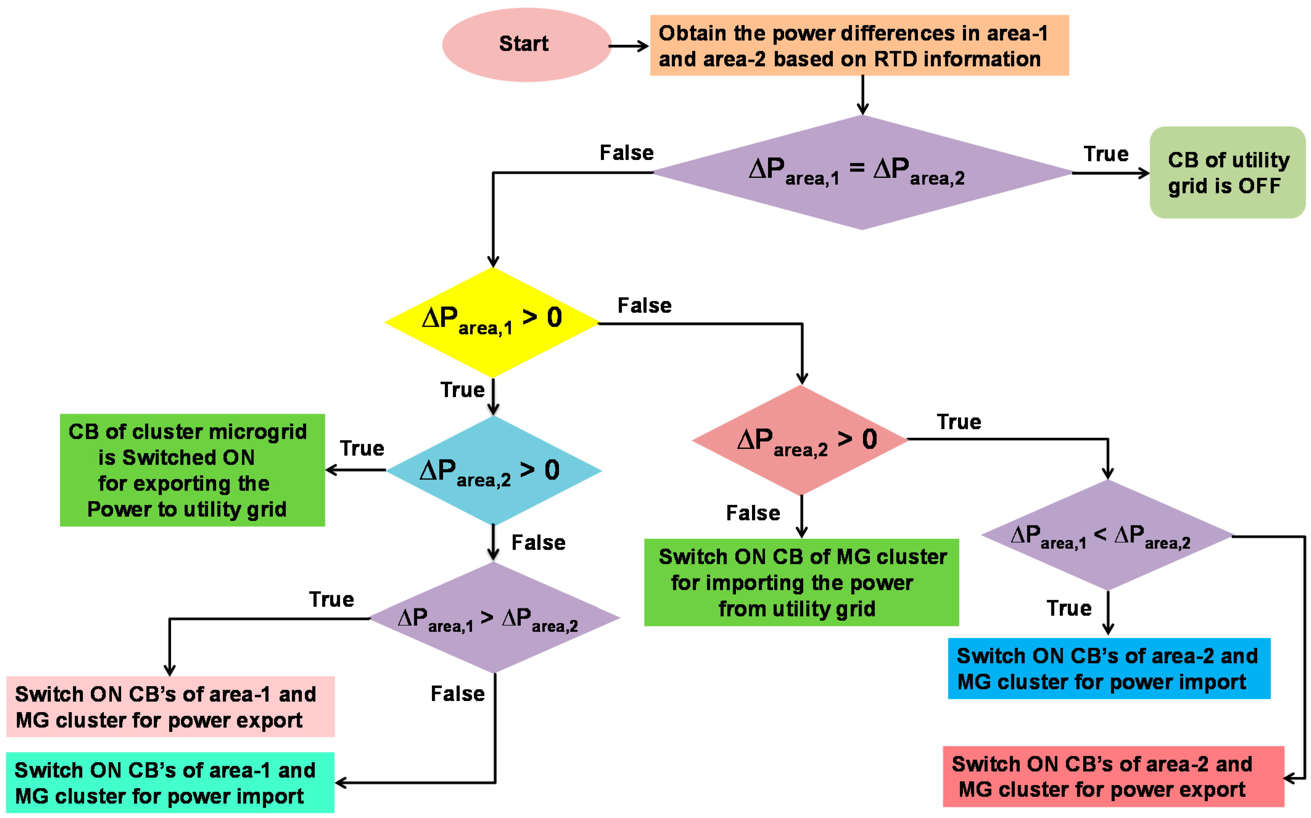
Energy Management System (EMS)

An energy management system (EMS) is an information system on a software platform that supports the functionality of generating, transmitting, and distributing electrical energy at a low cost, according to the international standard IEC 61970. Energy management in microgrids is a computer-based control method that ensures the best functioning of the system. In a variety of ways, a microgrid must optimize the usage of renewable energy sources.
Machine interfaces and supervisory control and data acquisition systems (SCADA) are two EMS components that carry out decision-making procedures [28,29]. This EMS is implemented in the proposed cluster microgrid system to manage the resources connected to all microgrids. This ensures that energy transactions are seamless and that grid frequency is maintained under dynamic load conditions. The flowchart for implementing the EMS is shown in Figure 2.
The economic benefit to the consumer can be enhanced by utilizing on-site distributed generators and lowering reliance on the main grid. The EMS consists of a central controller with direct commands to each distributed energy resource in each microgrid, data acquisition of microgrid operation characteristics and parameters, and information acquisition from the forecasting system, all of which are used to optimize appropriate unit commitment and resource dispatch in relation to the preset objectives. Three layers are incorporated into the cluster microgrid system, namely an external layer that is dedicated to data collection (live weather data, electricity consumption data, etc.), a prediction layer that is used to predict weather conditions and local demand, and an operational layer that consists of energy management algorithms, which are implemented to dynamically regulate energy flow among the devices based on prediction data. The goals of this centralized control algorithm are to forecast energy and electricity load, govern dynamic energy management, and send commands to physical equipment to respond appropriately.

3. Machine Learning Techniques

3.1. Linear Regression (Quadratic)

The model is called linear regression, which optimizes the fit of functions to training data by utilizing the squared Euclidean distance metric. In the simplest model y = λ 1 x + λ 0 , a straight line with gradient λ 1 is fitted to the data, and the intercept of y is λ 0 . The depiction of a linear regression model is given in Equation (1) [30].
To map the relationship between terms x i and x j , interaction terms x i x j might be used. If the effect x i on y is dependent on the other factors x j , j i , this produces better results than a simple linear regression given in Equation (2). In a quadratic model, a quadratic function is fitted to the data and optimized using least squares. As a result, as shown in Equation (3), the model has an intercept, linear terms, interactions, and squared terms. Figure 3 shows the flowchart for implementing the linear regression model in the MATLAB/Simulink environment.
y = λ 0 + λ 1 x 1 + λ 2 x 2 + + λ n x n
y = λ 0 + λ 1 x 1 + λ 2 x 2 + + λ n x n + λ 12 x 1 x 2 + + λ 1 n x 1 x n + + λ ( k 1 ) k x k 1 x k
y = λ 0 + λ 1 x 1 + λ 2 x 2 + + λ n x n + λ 12 x 1 x 2 + + λ 1 n x 1 x n + + λ ( k 1 ) k x k 1 x k + λ 11 x 1 2 + + λ k k x k 2 }

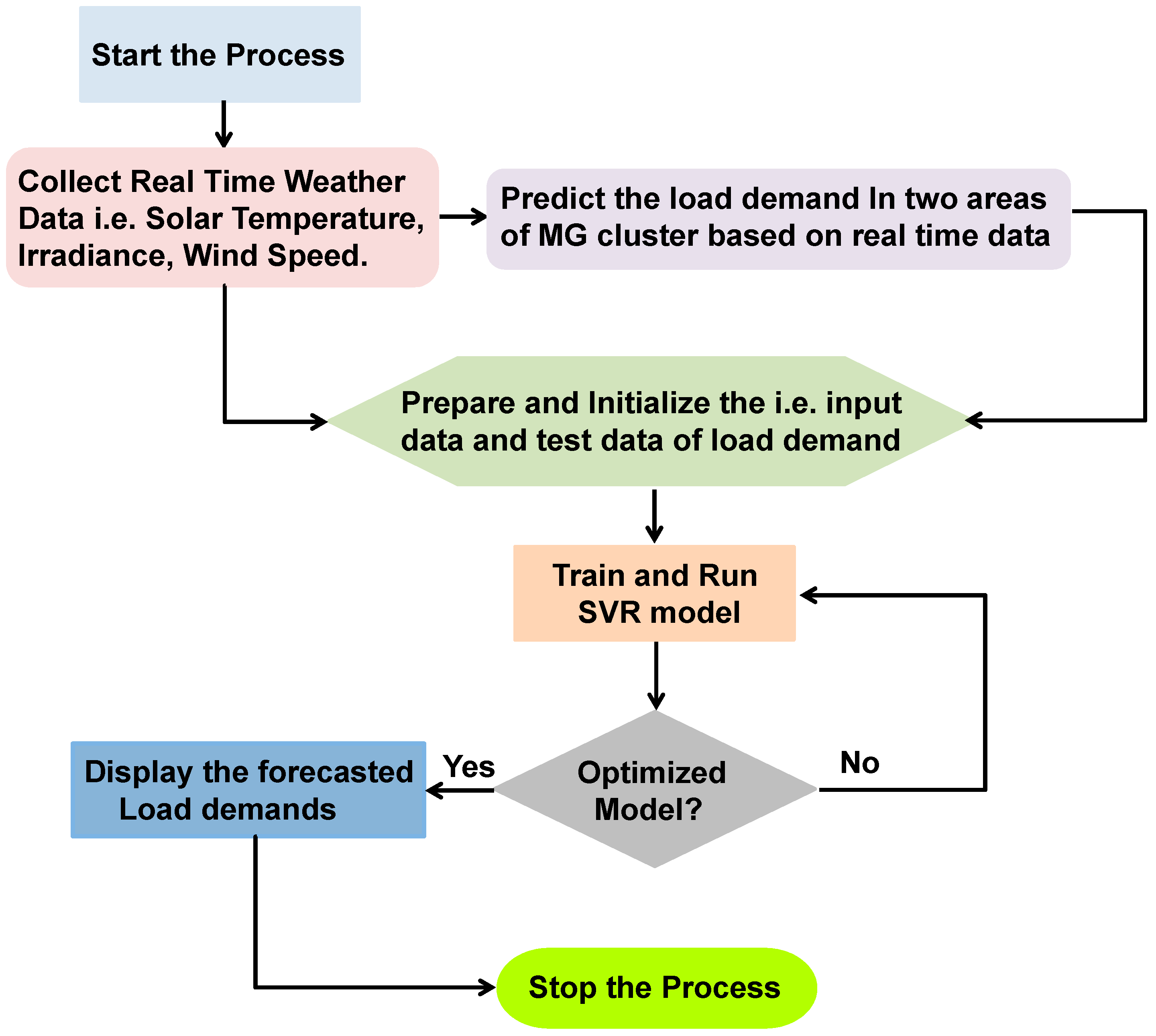
3.2. Support Vector Machine

Machine learning approaches for data classification and regression, such as support vector regression (SVR) and support vector machines (SVMs), have been used to forecast the electric load demand. Vapnik proposed the support vector machines (SVMs) in 1995. The SVR’s main premise is to map the original data “ α ” nonlinearly into a higher dimensional feature space. Hence, the training dataset is given as { ( α n , β n ) } n = 1 k , in which the input vector is α n ; the target vector is β n , and k is the total number of data patterns of the training data. The target of SVM is to generate a decision function of SVM in Equation (4) by minimizing the risk function given in Equation (5) [31].
μ = τ ( α ) = ω · ρ ( α ) + θ
R R = M k i = 1 k L ( β i , τ ( α ) ) + 0.5 ω 2
Therefore, the function value,
L ( β i , τ ( α ) ) = { | β i τ ( α ) | ε ;   i f   | β i τ ( α ) | ε 0   i f   | β i τ ( α ) | < ε .
The following is the terminology used in Equations (4) and (5):
ω —Weight vector used to control the model smoothness;
θ —“Bias” parameter;
ρ ( α ) —High-dimensional space which is mapped nonlinearly into input space α ;
M k i = 1 k L ( β i , τ ( α ) ) —Empirical risk function;
0.5 ω 2 —Regularization term used to determine function complexity;
ε —Tube size (user determined);
M —Regularized constant (user determined).
Two positive slack variables, namely ϕ , ϕ * , are incorporated to signify the distance between original values and the ε -associated tube’s edge values; then, Equation (5) is converted to the form given in Equation (6).
min ( R R ) = M · i = 1 k ( ϕ i + ϕ i * ) + 0.5 ω 2
Subjected to the constraints
β i ω α i θ ε + ϕ i ; i = 1 , 2 , 3 k ω α i + θ β i ε + ϕ i * ; i = 1 , 2 , 3 k ϕ i ϕ i * 0 , i = 1 , 2 , 3 k
Using primal Lagrangian, the dual optimization problem of the above primal one is obtained as follows [31,32].
L ( ω , θ , ϕ i , ϕ i * , μ i , μ i * , Ω i , Ω i * ) = 0.5 ω 2 + M ( i = 1 k ( ϕ i + ϕ i * ) ) i = 1 k Ω i [ ε + ϕ i + ω ρ ( α i ) + θ β i ] i = 1 k Ω i * [ β i + ε + ϕ i * ω ρ ( α i ) θ ] }
The above Equation (7) is minimized by using variables ω , θ , ϕ i , ϕ i * and is maximized with respect to μ i , μ i * , Ω i , Ω i * ; so, the following Equations (8)–(11) will be obtained.
L ω = ω i = 1 k ρ ( α i ) ( ϕ i ϕ i * ) = 0
L θ = i = 1 k ( Ω i Ω i * ) = 0
L ϕ i = M Ω i μ i = 0
L ϕ i * = M Ω i * μ i * = 0
Applying Kuhn–Tucker conditions to regression and Equation (6) gives dual Lagrangian by substituting Equations (8)–(11) into Equation (7). The following Equation (12) is the dual Lagrangian function obtained by considering the kernel function as K ( α i , β i ) = ρ ( α i ) ρ ( α j )
ψ ( Ω i , Ω i * ) = i = 1 k β i ( Ω i Ω i * ) ε i = 1 k ( Ω i + Ω i * ) 0.5 i = 1 k j = 1 k ( Ω i Ω i * ) ( Ω j Ω j * ) K ( α i α j )
Subjected to the constraints
i = 1 k ( Ω i Ω i * ) = 0 ;   where   0 Ω i M ; i = 1 , 2 , 3 k 0 Ω i * M ; i = 1 , 2 , 3 k
The Lagrangian multipliers defined in Equation (12) must satisfy the equality constraint Ω i Ω i * = 0 . Hence, the regression function is obtained as given in Equation (13).
τ ( α , Ω , Ω * ) = i = 1 m ( Ω i Ω i * ) K ( α , α i ) + θ
Figure 4 shows the sequence of steps to be considered for implementing the support vector machine model in the MATLAB/Simulink environment.

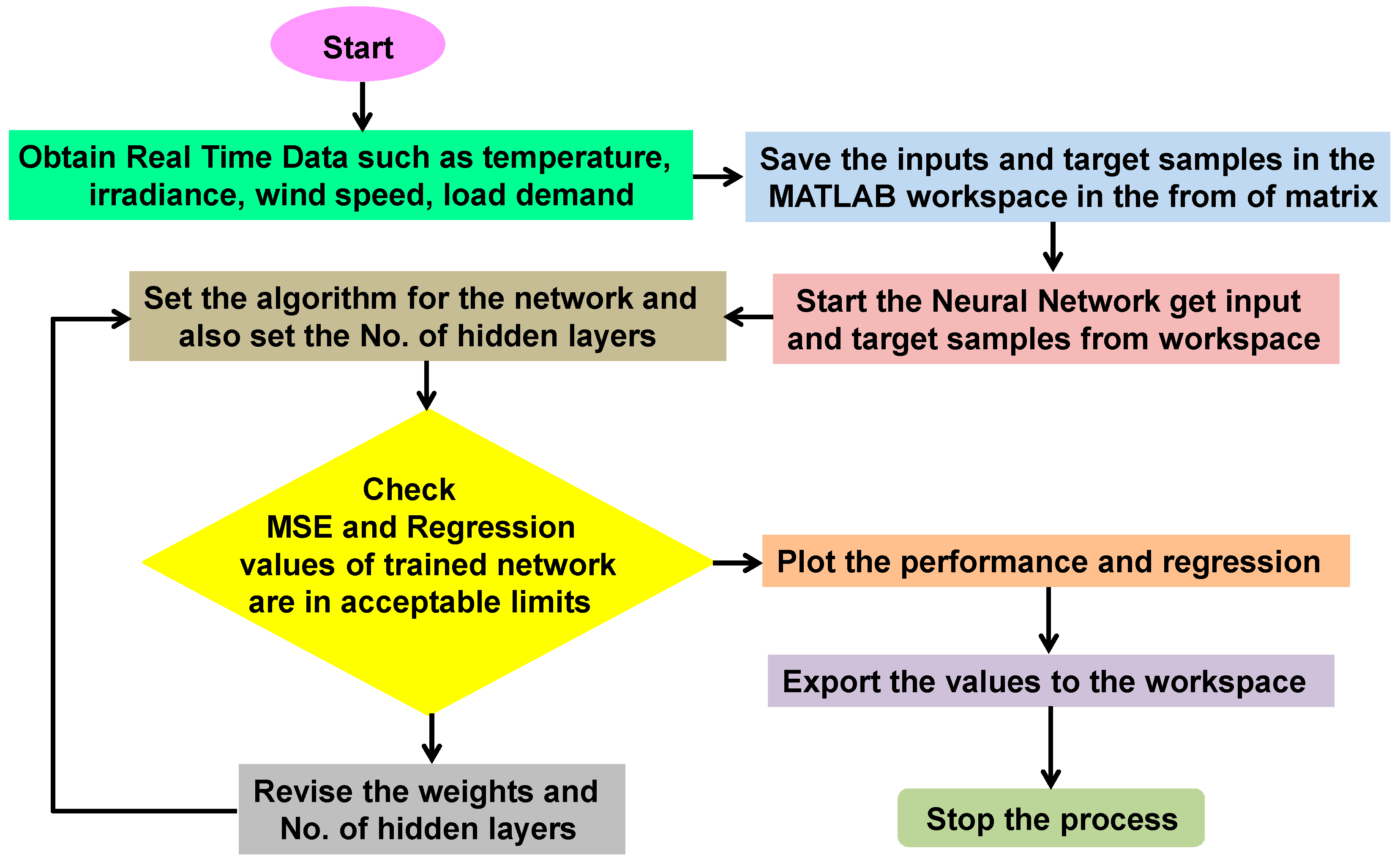
3.3. Artificial Neural Networks (ANN)

In this article, as an application of artificial intelligence (AI), an artificial neural network (ANN) is employed as an intelligent predictor. The concept of ANN was introduced several years ago for different applications because of its capacity to forecast the data and also to control the system response effectively. It has been demonstrated that ANN is one of the effective solutions for all forms of real-time nonlinear issues. An artificial neural network (ANN) is designed based on the interconnection of processing elements that carries information. McCulloch et al. first introduced various neural network architectures, such as single layer and multilayer feed-forward networks, which are explained as follows [33].

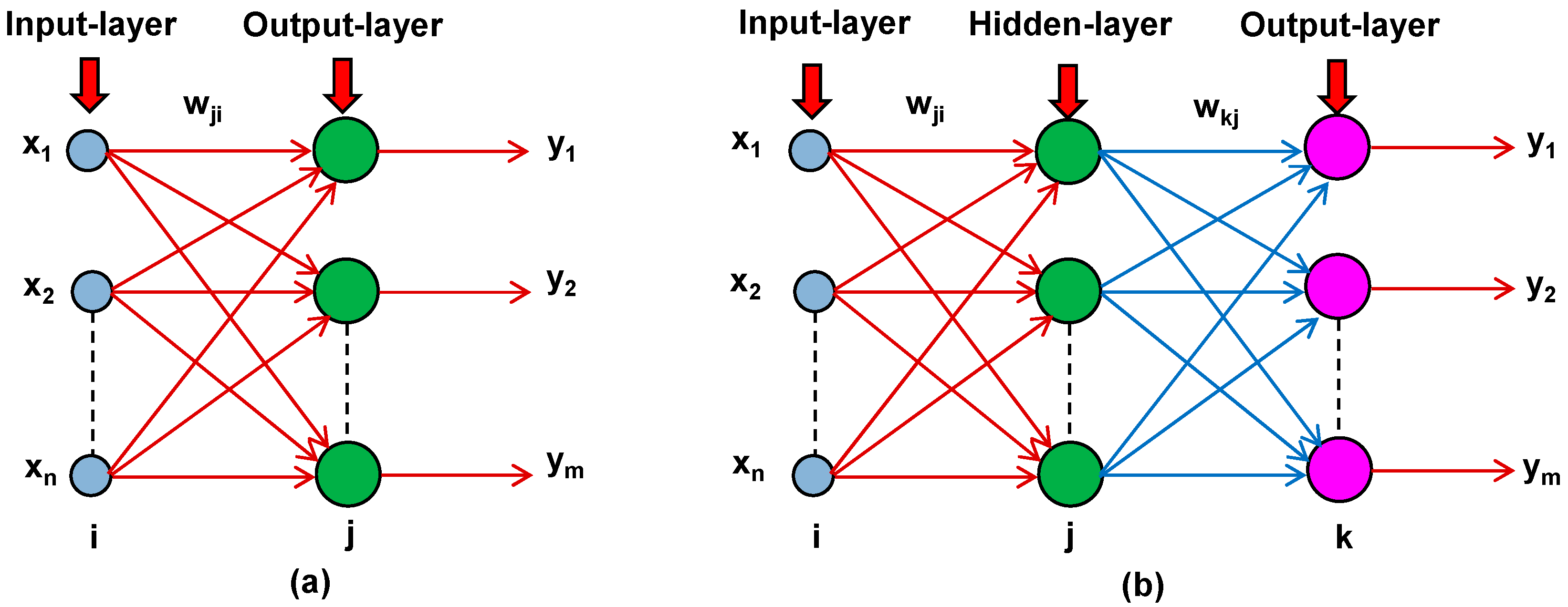
3.3.1. Single Layer Feed Forward Network

In this schematic view, the network has two layers, namely the input and output layers. The primary function of the input layer is to transmit signals to other neurons. The neurons in the input layer receive the input signals in the input layer, and the output layer neurons send output signals. In this type of structure, the signals are transferred from the input layer to the output layer but vice versa is not possible, so it is named a feed-forward network. The general architecture is as shown in Figure 5a, where x 1 , x 2 , x 3 x n are the input layer elements and y 1 , y 2 , y 3 y m are the output layer elements, and w j i are the weights associated between the input and output layer.

3.3.2. Multi-Layer Feed Forward Network

This network consists of one input layer, one output layer, and single or multi hidden layers. The processing elements for the hidden layer are hidden neurons only. Before sending the inputs to the output layer, computation is performed by hidden neurons in the hidden layer. The general schematic is shown in Figure 5b. Here, w j i is the weight that links input and hidden layers and w k j is the weight that links hidden and output layers.
Figure 6 depicts the flowchart of the intelligent predictor, i.e., artificial neural network (ANN), which is to be implemented in the Simulink environment. ANN is very flexible and can be easily adaptable to all complex nonlinear problems. The following are the steps to be taken for training the ANN with different weight updating algorithms:
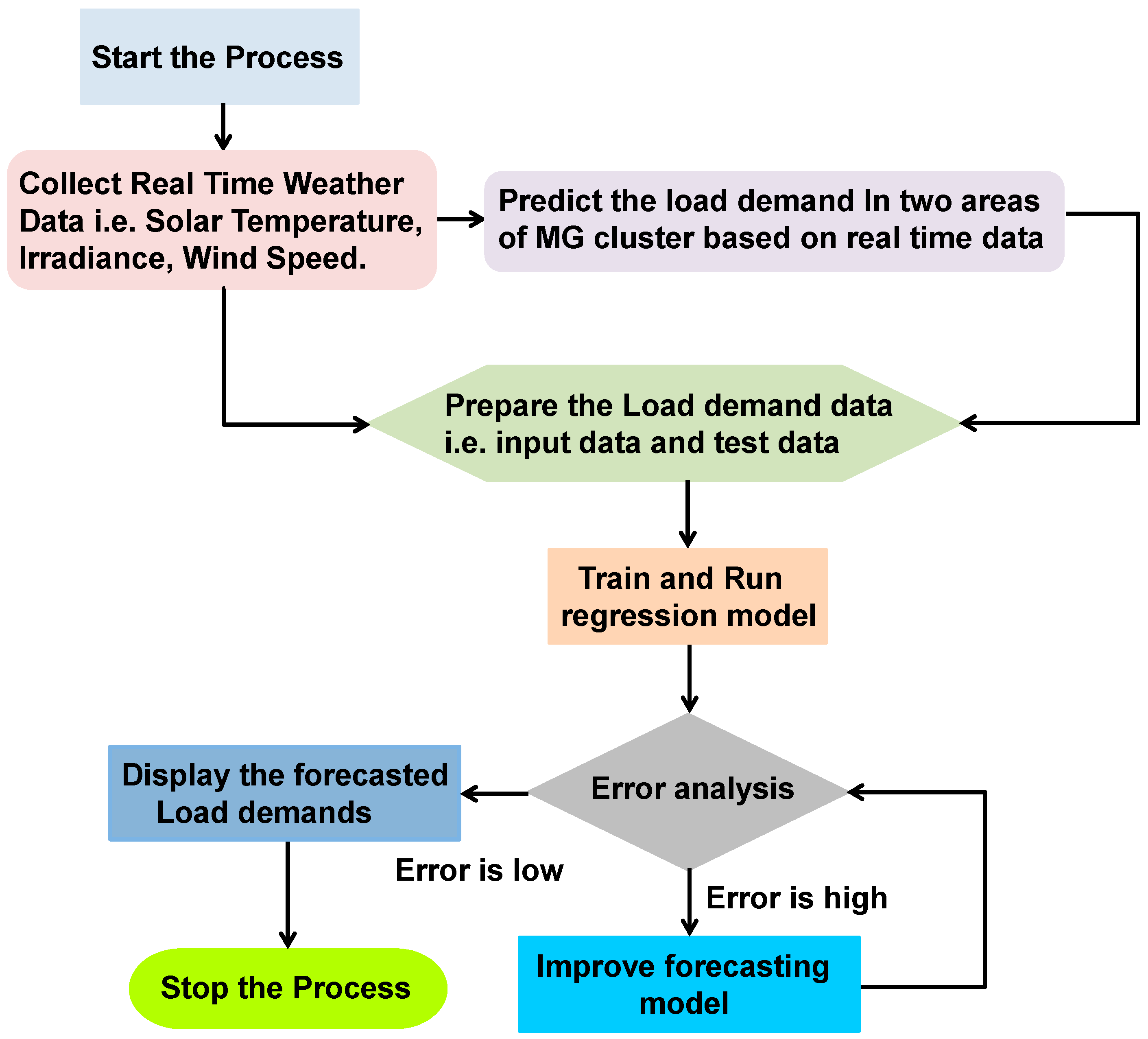
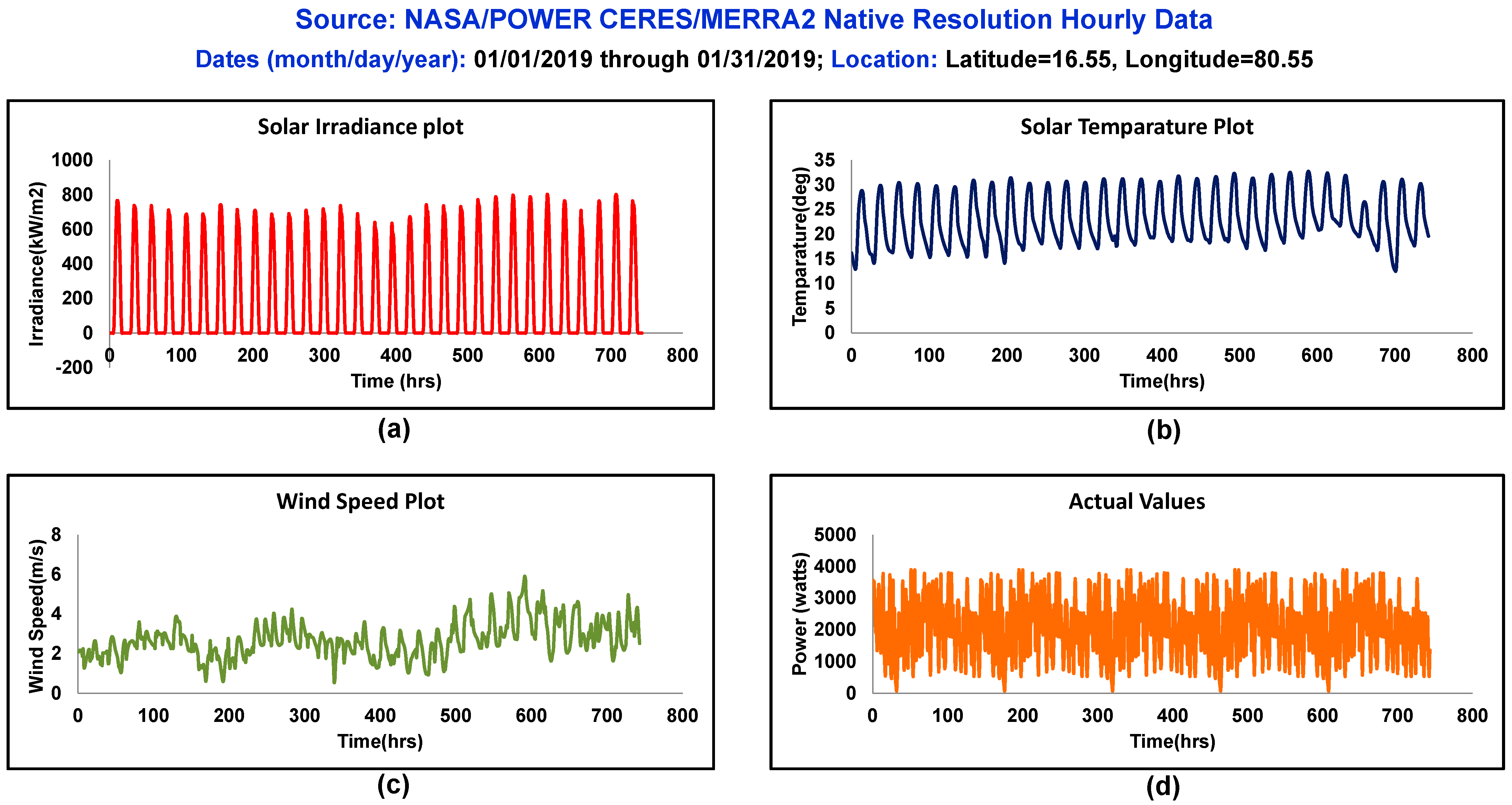
  • Select the input data, such as temperature, Diffuse Horizontal Irradiance (DHI), wind, and loads from selected locations;
  • Select the number of hidden layers;
  • Select proper active function for hidden and output layers.
For all feed-forward (FF) networks, the relationship between inputs, hidden, and output samples are obtained from Equations (14) and (15).
ψ k = ζ n ( j = 0 h ω ( n ) θ j . ρ j )
where , ρ j = ζ n 1 ( i = 0 N ω ( n 1 ) j i μ i )
Here, N is the input layer dimension, h - is a hidden layer dimension, k is the output layer dimension, ω ( n ) θ j is the output layer weight, ω ( n 1 ) j i is the hidden layer weight, and ζ n is the activation function used for the feed-forward neural network.

4. Results’ Validation and Discussion

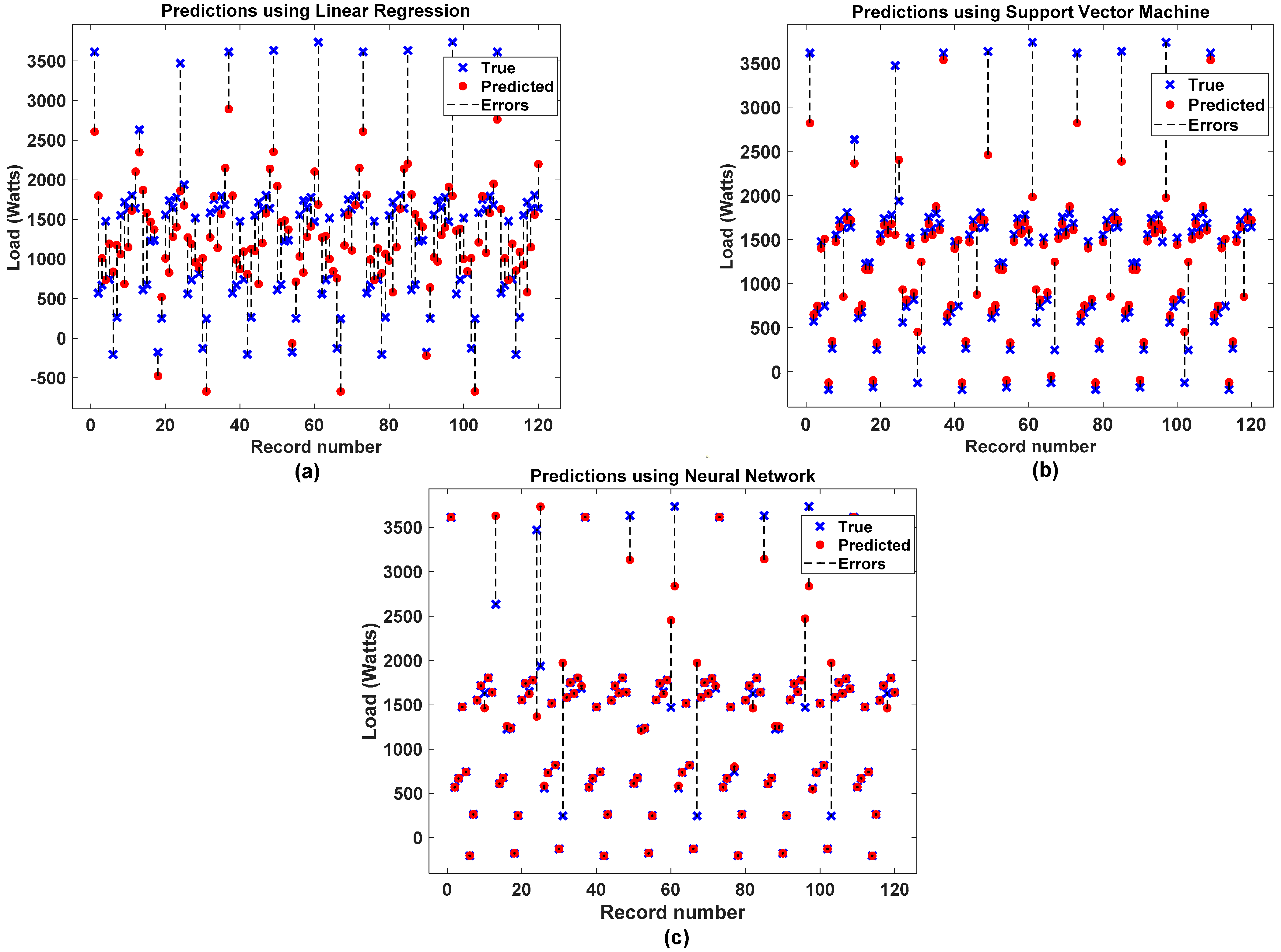
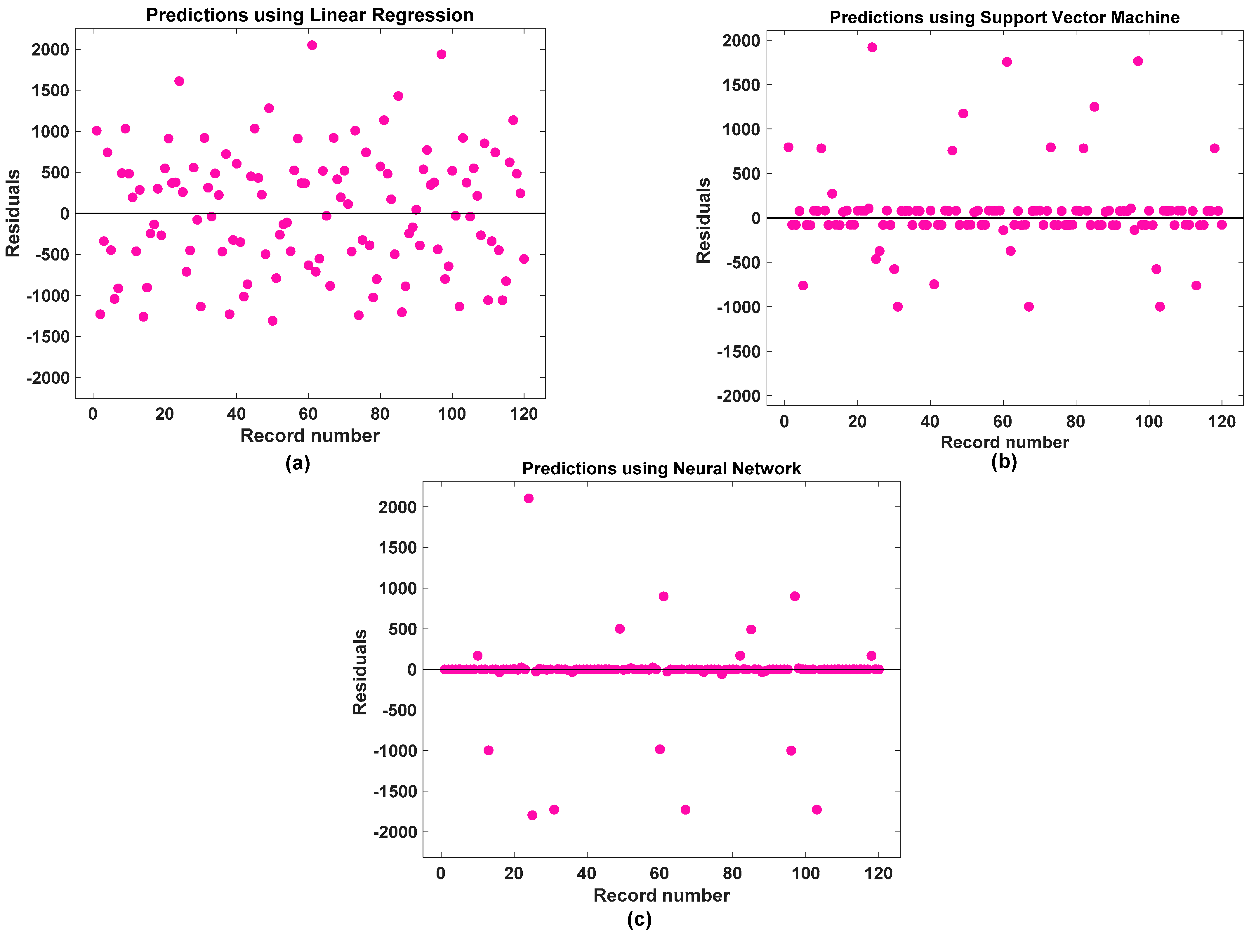
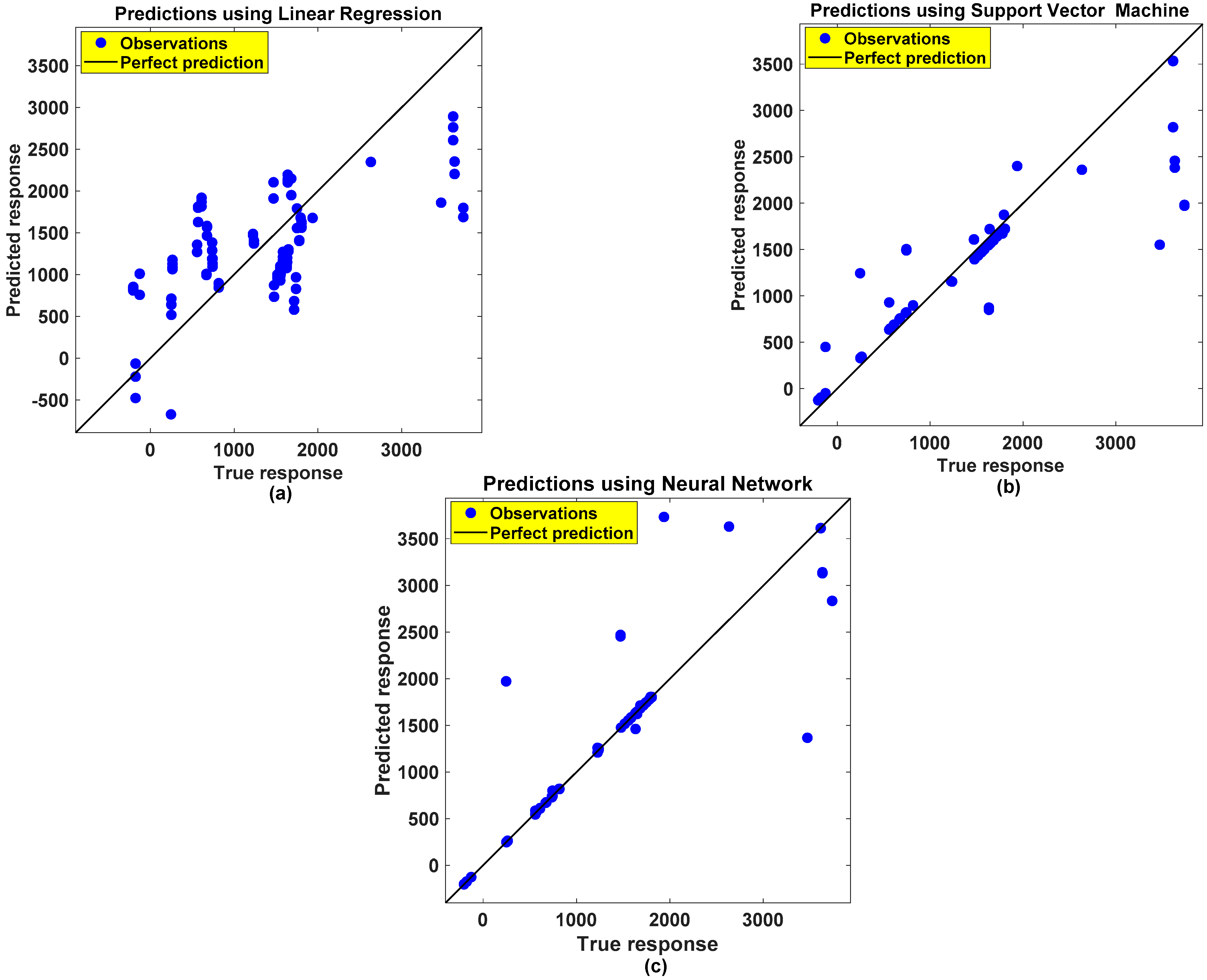
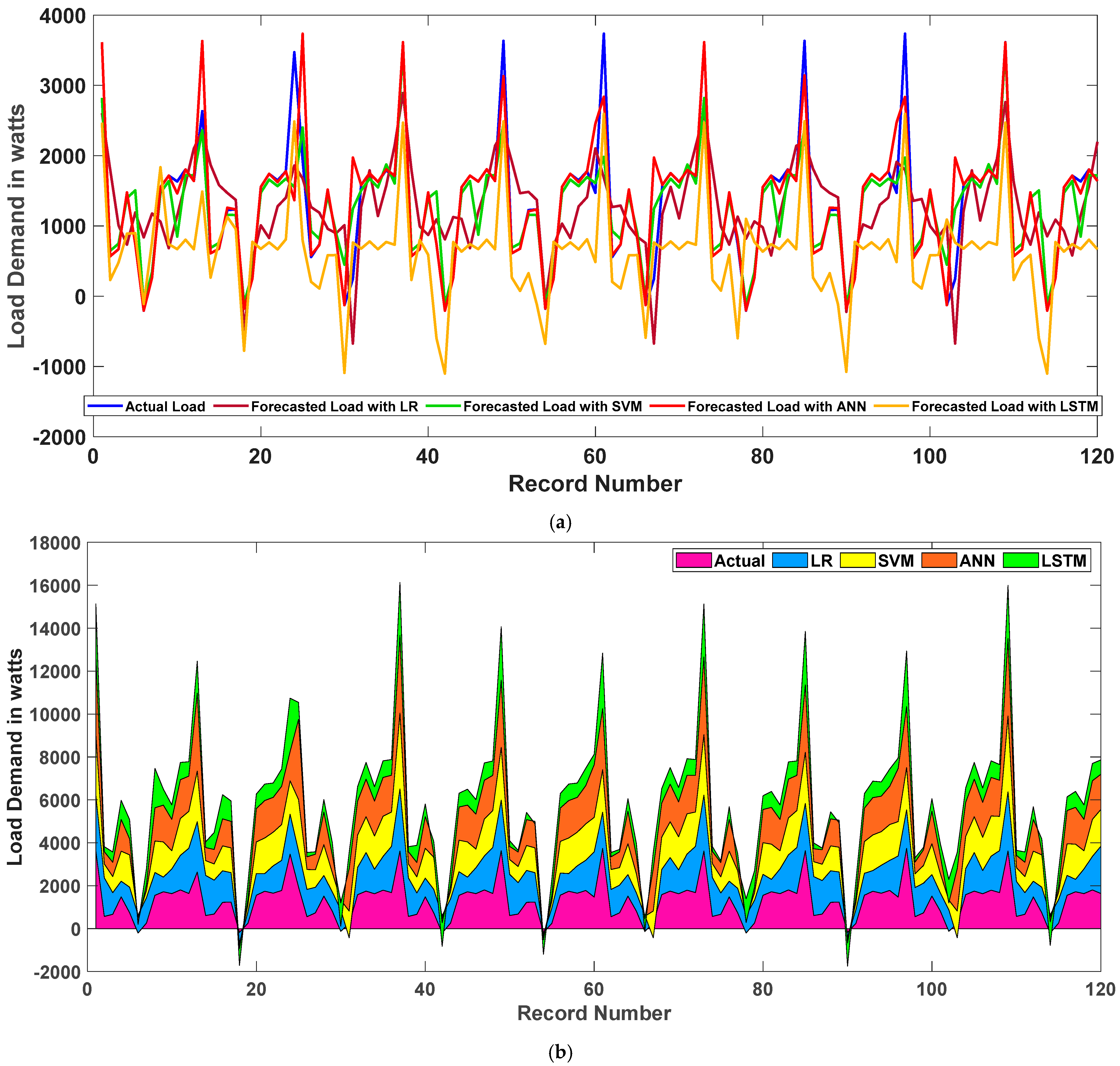
4.1. Day-Ahead Load Demand Forecasting Using Linear Regression, Support Vector Machine, and Artificial Neural Networks

The goal of this work is to determine the best day-ahead load demand forecasting solution in cluster microgrids. We gathered data on solar and wind factors from Vijayawada city in the state of A.P., India, with a “location ID” of 44665, a latitude of −16.65°, and a longitude of −80.65° [34,35]. Figure 7a–d shows the characteristics of the actual dataset, such as solar irradiance, temperature, wind speed, and the electric load consumption in a specified location for one month from 1 January 2019 to 31 January 2019. Test data are considered for the period from 10 January 2019 to 16 January 2019. Our job is to calculate daily, weekly, and monthly electricity usage by predicting consumption for each hour of the day. Machine learning algorithms anticipate the future value of a time series data collection by discovering correlations between historical data attributes and using the revealed associations to forecast the future value.
Pre-processing is essential for improving data quality and the effectiveness of machine learning algorithms. In each machine learning (ML) model, normalization and data transformation are two common pre-processing procedures. The variables in a cluster microgrid dataset are spread across various ranges, resulting in a bias favoring values with greater weights, lowering the effectiveness of the framework. A zero-mean normalization technique is employed in the study for data normalization on the load and temperature variables because attribute normalization improves the convergence rate and numerical stability of NN training.
Data must be quantifiable because machines process them using mathematical calculations. Data encryption is performed during data pre-processing, which converts quasi inputs to numeric inputs before giving them to ML frameworks because the majority of the dataset contains both category and numerical information. The data are then separated into training and testing datasets. The training dataset is used to create the machine learning algorithms, which are then tested against a new dataset to see how well they perform. In this study, 30% of the dataset is used to evaluate the performance of the developed ML algorithms, whereas 70% is used to comprehend the ML algorithms [25]. The “MATLAB/Simulink software 2021a” is used to model the proposed cluster microgrid and also to execute the machine learning algorithms.
In this work, we have obtained the real-time information of solar temperature, irradiance, and wind speed in the two interoperable areas at the abovementioned location and then obtained the loads in area1 and 2 concerning the real-time values, which are then applied as four inputs to the intelligent predictor to forecast the load demand in the next 30 days; then, the total estimated forecasted power at the PCC of the cluster microgrid is given to the EMS of the system. The EMS then generates control signals to export/import power to/from the central utility grid.
The stress on the electrical grid is lowered as a result of providing consumers with more reliable and efficient power. Figure 8 shows the performance plots of various machine learning algorithms used in this work for day-ahead load demand forecasting for the aforesaid period considered for the study. The plot is drawn by taking 120 data samples on the x-axis and the predicted load on the y-axis.
The actual and predicted values are shown in the plot and also error values are marked with dashed lines. From the plot, it is observed that the performance of the neural network regression model gives more accurate load demand forecasted values when making the comparison with the remaining LR (quadratic) and SVM models. A residual measures how far a point is vertically from the regression line. To visually confirm the correctness of the machine learning model, we must use residual plots. Plotting all residual values across all independent variables can be tricky, so we can either make separate plots or use other validation statistics, such as adjusted R2 or MAPE scores.
So, Figure 9 shows the typical residual plots of all the machine learning methods used. Curve fitting is described as the model that provides the greatest fit to the specific curves in one’s dataset in regression analysis. Linear connections are easier to fit and interpret than curved variable relationships. We use root mean square error (RMSE), R-squared, mean square error (MSE), mean absolute error (MAE), mean absolute percentage error (MAPE), and time of computation metrics to assess the prediction accuracy of each machine learning model in all cases. The forecasting error metrics are obtained as given in Equations (16)–(20).
R M S E = τ = 1 m ( λ τ λ ^ τ ) 2 m
M S E = 1 m τ = 1 m ( λ τ λ ^ τ ) 2
M A E = 1 m τ = 1 m | λ τ λ ^ τ |
M A P E = 1 m τ = 1 m | λ τ λ ^ τ | λ τ
R 2 = 1 ( λ τ λ ^ τ ) 2 ( λ τ λ ¯ τ ) 2
where m is the number of data points, λ τ are the actual values, λ ^ τ are the forecasted values, and λ ¯ τ are the mean values.
Figure 10 shows how the data are fitted for perfect load forecasting using machine learning algorithms. In this, we observed how well the ANN is trained to give the best accurate results. Table 2 gives the comparison of different metrics obtained during the day-ahead load demand forecasting with the use of machine learning algorithms, such as linear regression [30], support vector machine [25,31,32], and artificial neural networks. Later, these results are compared and verified with the time series long short term memory (LSTM) forecasting method [36]. Design parameters of the LSTM method are given in Appendix A. The results show that the artificial neural network regression model effectively forecasts day-ahead load demands in cluster microgrids. So, we propose the ANN is the best machine learning technique for forecasting the day-ahead load demands in cluster microgrids. The performance of various machine learning algorithms considered for the study can be viewed Figure 8, Figure 9 and Figure 10 by considering performance metrics. However, the forecasted values are shown in Figure 11a, which are obtained with respect to the actual values. Similarly, the area plot is given in Figure 11b.

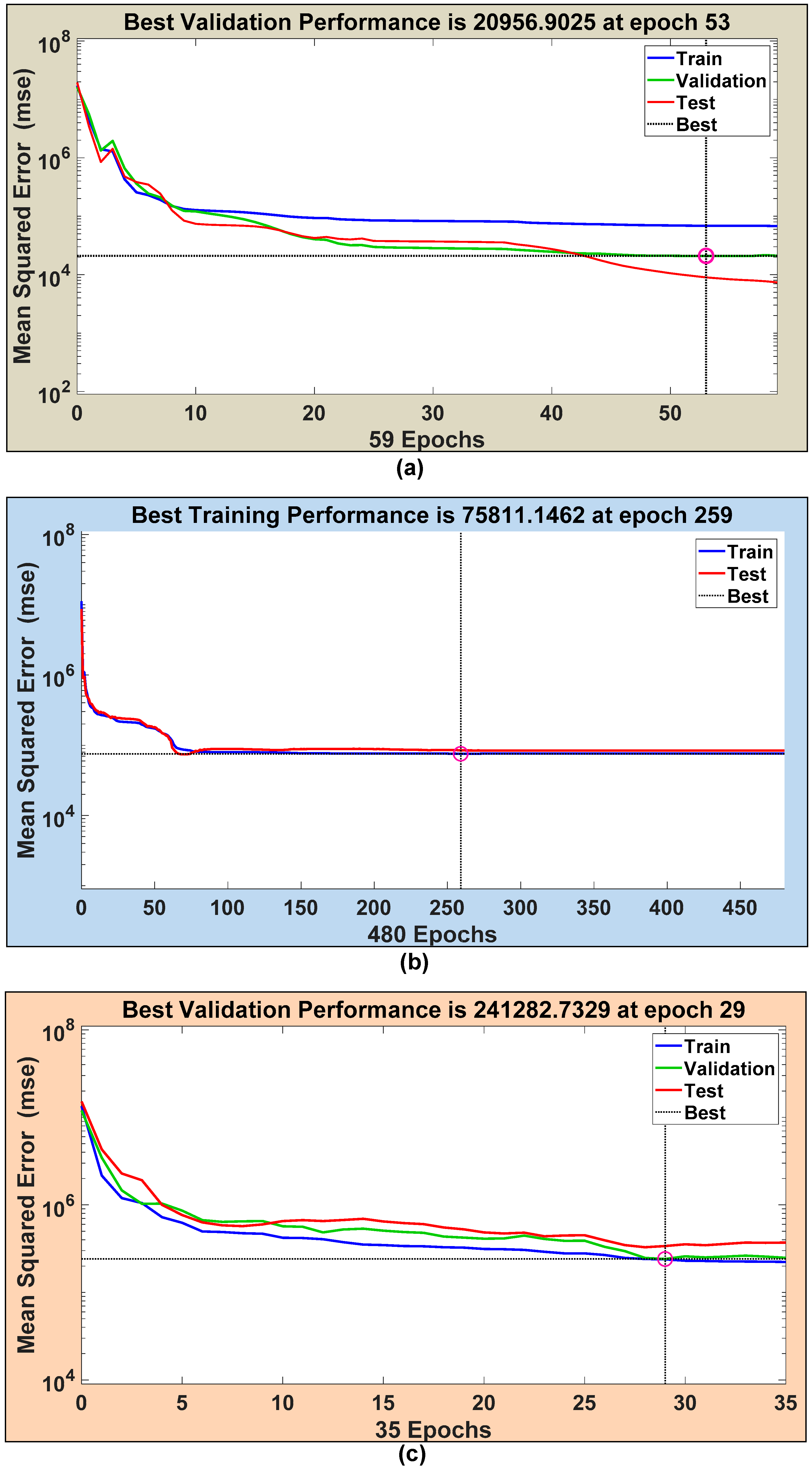
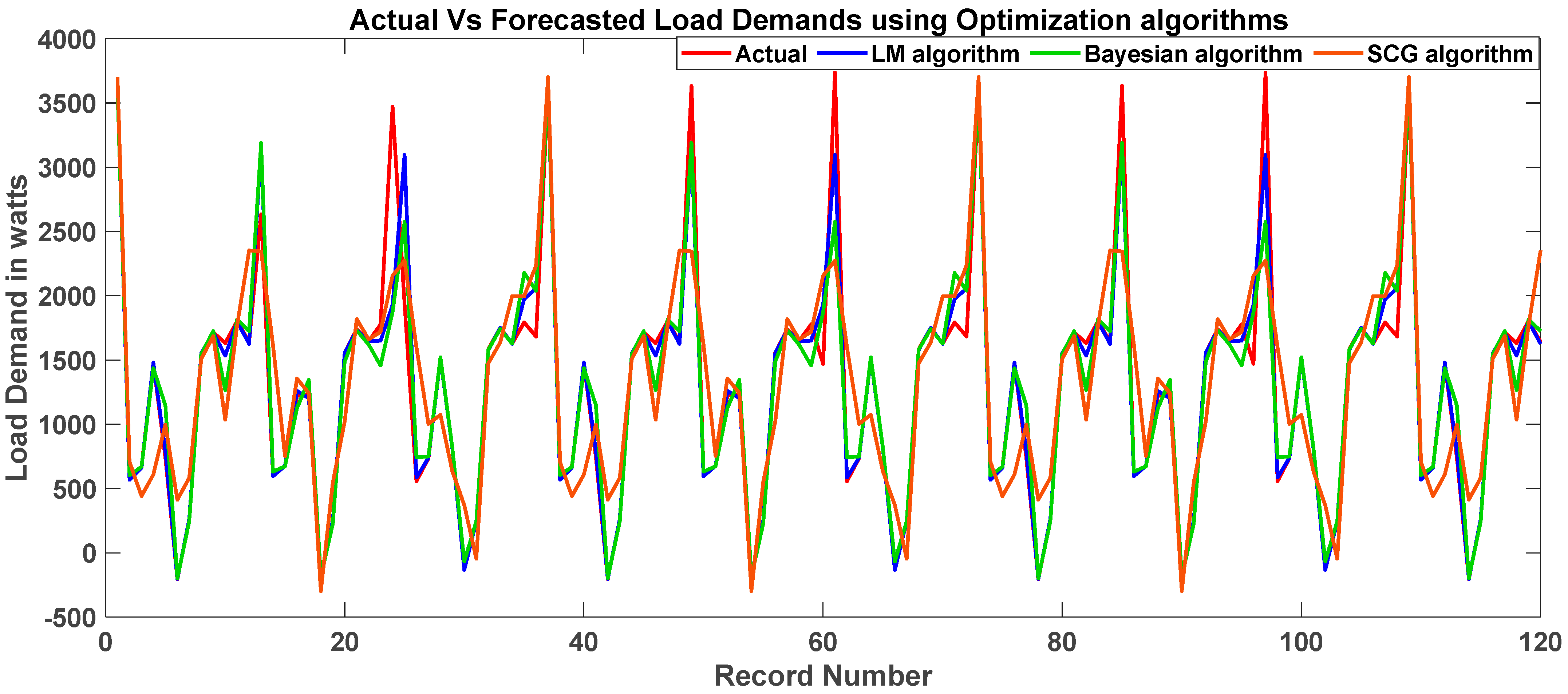
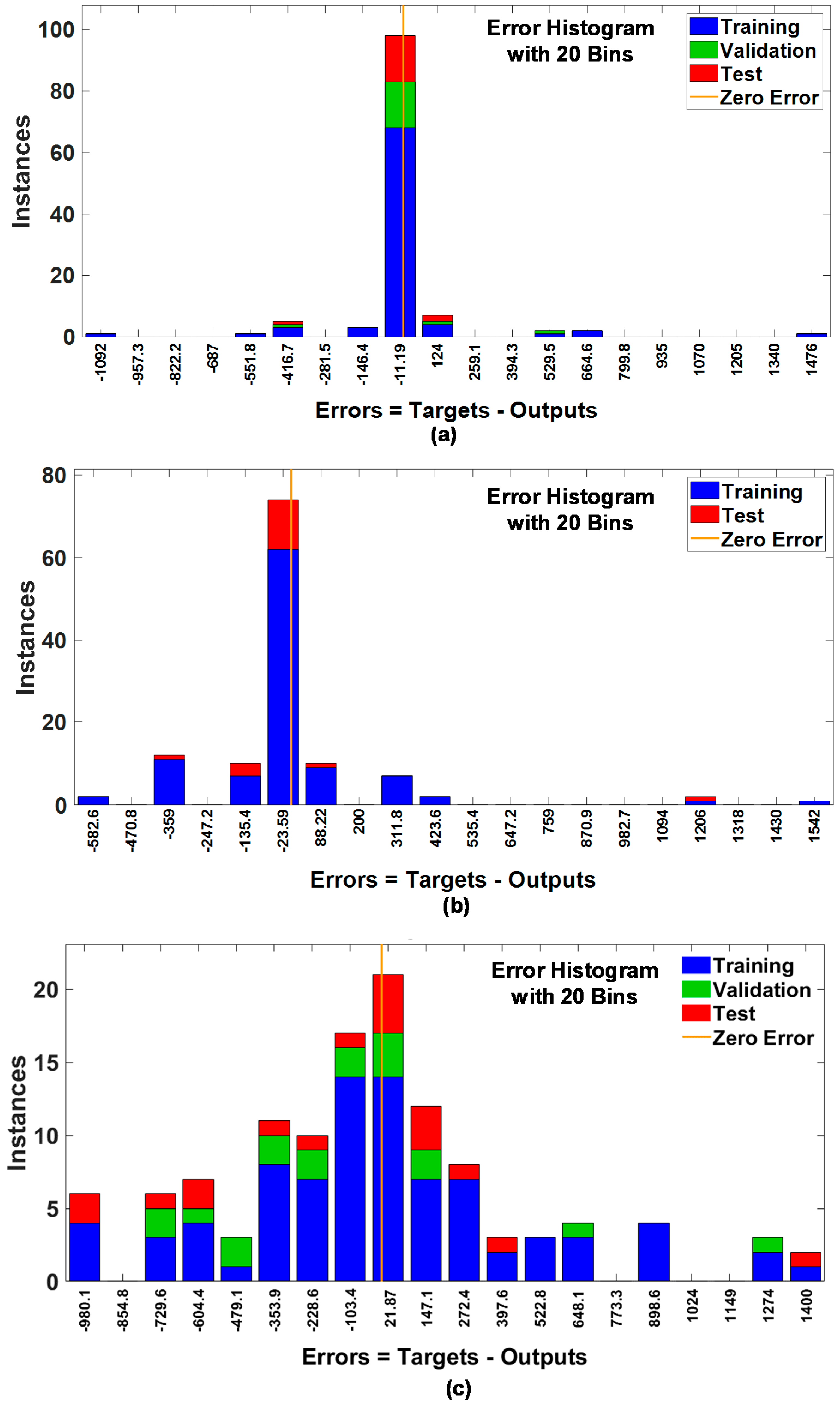
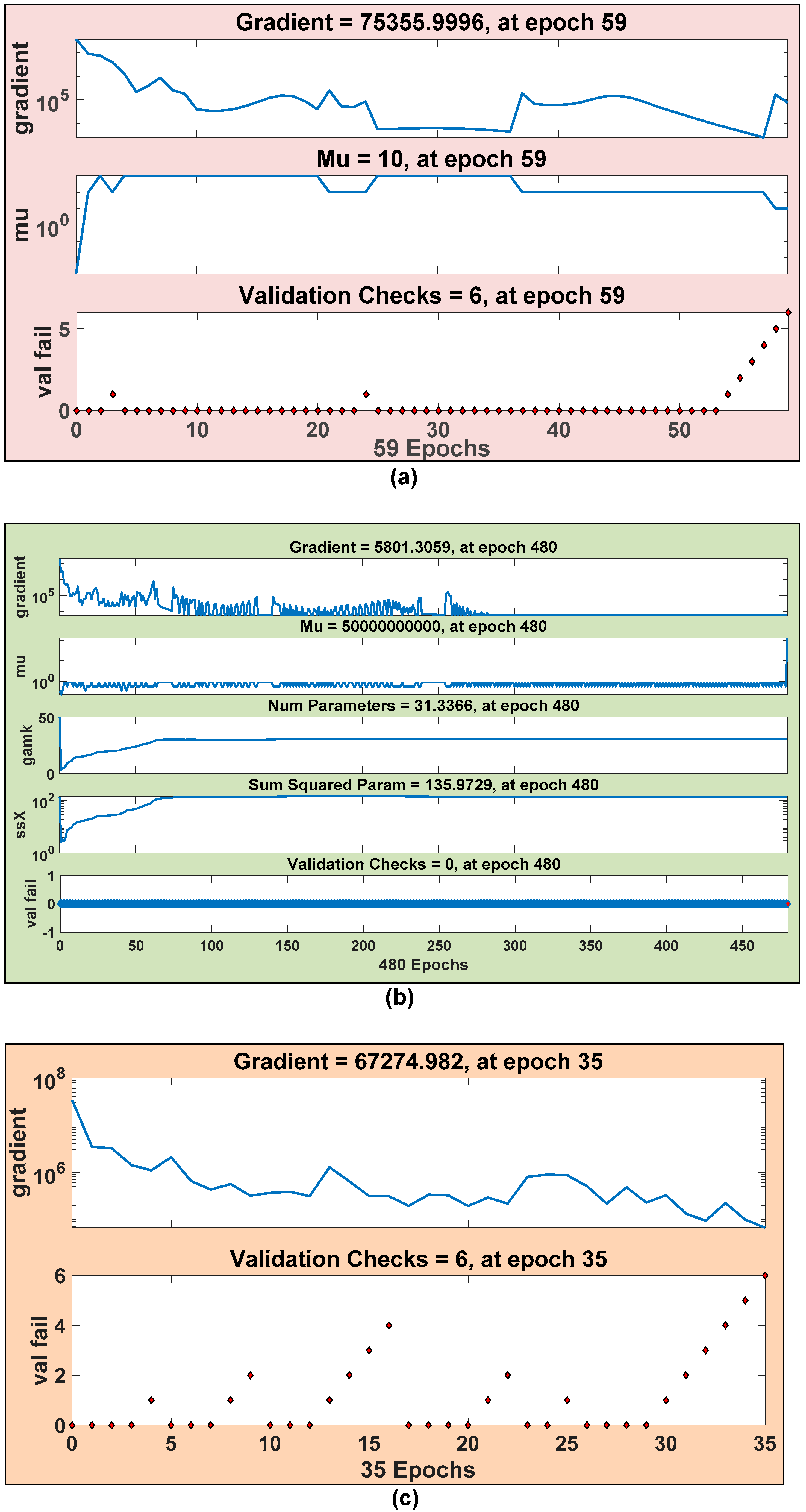
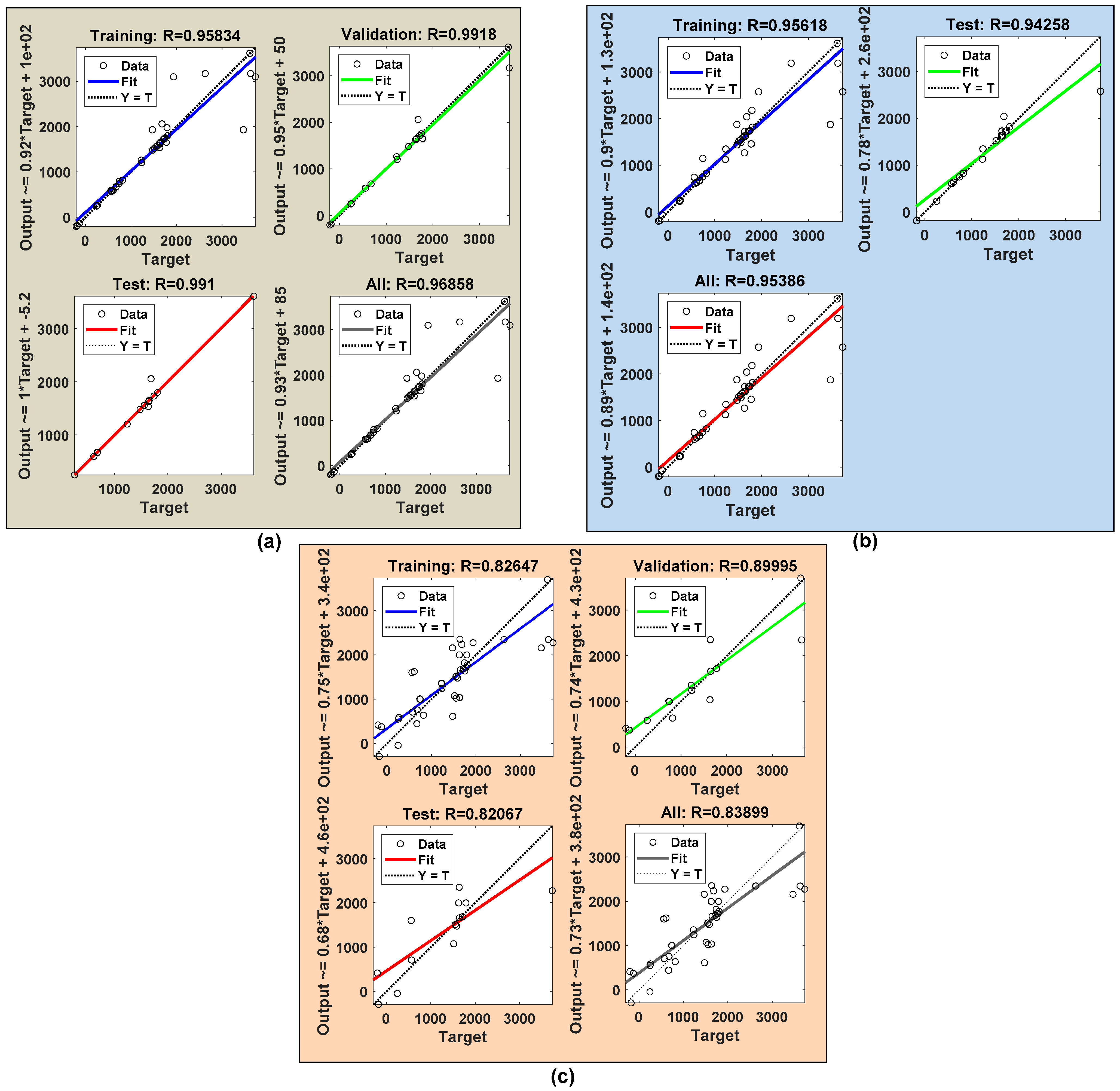
4.2. Identification of Best Optimization Algorithm of Neural Networks for Effective Forecasting

The discussion in the previous Section 4.1 shows that the artificial neural network gives fruitful results in day-ahead load demand forecasting. Hence, in this section, we identified the best optimization algorithm to propose for neural networks for effective functioning. The three optimization algorithms, viz. (1) Levenberg–Marquardt (LM) algorithm, (2) Bayesian Regulation (BR) algorithm, and (3) Scaled Conjugate Gradient algorithm are considered for training the neural networks.

4.2.1. Levenberg–Marquardt (LM) Algorithm

The alternative name for the Levenberg–Marquardt (LM) algorithm is the “Damped Least Square” method. It is particularly designed to work based on the loss function, which is expressed as the sum of squared errors. The approximated hessian matrix is obtained by using the Jacobean matrix and gradient vectors, which are obtained using the following Equations (21) and (22). Jacobean matrix is obtained with the loss function and is given by [33].
J m n = E m W n
where m = 1, 2, 3, …, i; n = 1, 2, 3, …, j; the number of instances in the dataset is “i” and the number of parameters in the network is “j”. The gradient vector is obtained as follows,
H f 2 J T · J + λ I
The further approximated Hessian matrix is obtained from Equation (23),
W ( r + 1 ) = W ( r ) ( J ( r ) T · J ( r ) + λ ( r ) · I ) 1 · ( 2 · J ( r ) T · E ( r ) ) ; r = 0 , 1 , 2 , 3

4.2.2. Bayesian Regulation (BR) Algorithm

The Bayesian Regulation (BR) technique is more efficient than typical backpropagation methods and is based on Bayes’ theorem. The nonlinear regression relations are translated to second-order linear regression-based mathematical equations during the BR process. The most difficult part is deciding on absolute fitting values for the function parameters. The BR framework in ANN works by interpreting provided network parameters probabilistically, which differs from typical training approaches. This chooses a set of weights based on the error function minimization. However, in the BR method, a performance function given in Equation (24) is utilized to find the error, or the difference between real and anticipated data, throughout the training phase. Regularization adds an extra term and function to a BR method to achieve smooth mapping, which uses a gradient-based optimization to minimize the objective and performance function as provided in Equation (25). To address the additional noise present in the targets, the posterior distribution of weights of the neural network will be modified as needed after the data are taken for training [33].
f n = μ t ( τ | ω , a ) + 1 n x = 1 p ( α x β x ) 2
f n = Ω · μ t ( τ | ω , a ) + Ψ μ m ( ω / a )
Here, f n is performance function, μ t is network error values (sum of squares), τ is training set of input and output targets, a is an architecture of neural network which consists of information about the number of layers and their units, μ m is network weights (sum of squares), Ψ μ m ( ω / a ) is weight decay, and Ψ is a rate of decay.

4.2.3. Scaled Conjugate Gradient (SCG) Algorithm

M. Hestenes and Eduard S. created scaled conjugate techniques. These are primarily used to solve linear equations. In conjugate gradient methods, there are numerous sub methods. One of these sub methods is the SCG algorithm. Constrained optimization, curve fitting, and more uses of the SCG algorithm can be found. It uses feed-forward artificial neural networks. These approaches solve when all errors are inside the range of anticipated values. The calculation of the direction of the weights, which is practically difficult, is the most important component of the conjugate methods. Equations (26) and (27), respectively, are the training data and the parameter vector functions. The main drawback of the SCG technique is that it does not supply any data for calculating and inverting the Hessian matrix [33].
S r + 1 = G r + 1 + S r · α x
W r + 1 = W r + 1 + S r · β x ; r = 1 , 2 , 3
where α is SCG parameter, β is the training rate, S o is initial direction vector, and W o is the initial parameter vector. The performance in terms of best validation of the ANN connected in cluster microgrid is attained at epoch 53 with the LM algorithm, at epoch 259 with the BR algorithm, and at epoch 29 with the SCG algorithm, as shown in Figure 12. After training a feed-forward neural network, the error histogram is a histogram of errors between target and predicted values. These error figures can be negative because they represent how expected values depart from target values. The number of vertical bars that appear on the graph is referred to as bins. Here, the entire error range is broken down into 20 smaller bins. The number of samples from your dataset that fall into each category is shown on the Y-axis. The error histogram and also the training states of all optimization algorithms used to train ANN are shown in Figure 13 and Figure 14.
In terms of data training, validation, and testing the values generated by regression demonstrates the relationship between target samples and output samples. If R = 1 on the regression Figure 15, the line is angled at 45 degrees to the x-axis, suggesting that the target and output are the same. When the output sample and the target values are closely related, the value of “R” may be one. If the ANN regression values for all examples are greater than 0.95, the curve fitting is considered to be reasonably valid. From Table 3, it is observed that in all the cases of regression analysis, Levenberg–Marquardt optimization algorithm plays a dominant role. Hence, we proposed LM-based ANN for forecasting day-ahead load demands in cluster microgrids. Actual and forecasted values of day-ahead load demand in the cluster microgrid with different optimization algorithms based on ANN are shown in Figure 16. From the results, it is observed that ANN with the Levenberg–Marquardt optimization algorithm gives fruitful results; hence, we proposed LM algorithm-based ANN for day-ahead load demand forecasting.
In terms of data training, validation, and testing, the values generated by regression demonstrate the relationship between target samples and output samples. If R = 1 on the regression in Figure 15, the line is angled at 45 degrees to the x-axis, suggesting that the target and output are the same. When the output sample and the target values are closely related, the value of “R” may be one. If the ANN regression values for all examples are greater than 0.95, the curve fitting is considered to be reasonably valid. From Table 3, it is observed that in all the cases of regression analysis, the Levenberg–Marquardt optimization algorithm plays a dominant role. Hence, we proposed LM-based ANN for forecasting day-ahead load demands in cluster microgrids. Actual and forecasted values of day-ahead load demand in the cluster microgrid with different optimization algorithms based on ANN are shown in Figure 16. From the results, it is observed that ANN with the Levenberg–Marquardt optimization algorithm gives fruitful results. Hence, we proposed LM algorithm-based ANN for day-ahead load demand forecasting.

5. Conclusions

With the rise of the smart grid, load forecasting is becoming more crucial. As a result, predicting the electrical load with high precision is a difficult assignment. The non-linearity and volatility of real-time energy consumption make it challenging to forecast load demand and consumption. To address this issue, multiple machine learning approaches, such as linear regression (LR), support vector machine (SVM), Long Short-Term Memory (LSTM), and artificial neural networks (ANN) are implemented in this article to estimate electric load demand forecasting in the cluster microgrid context. This work discovered the best models to perform day-ahead load demands by reviewing the validation results for the provided models. This encompasses both the accuracy of their forecasts and the low computational effort required to fit the models and make the predictions. The following are the salient outcomes of the proposed work in this article:
All machine learning algorithms are compared in terms of performance by computing several factors, such as root mean square error (RMSE), mean square error (MSE), mean absolute error (MAE), and calculation time.
Based on the findings, it was identified that artificial neural networks are the best forecasting technique for day-ahead load demand forecasting. It outperforms SVM and LR in terms of RMSE (426.04), MAPE (0.79), MSE (1.815 × 10⁵), and MAE (131.72), although the computation is high.
Further, the ANN has also been evaluated using various optimization techniques, including Levenberg–Marquardt, Bayesian Regularization, and Scaled Conjugate Gradient algorithms, in order to determine the optimum algorithm for training ANN.
According to the findings, the Levenberg–Marquardt algorithm produces good results in terms of training, testing, validation, and error analysis.
Thus, this article concludes that the proposed ANN with the Levenberg–Marquardt algorithm is an optimum choice for forecasting day-ahead load demand in cluster microgrids.

Author Contributions

Conceptualization, V.P.K.Y.; Data curation, D.J.P.; Formal analysis, V.P.K.Y.; Funding acquisition, S.S.R.; Investigation, S.N.V.B.R.; Methodology, S.S.R.; Project administration, M.A.; Software, C.P.R.; Supervision, K.P. and S.S.R.; Writing—original draft, S.N.V.B.R.; Writing—review & editing, V.P.K.Y. All authors have read and agreed to the published version of the manuscript.

Funding

This research received no external funding.

Institutional Review Board Statement

Not applicable.

Informed Consent Statement

Not applicable.

Data Availability Statement

Not applicable.

Acknowledgments

This work was supported by the Qatar National Library. Open access funding provided by the Qatar National Library.

Conflicts of Interest

The authors declare no conflict of interest.

Appendix A

Table A1. Parameters considered for time series long short term memory (LSTM) Forecasting Method.
ParameterValue
Maximum Epochs200
Hidden Units100
Gradient Threshold1
Initial Learn rate0.005
Learn rate Droop period125
Learn rate Droop factor0.2
No. of Records120
Samples considered for training96 (80%)
Samples considered for testing24 (20%)

References

  1. Saeed, M.H.; Fangzong, W.; Kalwar, B.A.; Iqbal, S. A Review on Microgrids’ Challenges & Perspectives. IEEE Access 2021, 9, 166502–166517. [Google Scholar] [CrossRef]
  2. Jacob, M.; Neves, C.; Vukadinović Greetham, D. Short Term Load Forecasting. In Forecasting and Assessing Risk of Individual Electricity Peaks. Mathematics of Planet Earth; Springer: Berlin/Heidelberg, Germany, 2020. [Google Scholar] [CrossRef] [Green Version]
  3. Ma, J.; Ma, X. A review of forecasting algorithms and energy management strategies for microgrids. Syst. Sci. Control. Eng. Tailor Fr. 2018, 6, 237–248. [Google Scholar] [CrossRef]
  4. Hossain, M.S.; Mahmood, H. Short-Term Photovoltaic Power Forecasting Using an LSTM Neural Network and Synthetic Weather Forecast. IEEE Access 2020, 8, 172524–172533. [Google Scholar] [CrossRef]
  5. Chafi, Z.S.; Afrakhte, H. Short-Term Load Forecasting Using Neural Network and Particle Swarm Optimization (PSO) Algorithm. Math. Probl. Eng. 2021, 2021, 5598267. [Google Scholar] [CrossRef]
  6. Arvanitidis, A.I.; Bargiotas, D.; Daskalopulu, A.; Laitsos, V.M.; Tsoukalas, L.H. Enhanced Short-Term Load Forecasting Using Artificial Neural Networks. Energies 2021, 14, 7788. [Google Scholar] [CrossRef]
  7. Singh, S.; Hussain, S.; Bazaz, M.A. Short term load forecasting using artificial neural network. In Proceedings of the 2017 Fourth International Conference on Image Information Processing (ICIIP), Shimla, India, 21–23 December 2017; pp. 1–5. [Google Scholar] [CrossRef]
  8. Buitrago, J.; Asfour, S. Short-term forecasting of electric loads using nonlinear autoregressive artificial neural networks with exogenous vector inputs. Energies 2017, 10, 40. [Google Scholar] [CrossRef] [Green Version]
  9. Rafi, S.H.; Masood, N.A.; Deeba, S.R.; Hossain, E. A Short-Term Load Forecasting Method Using Integrated CNN and LSTM Network. IEEE Access 2021, 9, 32436–32448. [Google Scholar] [CrossRef]
  10. Izzatillaev, J.; Yusupov, Z. Short-term Load Forecasting in Grid-connected Microgrid. In Proceedings of the 2019 7th International Istanbul Smart Grids and Cities Congress and Fair (ICSG), Istanbul, Turkey, 25–26 April 2019; pp. 71–75. [Google Scholar] [CrossRef]
  11. Zhang, A.; Zhang, P.; Feng, Y. Short-term load forecasting for microgrids based on DA-SVM. COMPEL-Int. J. Comput. Math. Electr. Electron. Eng. 2019, 38, 68–80. [Google Scholar] [CrossRef]
  12. Semero, Y.K.; Zhang, J.; Zheng, D. EMD–PSO–ANFIS-based hybrid approach for short-term load forecasting in microgrids. IET Gener. Transm. Distrib. 2020, 14, 470–475. [Google Scholar] [CrossRef]
  13. Semero, Y.K.; Zhang, J.; Zheng, D.; Wei, D. An Accurate Very Short-Term Electric Load Forecasting Model with Binary Genetic Algorithm Based Feature Selection for Microgrid Applications. Electr. Power Compon. Syst. 2018, 46, 1570–1579. [Google Scholar] [CrossRef]
  14. Cerne, G.; Dovzan, D.; Skrjanc, I. Short-Term Load Forecasting by Separating Daily Profiles and Using a Single Fuzzy Model Across the Entire Domain. IEEE Trans. Ind. Electron. 2018, 65, 7406–7415. [Google Scholar] [CrossRef]
  15. Jimenez, J.; Donado, K.; Quintero, C.G. A Methodology for Short-Term Load Forecasting. IEEE Lat. Am. Trans. 2017, 15, 400–407. [Google Scholar] [CrossRef]
  16. Guo, W.; Che, L.; Shahidehpour, M.; Wan, X. Machine-Learning based methods in short-term load forecasting. Electr. J. 2021, 34, 106884. [Google Scholar] [CrossRef]
  17. Groß, A.; Lenders, A.; Schwenker, F.; Braun, D.A.; Fischer, D. Comparison of short-term electrical load forecasting methods for different building types. Energy Inform. 2021, 4, 1–16. [Google Scholar] [CrossRef]
  18. Zhang, R.; Zhang, C.; Yu, M. A Similar Day Based Short Term Load Forecasting Method Using Wavelet Transform and LSTM. IEEJ Trans. Electr. Electron. Eng. 2022, 17, 506–513. [Google Scholar] [CrossRef]
  19. Wang, R.; Chen, S.; Lu, J. Electric short-term load forecast integrated method based on time-segment and improved MDSC-BP. Syst. Sci. Control. Eng. 2021, 9 (Suppl. S1), 80–86. [Google Scholar] [CrossRef]
  20. Hafeez, G.; Javaid, N.; Riaz, M.; Ali, A.; Umar, K.; Iqbal, Z. Day Ahead Electric Load Forecasting by an Intelligent Hybrid Model Based on Deep Learning for Smart Grid. In Advances in Intelligent Systems and Computing; Springer: Berlin/Heidelberg, Germany, 2019; Volume 993. [Google Scholar] [CrossRef]
  21. Kuster, C.; Rezgui, Y.; Mourshed, M. Electrical load forecasting models: A critical systematic review. In Sustainable Cities and Society; Elsevier: Amsterdam, The Netherlands, 2017; Volume 35, pp. 257–270. [Google Scholar] [CrossRef]
  22. Zheng, X.; Ran, X.; Cai, M. Short-Term Load Forecasting of Power System based on Neural Network Intelligent Algorithm. IEEE Access 2020. [Google Scholar] [CrossRef]
  23. Moradzadeh, A.; Zakeri, S.; Shoaran, M.; Mohammadi-Ivatloo, B.; Mohammadi, F. Short-Term Load Forecasting of Microgrid via Hybrid Support Vector Regression and Long Short-Term Memory Algorithms. Sustainability 2020, 12, 7076. [Google Scholar] [CrossRef]
  24. El Khantach, A.; Hamlich, M.; Belbounaguia, N.E. Short-term load forecasting using machine learning and periodicity decomposition. AIMS Energy 2019, 7, 382–394. [Google Scholar] [CrossRef]
  25. Alquthami, T.; Zulfiqar, M.; Kamran, M.; Milyani, A.H.; Rasheed, M.B. A Performance Comparison of Machine Learning Algorithms for Load Forecasting in Smart Grid. IEEE Access 2022, 10, 48419–48433. [Google Scholar] [CrossRef]
  26. Bashir, T.; Haoyong, C.; Tahir, M.F.; Liqiang, Z. Short term electricity load forecasting using hybrid prophet-LSTM model optimized by BPNN. Energy Rep. 2022, 8, 1678–1686. [Google Scholar] [CrossRef]
  27. Ribeiro, A.M.N.C.; do Carmo, P.R.X.; Endo, P.T.; Rosati, P.; Lynn, T. Short-and Very Short-Term Firm-Level Load Forecasting for Warehouses: A Comparison of Machine Learning and Deep Learning Models. Energies 2022, 15, 750. [Google Scholar] [CrossRef]
  28. Rao, S.N.V.B.; Padma, K. ANN based Day-Ahead Load Demand Forecasting for Energy Transactions at Urban Community Level with Interoperable Green Microgrid Cluster. Int. J. Renew. Energy Res. 2021, 11, 147–157. [Google Scholar] [CrossRef]
  29. Rao, S.N.V.B.; Kumar, Y.V.P.; Pradeep, D.J.; Reddy, C.P.; Flah, A.; Kraiem, H.; Al-Asad, J.F. Power Quality Improvement in Renewable-Energy-Based Microgrid Clusters Using Fuzzy Space Vector PWM Controlled Inverter. Sustainability 2022, 14, 4663. [Google Scholar] [CrossRef]
  30. Scott, D.; Simpson, T.; Dervilis, N.; Rogers, T.; Worden, K. Machine Learning for Energy Load Forecasting. J. Phys. IOP Publ. 2018, 1106, 012005. [Google Scholar] [CrossRef]
  31. Hong, W.-C. Electric load forecasting by support vector model. Appl. Math. Model. 2009, 33, 2444–2454. [Google Scholar] [CrossRef]
  32. Hu, Z.; Bao, Y.; Xiong, T. Electricity Load Forecasting Using Support Vector Regression with Memetic Algorithms. Sci. World J. 2013, 2013, 292575. [Google Scholar] [CrossRef] [PubMed]
  33. Sandeep Rao, K.; Siva Praneeth, V.N.; Pavan Kumar, Y.V.; John Pradeep, D. Investigation on various training algorithms for robust ANN-PID controller design. Int. J. Sci. Technol. Res. 2020, 9, 5352–5360. Available online: https://www.ijstr.org/paper-references.php?ref=IJSTR-0220-30423 (accessed on 17 May 2022).
  34. Kamath, H.G.; Srinivasan, J. Validation of global irradiance derived from INSAT-3D over India. Int. J. Sol. Energy 2020, 202, 45–54. [Google Scholar] [CrossRef]
  35. Source: NASA/POWER CERES/MERRA2 Native Resolution Hourly Data. Available online: https://power.larc.nasa.gov (accessed on 17 May 2022).
  36. Shohan, M.J.A.; Faruque, M.O.; Foo, S.Y. Forecasting of Electric Load Using a Hybrid LSTM-Neural Prophet Model. Energies 2022, 15, 2158. [Google Scholar] [CrossRef]
Figure 1. The architecture of cluster microgrid (single line diagram).
Energies 15 06124 g001
Figure 2. Flowchart of energy management system developed for cluster microgrids.
Energies 15 06124 g002
Figure 3. Flowchart for implementing linear regression (quadratic) method.
Energies 15 06124 g003
Figure 4. Flowchart for implementing support vector machine model.
Energies 15 06124 g004
Figure 5. Schematic view of (a) Single-Layer Feed Forward (FF)-ANN, (b) Multi-Layer FF-ANN [33].
Energies 15 06124 g005
Figure 6. Flowchart for implementing artificial neural networks.
Energies 15 06124 g006
Figure 7. Characteristics of data considered in the specified location: (a) solar irradiance, (b) solar temperature, (c) wind speed, and (d) actual values of power.
Energies 15 06124 g007
Figure 8. Performance plots showing the accuracy of predicted values with (a) Linear Regression (quadratic), (b) Support Vector Machine, and (c) Artificial Neural Network models.
Energies 15 06124 g008
Figure 9. Residual plots of (a) Linear Regression (quadratic), (b) Support Vector Machine, and (c) Artificial Neural Network models.
Energies 15 06124 g009
Figure 10. Plot fitting of predicted data and observations with (a) Linear Regression (quadratic), (b) Support Vector Machine, and (c) Artificial Neural Network models.
Energies 15 06124 g010
Figure 11. Cluster microgrid load profile plots. (a) Actual vs. forecasted load demands with LR (quadratic), SVM, ANN and LSTM. (b) Area plot with LR (quadratic), SVM, ANN, and LSTM.
Energies 15 06124 g011
Figure 12. Performance plots of ANN with (a) Levenberg–Marquardt (LM) algorithm, (b) Bayesian Regulation (BR) algorithm, and (c) Scaled Conjugate Gradient (SCG) algorithm.
Energies 15 06124 g012
Figure 13. Error histogram plots of ANN with (a) Levenberg–Marquardt (LM) algorithm, (b) Bayesian Regulation (BR) algorithm, and (c) Scaled Conjugate Gradient (SCG) algorithm.
Energies 15 06124 g013
Figure 14. Training state plots of ANN with (a) Levenberg–Marquardt (LM) algorithm, (b) Bayesian Regulation (BR) algorithm, and (c) Scaled Conjugate Gradient (SCG) algorithm.
Energies 15 06124 g014
Figure 15. Regression plots of ANN with (a) Levenberg–Marquardt (LM) algorithm, (b) Bayesian Regulation (BR) algorithm, and (c) Scaled Conjugate Gradient (SCG) algorithm.
Energies 15 06124 g015
Figure 16. Forecasted load demand plots of ANN with Levenberg–Marquardt (LM) algorithm, Bayesian Regulation (BR) algorithm, and Scaled Conjugate Gradient (SCG) algorithm.
Energies 15 06124 g016
Table 1. Typical values of components used in the proposed system [29].
ParameterTypical RatingsUnits
Electric Charge 1.6 × 10⁻¹⁹Coulomb
Boltzmann’s Constant1.3805 × 10−23Joule/Kelvin
Energy Gap1.11eV
Base power wind turbine1100VA
Rotor Efficiency 0.45--
Battery voltage90volt
Battery capacity7.5Ampere hour
Battery state of charge100%--
Battery response time 50sec
Temperature of fuel cell stack342kelvin
Faradays Constant 96,484,600--
Gas Constant 8314.656--
EMF of fuel cell (No load)0.85volt
No. of Cells in fuel cell stack85--
Utilization factor 0.85--
H2-O2 flow ratio 1.268--
Duty cycle of dc/dc converter0.74--
Inductor value of dc/dc converter205μH
Capacitor value of dc/dc converter20μF
Initial voltage across capacitor220volts
Switching frequency75kHz
Cutoff frequency of LPF500Hz
Damping factor of LPF0.707--
Length of transmission line 10km
Power of a transformer300kVA
Frequency50 Hz
Primary winding voltage (Line-Line)420volts
Resistance connected in primary winding0.016Ω
Secondary winding voltage (Line-Line)420volts
Resistance connected in secondary winding0.016Ω
Voltage of conventional grid11,000volts
Frequency of conventional grid50Hz
Source resistance of conventional grid0.8929Ω
Source Inductance of conventional grid16.58mH
Table 2. Comparison of performance metrics computed for LR (quadratic), SVM, ANN, and LSTM.
ParameterLR (Quadratic) [30]SVM [25,31,32]LSTM [36]ANN (Proposed)
RMSE736.68438.541456.3426.04
R-squared 0.370.780.850.79
MSE5.427 × 1051.9232 × 1052.1208 × 1061.8151 × 105
MAE621.19235.97182.94131.72
MAPE26.34%21.52%42.35%13.92%
Computation Time (s)1.81240.9999252.829
Table 3. Quantitative regression analysis of various optimization algorithms of ANN.
Name of the AlgorithmTrainingValidationTestAllMSE
Levenberg–Marquardt0.958340.99180.9910.9685868,722
Bayesian Regulation0.95618--0.942580.9538675,811
Scaled Conjugated Gradient0.826470.899950.820670.83899238,292
Publisher’s Note: MDPI stays neutral with regard to jurisdictional claims in published maps and institutional affiliations.

