Article

Day-Ahead Optimal Scheduling of Integrated Energy System Based on Type-II Fuzzy Interval Chance-Constrained Programming

School of Automation, Hangzhou Dianzi University, Hangzhou 310018, China
*
Author to whom correspondence should be addressed.
Energies 2022, 15(18), 6763; https://doi.org/10.3390/en15186763
Submission received: 18 August 2022 / Revised: 9 September 2022 / Accepted: 14 September 2022 / Published: 15 September 2022

Abstract

:
Renewable energy sources (RES) generation has huge environmental and social benefits, as a clean energy source with great potential. However, the difference in the uncertainty characteristics of RES and electric–thermal loads poses a significant challenge to the optimal schedule of an integrated energy system (IES). Therefore, for the different characteristics of the multiple uncertainties of IES, this paper proposes a type-II fuzzy interval chance-constrained programming (T2FICCP)-based optimization model to solve the above problem. In this model, type-II fuzzy sets are used to describe the uncertainty of RES in an IES, and interval numbers are used to describe the load uncertainty, thus constructing a T2FICCP-based IES day-ahead economic scheduling model. The model was resolved with a hybrid algorithm based on interval linear programming and T2FICCP. The simulations are conducted for a total of 20 randomly selected days to obtain the advance operation plan of each unit and the operation cost of the system. The research results show that the T2FICCP optimization model has less dependence on RES output power and load forecasting error, so can effectively improve the economy of IES, while ensuring the safe and stable operation of the system.

1. Introduction

An integrated energy system (IES), which includes a mass of renewable energy sources (RES), is becoming the main direction to improve energy efficiency [1]. However, the output of RES such as wind and solar energy is affected by weather, the external environment, and other factors, resulting in intermittent and random power output. In addition, the load also has obvious volatility, so the operation of the system is affected by the multiple uncertainties of the source load, which brings great challenges to the reliable operation and optimal scheduling of the IES [2].

Literature Review

At present, the mainstream IES optimization methods that consider the influence of uncertainty mainly include stochastic optimization [3], robust optimization [4], interval analysis [5], and fuzzy optimization [6]. The stochastic optimization uses the probability density functions (PDFs) of random variables to represent the uncertainty of the system. The representative strategies include the Monte Carlo simulation method (MCS), the scenario method, stochastic chance-constraint programming (SCCP), and so on [7,8,9,10]. Robust optimization describes the change of uncertain parameters through uncertain sets, and it is unnecessary to assume the probability distribution of the random variables in advance [11,12,13,14]. The interval optimization uses interval numbers to represent the uncertainty of random variables, which further weakens its conservatism [5,15,16]. On the other hand, fuzzy optimization can describe the uncertainty more accurately when there is a lack of uncertain information or incomplete information of random variables, which makes random variables closer to the real situation. Therefore, it can deal with uncertain information expressed by fuzzy sets within the confidence level [17,18,19,20].
However, it must be noted that most of the above IES optimization methods simplify the different characteristics of uncertainties such as source-load prediction errors in the system and use a single optimization method to deal with multiple uncertainties.
Renewable energy sources (RES) generation has characteristics such as intermittency and strong volatility [21]; load uncertainties are mainly related to their own characteristics and have certain laws to follow [22]. So, using a single optimization method does cannot completely solve the challenges brought by multiple uncertainties. Based on the above problems, hybrid optimization has emerged [23]. For example, Ref. [24] proposed a joint imprecise stochastic–fuzzy chance-constrained programming method, which integrates chance-constrained programming (CCP) and fuzzy credibility-constrained programming (FCCP) into one framework and uses type−I fuzzy sets to describe the uncertainty of the system. The results show that the method can effectively help decision-makers to determine the required policies under different constraints as well as to save economic costs. Ref. [25] considers the intermittent and fuzzy nature of renewable electricity output and develops an imprecise two-stage stochastic fuzzy planning method, which combines FCCP and interval two-stage stochastic programming (ITSP) into one framework and uses type−I fuzzy sets to describe the uncertainty of RES prediction errors. The results show that the method can effectively capture the variability of RES.
In summary, the hybrid optimization method has good feasibility in solving the IES’s multiple uncertainty problems. However, in the actual operation of the IES, the hybrid optimization method will face different operation laws and complex and variable external factors; at this time, the uncertainty description of random variables is particularly important. The current hybrid optimization method usually uses a type−I fuzzy set, and the membership function (MF) of a fuzzy set adopts an explicit set. Although it can simplify the complexity and computation of the model, it cannot accurately describe the uncertainty of RES output under multiple influencing factors. In addition, the MF of a type-II fuzzy set is described by another fuzzy set, which is more comprehensive for uncertainty description compared with a type−I fuzzy set [26], so we adopt the type-II fuzzy set to describe the uncertainty of RES output and interval numbers to describe the uncertainty of load. Therefore, this paper proposes a type-II fuzzy interval chance-constrained programming (T2FICCP)-based method for the day-ahead economic optimal scheduling in the IES. Compared with the existing optimal scheduling methods, this optimal scheduling method can describe the multiple uncertainties of IES more comprehensively and reduce the IES operation cost effectively by adopting different description methods for the different characteristics of multiple uncertainties in IES. The main contributions of this paper are as follows.
(1) In view of the difference between the uncertainty characteristics of RES output and load forecasting in the IES, this paper uses the type-II fuzzy set and interval method to describe the uncertainty of RES and load, respectively. The multiple uncertainties of RES in the IES can be described more effectively through the fuzzy expression of the MF of the type-II fuzzy sets, while the interval method is suitable for the load uncertainty that satisfies certain statistical laws.
(2) A T2FICCP optimization model based on type-II fuzzy sets is proposed. The model incorporates FCCP, interval linear programming (ILP), and CCP into a mixed-integer linear programming (MILP) framework.
(3) For the characteristics of intermittent RES, a hybrid solution algorithm is proposed in this paper. The optimization problem is simplified as an ILP model, when the RES is suspended. When the RES is in operation, the optimization problem is described as a complete T2FICCP model, which is solved by transforming the type-II fuzzy set into a clear equivalent form by using the fuzzy confidence constraints. The research results show that the proposed solution algorithm has obvious advantages in dealing with multiple uncertainty problems containing type-II fuzzy sets and interval numbers’ descriptions simultaneously.
The proposed method is validated in a simulated IES. Simulation experiments are conducted for 20 randomly selected days in summer and winter. The statistical results show that the proposed method is more advantageous in terms of cost reduction and reliability improvement than traditional optimal scheduling methods.

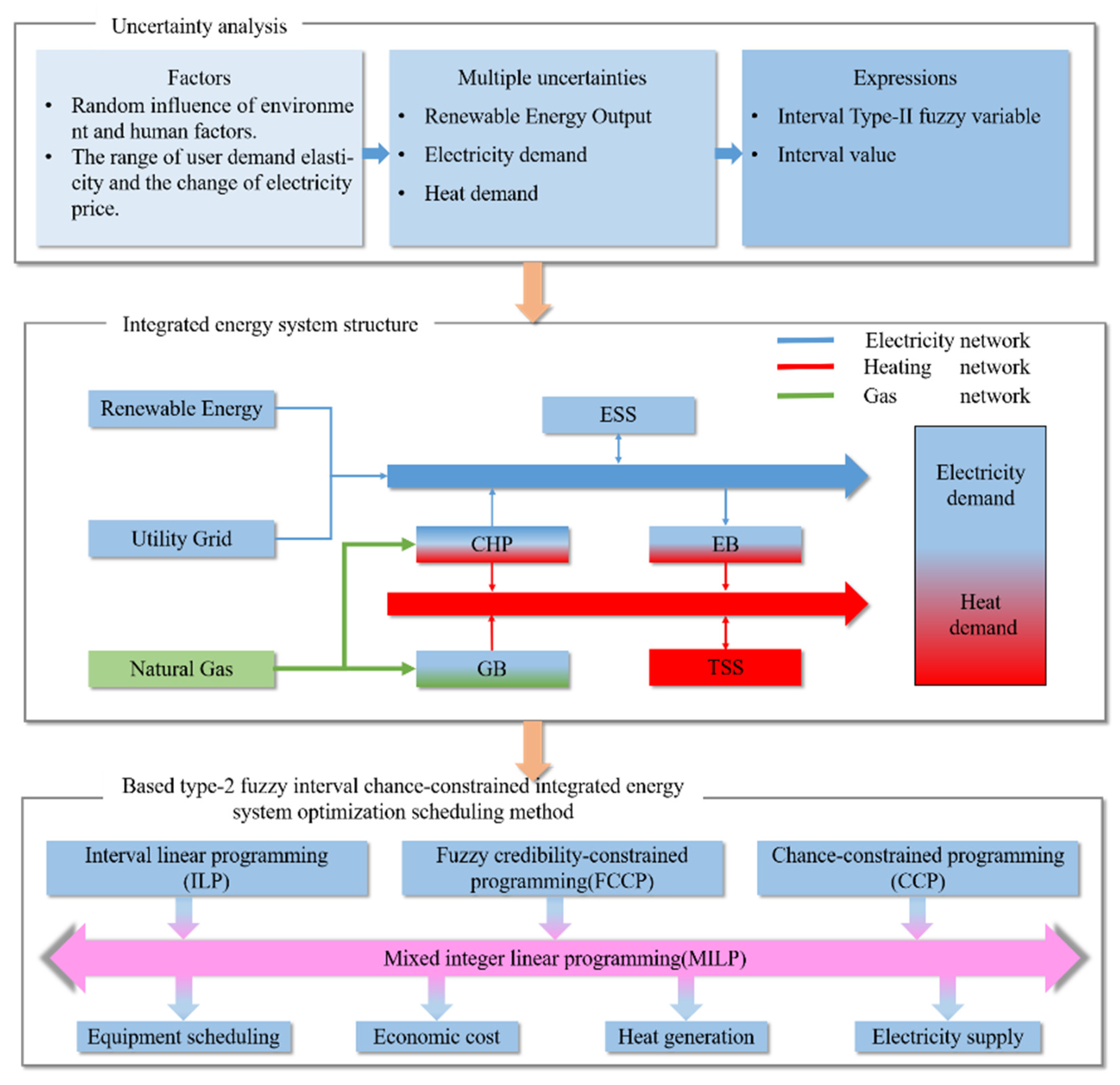
2. Problem Statement

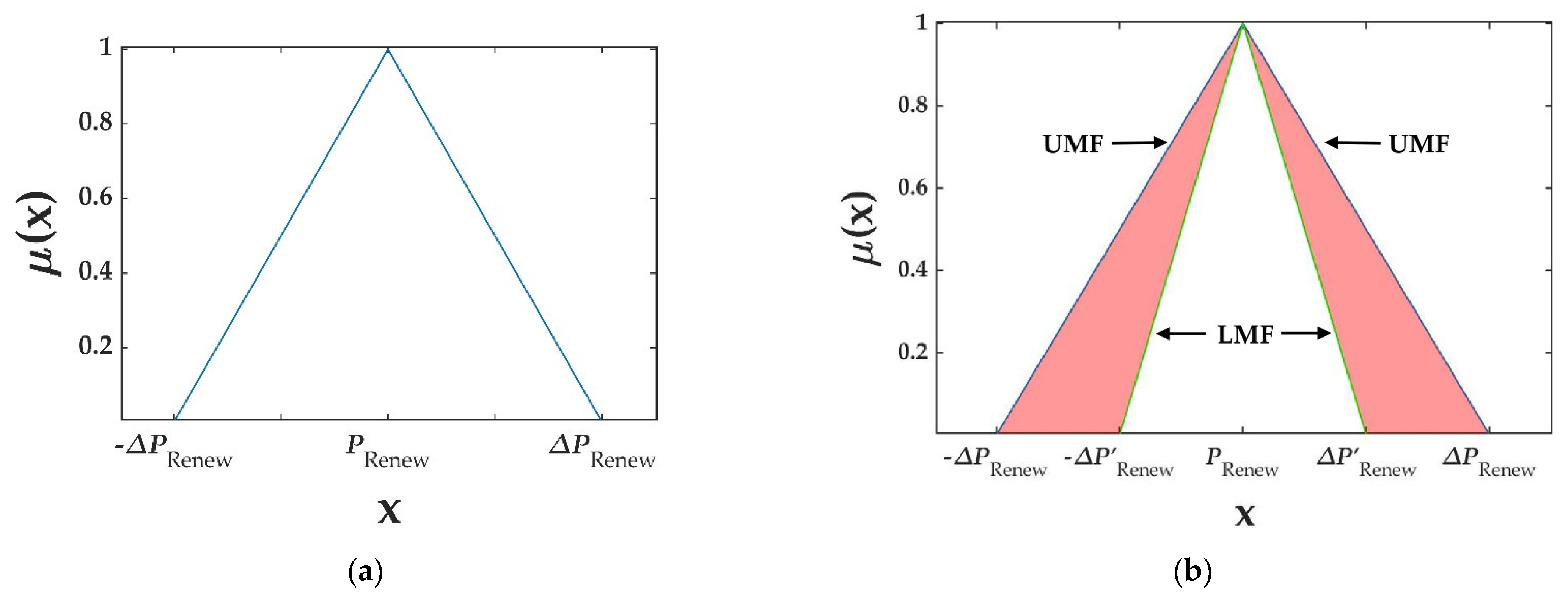
2.1. Renewable Energy Multiple Uncertainty Description

The uncertainty of RES mainly considers the intermittence, volatility, and prediction error of RES output. On the one hand, the output of RES is easily affected by environmental factors; on the other hand, different scholars have different ways to deal with the output data of RES. As a result, the prediction error of RES output power is also different [27]. According to different prediction errors, when describing them with fuzzy sets, the choice of MF may be different [28,29], which will affect the optimal scheduling results of the IES. The MF in the type−I fuzzy set that is commonly used now is single-valued [30,31], which cannot describe the uncertainty in the selection of MF. In contrast, the interval type-II fuzzy set expresses the affiliation degree of the type−I fuzzy set as a fuzzy set, and its type-II MF has a multivalued nature. Compared with the type−I MF, the type-II MF is more inclusive to the uncertainty [32], so the interval type-II fuzzy set is used to describe the uncertainty of RES output. Figure 1 shows the fuzzy description of RES, in which Figure 1a represents type−I MF, and Figure 1b represents type-II MF. It can be seen from the figure that the type−I MF is a single-valued function, so it can only describe a single uncertainty. The type-II MF, which is a multivalued function, is composed of infinite type−I MFs, so it can describe the multiple uncertainties of living energy.
In Figure 1b, footprint of uncertainty (FOU) represents the maximum uncertainty range of RES output power, which is composed of upper membership function (UMF) and lower membership function (LMF). FOU [29] is shown in Equation (1):
μ Renew ˜ ( x ) = { x P Renew + Δ P Renew Δ P Renew , P Renew Δ P Renew < x < P Renew 1 x = P Renew P Renew + Δ P Renew x Δ P Renew , P Renew < x P Renew + Δ P Renew 0   otherwise
where x represents the fuzzy variable of RES; μ Renew ˜ is a representative of RES type-II MF; P Renew represents the predicted output power of RES; and Δ P Renew and Δ P Renew represent the prediction error of RES.

2.2. Load Uncertainty Description

Compared with RES, the uncertainty of load is directly related to the elasticity of user demand and the change of electricity price; it often has certain rules to follow, so the accuracy of load forecasting is often higher than that of RES [33]. Compared with other description methods, the interval method can effectively avoid the errors caused by artificial subjective factors and make the uncertain information not easy to be lost in the process of the solution, and it is also easy to realize in engineering applications [34]. Therefore, this paper uses interval numbers to describe the predicted values of thermal and electrical loads, as shown in Equations (2) and (3):
P Eload ± = P Eload [ 1 α e , 1 + α e ] , α e [ 0 , 1 ]
P Hload ± = P Hload [ 1 α h , 1 + α h ] , α h [ 0 , 1 ]
P Eload ± and P Hload ± are the heat and electricity load of the building, respectively; α h and α e are the relative error range of thermal and electrical load forecasting, respectively.

3. Optimal Scheduling Method of IES Based on T2FICCP

The IES in this paper is connected to the utility grid and gas grid. The system mainly includes photovoltaic (PV) devices, combined heat and power (CHP) units, an electricity storage system (ESS), a thermal storage system (TSS), a gas boiler (GB), an electric boiler (EB), and other equipment units, as well as building heat and electricity load.
A T2FICCP optimization model is proposed to achieve accurate modeling of multiple uncertainties in RES for different uncertainty characteristics of the source-load side in the IES. It is based on three different optimization models, FCCP, ILP, and CCP, since each optimization model has its unique contribution to the treatment of uncertainty information in the system. For example, FCCP can solve the uncertainty problem in the system containing fuzzy information [35]; ILP can solve the uncertainty problem in the system expressed in the form of interval numbers [36]; and CCP can effectively reflect the reliability of satisfying system constraints under uncertainty [37]. In this paper, the above three optimization models are integrated into the MILP framework. Compared with the above optimization models, T2FICCP can simultaneously deal with multiple uncertainty problems containing type-II fuzzy sets as well as interval numbers’ descriptions in the system constraints and proposes an IES optimal scheduling method based on T2FICCP, with a basic framework that is shown in Figure 2.

3.1. Objective Function

Taking the above IES as the research object, the objective function of the T2FICCP model is set as the minimum comprehensive operating cost in a scheduling cycle, as shown in Equation (4):
min   C total ± = C E ± + C CHP ± + C GB ± + C ESS ±
where C total ± budget is the total operating cost of IES in one scheduling cycle. C E ± is the cost of purchasing electricity from utility grids. C CHP ± is the start-up, shutdown and operation cost of CHP units. C GB ± is the running cost of GB. C ESS ± is the running cost of ESS.
The cost of purchasing electricity from the utility grid is shown in Equation (5) [38]:
C E ± = i = 1 T P Grid ± ( i ) c Grid ( i ) Δ t
where i is the specific time step of scheduling, T is the number of periods of a single scheduling cycle, which can be set to 24 for day-ahead scheduling. P Grid ± ( i ) and c Grid ( i ) are the number of intervals and the price of power purchased from the utility grid in the i th time step, respectively. Δ t is the scheduling time step.
The start-up, stopping, and operating costs of the CHP unit are shown in Equation (6):
C CHP ± = S U , D CHP ( | δ CHP ( 1 ) B | + i = 2 T ( | δ CHP ( i 1 ) δ CHP ( i ) | ) ) + i = 1 T ( ( a P CHP ± ( i ) + b H CHP ± ( i ) + c δ CHP ( i ) ) Δ t )
where S U , D CHP is the cost of starting or shutting down a CHP unit once. B is the state variable of the CHP unit for the last period of the day before the schedule date. δ CHP ( i ) is the binary variable of the operating status of the CHP unit in the i th time step. P CHP ± ( i ) and H CHP ± ( i ) are the number of intervals of power generation and heat production of CHP units in the i th time step, respectively. a, b, and c are the linear cost factors of fuel for CHP units.
The GB operating cost is shown in Equation (7):
C GB ± = i = 1 T ( c g a s H GB ± ( i ) η G B Δ t )
where c gas is the unit calorific value price of natural gas. η G B is the GB heat production efficiency. H GB ± ( i ) is the number of intervals of GB heat production power in the i th time step.
The ESS operating cost is shown in Equation (8):
C ESS ± = c r i = 1 T ( ( δ E S S , c ( i ) P E S S , c ± ( i ) + δ E S S , d ( i ) P E S S , d ± ( i ) ) 1 C E S S _ c a p Δ t )
where c r is the cost of a single full charge/discharge. δ E S S , c ( i ) and δ E S S , d ( i ) are the binary variables of the ESS charge/discharge states in the i th time step, respectively. P E S S , c ± ( i ) and P E S S , d ± ( i ) are the number of intervals of ESS charging/discharging power in the i th time step, respectively. C ESS _ cap is the ESS capacity.

3.2. Constraint Condition

In this paper, the constraints of the optimal schedule model are set considering the source-load uncertainty in the system, power and heat balance, CHP units, energy storage system, GB, EB, and power constraints between the contact line with the grid.
  • IES Power Constraints
The IES power constraint includes the balance constraint of electric power and thermal power. Compared with the electric power balance of the conventional model, the electric power balance constraint in this paper requires interval fuzzy treatment, considering that the system contains both PV uncertainty described by a type-II fuzzy set and load uncertainty described by interval numbers. Since the supply and demand of thermal power in the model do not necessarily need to be balanced at all times, the thermal power balance constraint is described by fuzzy equivalence in this paper. The balance constraints for electric and thermal power are shown in Equations (9) and (10), respectively:
C ˜ r { P Grid ± ( i ) + P CHP ± ( i ) + δ ESS , c ( i ) P ESS , c ± ( i ) δ ESS , d ( i ) P ESS , d ± ( i ) + m = 1 M P e , load ± ( m , i ) P e , EB ± ( i ) P Renew ( i ) } β
H CHP ± ( i ) + δ TSS , c ( i ) H TSS , c ± ( i ) δ TSS , d ( i ) H TSS , d ± ( i ) + η EB P e , EB ± ( i ) + H G B ± ( i ) = ˜ m = 1 M H h , load ± ( m , i ) + H h , loss ± ( i )
where C ˜ r { } is the fuzzy confidence level that the constraint holds. β is the given confidence level. P e , E B ± ( i ) and P e , l o a d ± ( m , i ) are the EB input power in the i th time step and the number of electrical load intervals in the m th building, respectively. P Renew ( i ) is the interval type-II fuzzy number of PV power generation in the i th time step, with a specific form that is given in Equation (1). δ T S S , c ( i ) and δ TSS , d ( i ) are the binary variables of the TSS charging and discharging heat state in the i th time step, respectively. H TSS , c ± ( i ) and H TSS , d ± ( i ) are the number of intervals of TSS charging and discharging thermal power in the i th time step, respectively. η E B is the heat production efficiency of the EB. H h , l o a d ± ( m , i ) and H h , loss ± ( m , i ) are the number of heat load intervals and the number of total heat loss power intervals of the building for the m th building in the i th time step, respectively.
2.
CHP Unit Operating Constraints
The power generated and heat produced by the CHP unit must satisfy its operating characteristic constraints as well as the uphill and downhill power constraints, with constraint equations that are shown in Equations (11) and (12):
{ max { c λ 2 H CHP ± ( i ) + P CHP min , λ ( H CHP ± ( i ) H 0 ) } P CHP ± ( i ) c λ 1 H CHP ± ( i ) + P C H P max 0 H CHP ± ( i ) H C H P max
where P C H P min and P C H P max are the maximum and minimum values of the power generated by the CHP unit under pure condensing conditions, respectively. H C H P max is the maximum heat production power of the CHP unit. c λ 1 and c λ 2 are the slopes of the curves for condensing units. λ is the slope of the curve for back-pressure units. H 0 is the heat threshold at which steam from a back-pressure unit drives the turbine to do work.
{ | P C H P ± ( 1 ) P C H P ( B ) | Δ P U , D Δ t | H C H P ± ( 1 ) H C H P ( B ) | Δ H U , D Δ t { | P C H P ± ( i ) P C H P ( k 1 ) | Δ P U , D Δ t | H C H P ± ( i ) H C H P ( k 1 ) | Δ H U , D Δ t , k 2
where P C H P ( B ) and H C H P ( B ) are the electric power and thermal power of the CHP unit at the last moment of the day-ahead schedule, respectively. Δ P U , D and Δ H U , D are the maximum changes of power generation and heat production power of CHP unit per unit time, respectively.
3.
ESS Energy Storage Constraints
ESS constraints mainly include capacity constraints and charging/discharging power constraints, as shown in Equations (13) and (14):
{ S S O C ± ( 1 ) = S S O C ( B ) ( 1 σ E S S ) + ( η E S S δ E S S , c ( 1 ) P E S S , c ± ( 1 ) δ E S S , d ( 1 ) P E S S , d ± ( 1 ) / η E S S ) Δ t C E S S _ c a p S S O C ± ( i ) = S S O C ± ( i 1 ) ( 1 σ E S S ) + ( η E S S δ E S S , c ( i ) P E S S , c ± ( i ) δ E S S , d ( i ) P E S S , d ± ( i ) / η E S S ) Δ t C E S S _ c a p , i 2 δ E S S , c ( i ) + δ E S S , d ( i ) ( 0 , 1 ) S S O C min S S O C ± ( i ) S S O C max
where S S O C ± ( i ) is the number of storage capacity intervals of the ESS in the i th time step. S S O C ( B ) is the storage capacity of ESS at the last moment of day-ahead scheduling. σ E S S and η E S S are the storage system self-discharge efficiency and ESS charge/discharge efficiency, respectively. S S O C min and S S O C max are the maximum and minimum storage capacities of the ESS, respectively.
P E S S c , d , m i n δ E S S , c ( i ) P E S S , c ± ( i ) + δ E S S , d ( i ) P E S S , d ± ( i ) P E S S c , d , m a x
where P E S S c , d , m i n and P E S S c , d , m a x are the maximum and minimum charge/discharge powers, respectively.
4.
TSS Energy Storage Constraints
The TSS constraints mainly include capacity constraints and charging/discharging power constraints, and the main constraint equations are shown in Equations (15) and (16):
{ S S O T ± ( 1 ) = S S O T ( B ) ( 1 σ T S S ) + ( η T S S δ T S S , c ( 1 ) H T S S , c ± ( 1 ) δ T S S , d ( 1 ) H T S S , d ± ( 1 ) / η T S S ) Δ t C T S S _ c a p S S O T ± ( i ) = S S O T ± ( i 1 ) ( 1 σ S O T ) + ( η T S S δ T S S , c ( i ) H T S S , c ± ( i ) δ T S S , d ( i ) H T S S , d ± ( i ) / η T S S ) Δ t C T S S _ c a p , i 2 δ T S S , c ( i ) + δ T S S , d ( i ) ( 0 , 1 ) S S O T min S S O T ± ( i ) S S O T max
where S S O T ± ( i ) is the number of storage capacity intervals of TSS in the i th time step. S S O T ( B ) is the storage capacity of TSS at the last moment of day-ahead scheduling. σ T S S and η T S S are the storage system self-discharge efficiency and TSS charge/discharge efficiency, respectively. C T S S _ c a p is the TSS capacity. S S O T min and S S O T max are the maximum and minimum storage capacities of ESS, respectively.
H T S S c , d , m i n δ T S S , c ( i ) H T S S , c ± ( i ) + x T S S , d ( i ) H T S S , d ± ( i ) H T S S c , d , m a x
where P T S S c , d , m i n and P T S S c , d , m a x are the maximum and minimum charge/discharge powers, respectively.
5.
GB, EB, and Utility Grid Contact Line Power Constraints
{ 0 H G B ± ( i ) H G B max 0 P e , E B ± ( i ) P E B max 0 P G r i d ± ( i ) P G r i d max
where H G B max is the maximum heat production power of GB. P E B max is the maximum EB input power. P G r i d max is the maximum purchased power of the IES.

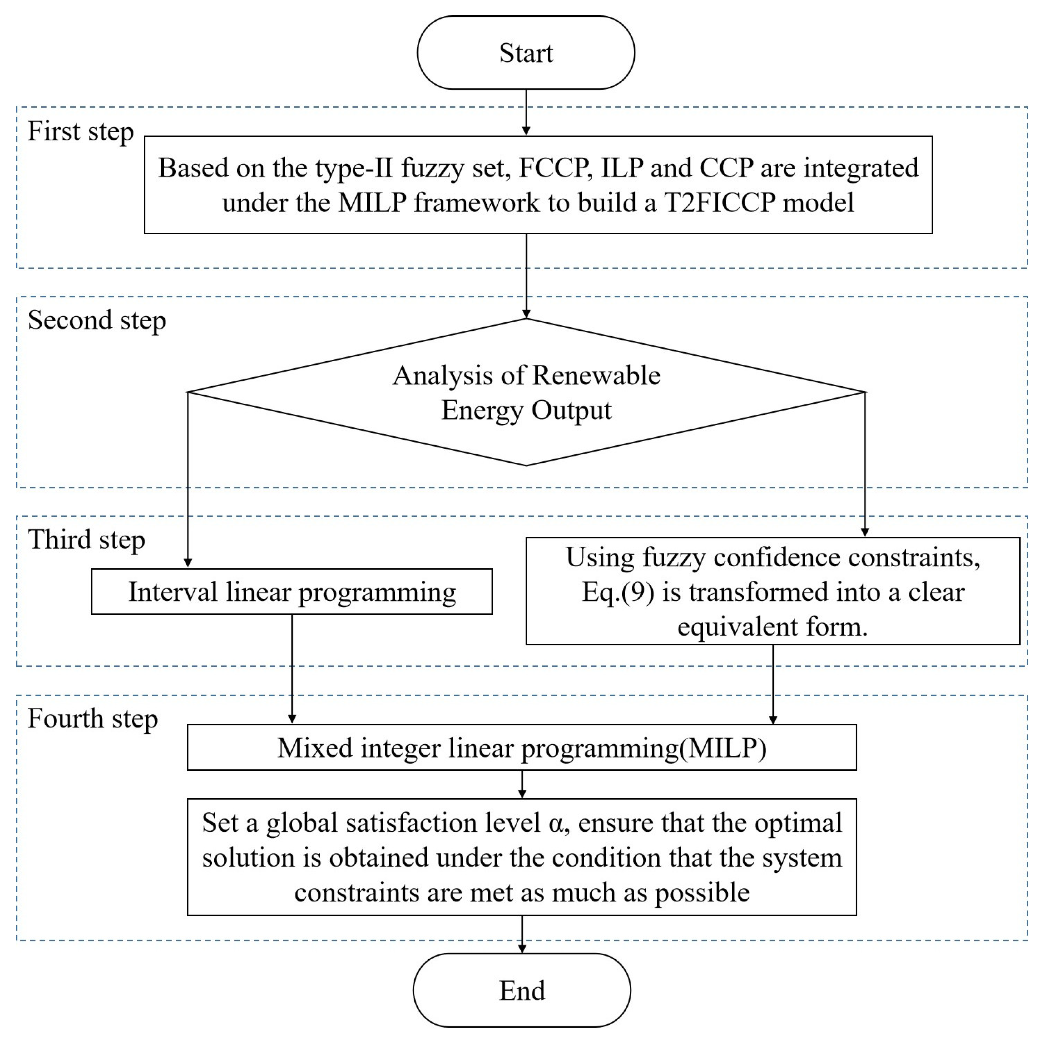
3.3. Hybrid Solving Algorithm Based on ILP and T2FICCP

For the intermittent characteristics of PV, a hybrid solution algorithm based on ILP and T2FICCP is used to solve the problem, as shown in Figure 3. Specifically, the ILP optimization model can simplify the model and improve the calculation speed when solving during the time without PV output, such as night or rainy days; and the T2FICCP optimization model can reduce the dependence on uncertainty factors and make the scheduling results more realistic and reliable by accurately modeling and solving the multiple uncertain information in the IES when PV output is available. The steps are shown as follows.
Step 1: type-II fuzzy sets are used to describe RES uncertainty, and interval numbers are used to describe load uncertainty, while the T2FICCP model is constructed by integrating FCCP, ILP, and CCP under the MILP framework based on type-II fuzzy sets.
Step 2: different optimization models are used to classify the solution considering the PV output condition. In the PV non-output hours or less hours, the ILP solution is used; in the PV output hours, the T2FICCP solution is used to convert the type-II fuzzy set into a clear equivalent form using fuzzy credibility constraints and construct two CCP submodels using generalized credibility, and then the two CCP models are converted into deterministic models [39].
Step 3: the deterministic model in the second step is combined with the ILP and made to decompose into an upper bound submodel and a lower bound submodel, and the optimal solutions of the two submodels are found to obtain an optimal solution interval.
Step 4: a confidence level is set, and an optimal solution that maximally satisfies the system constraints is sought within the optimal solution interval found in the third step.
Step 5: a confidence level α is set, and an optimal solution that maximally satisfies the system constraints is sought within the optimal solution interval found in the third step.

4. Simulation Research

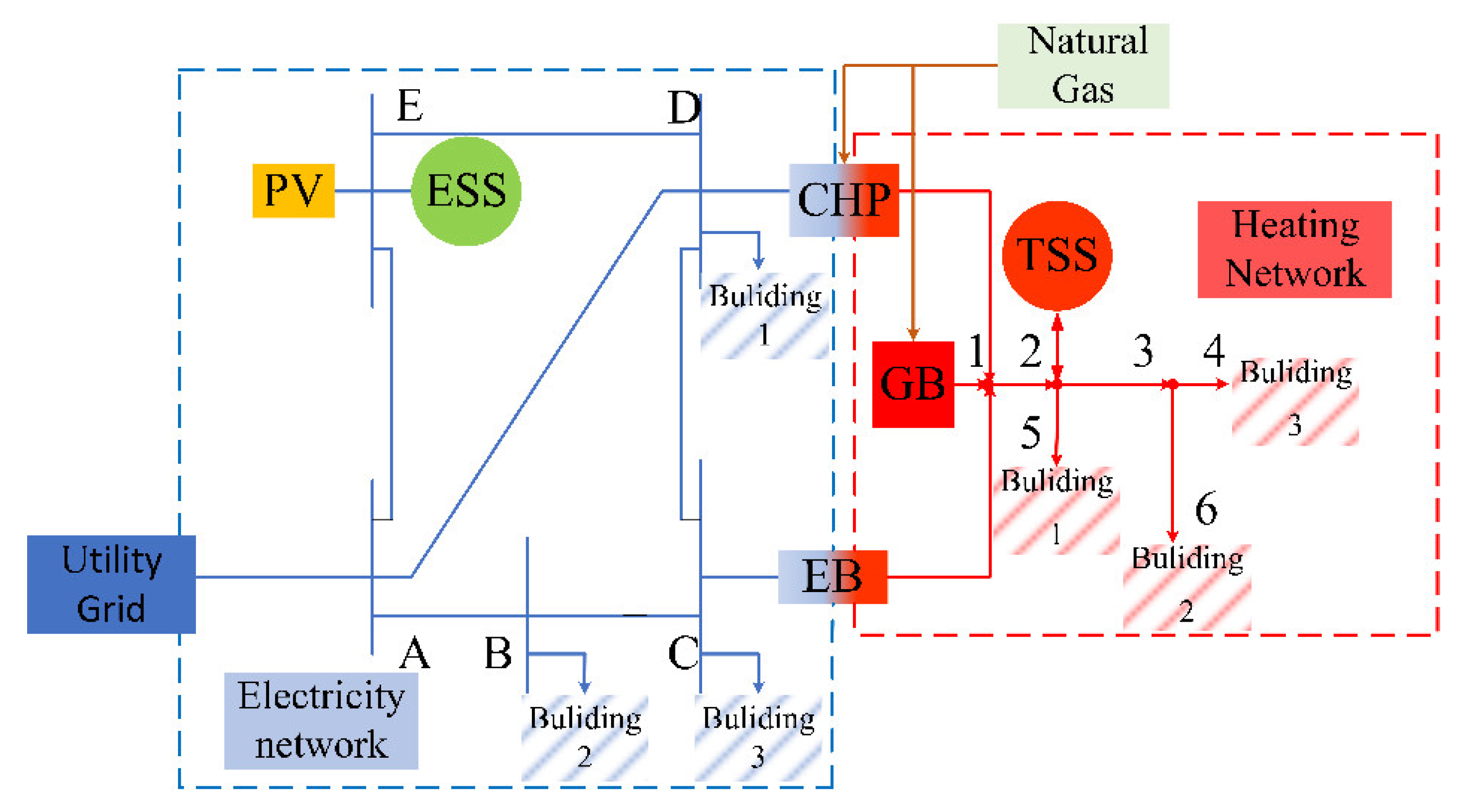
4.1. System Infrastructure and Data Sources

The IES studied in this paper is constructed by referring to the PJM five-bus electrical network structure and the six-node thermal network model in Ref. [40], as shown in Figure 4. Bus A is connected to the main grid, EB is installed at Bus C, unit CHP is connected to the power grid at Bus D, and both PV and ESS are installed at Bus E. In the thermal network, Bus 1 connects with CHP, EB, and GB. The electric load and thermal load are distributed at Bus B, C, and D and Bus 4, 5, and 6.
Since microgrids generally have short physical distances, the power losses in microgrids can be neglected. The thermal network loss parameters and TSS loss parameters are given in Ref. [40]; the operating characteristics of CHP units are shown in Figure A1 (in Appendix A); the operating parameters of CHP and ESS are shown in Table A1 [40,41]. In order to verify the effectiveness of the method in different seasons and different weather, this paper simulates 20 days (5 sunny days and 5 cloudy days in both summer and winter) of PV power prediction data, as well as load prediction data, to derive the statistical results of the IES schedule cost. These 20 days are named as summer sunny days 1–5 (SSday1–5), summer cloudy days 1–5 (SCday1–5), winter sunny days 1–5 (WSday1–5), and winter cloudy days 1–5 (WCday1–5), and the corresponding PV predicted output power curves are shown in Figure 5. The PV predicted output power data in this paper are from Hangzhou Dianzi University’s PV microgrid system; the thermal and electrical load prediction data of typical buildings are from San Francisco, CA, USA, provided by the website of the U.S. Energy Agency; the purchased power price and natural gas unit calorific value price are provided by the website of PG&E.

4.2. Simulation Results and Analysis

In order to verify the statistical effectiveness of the proposed T2FICCP-based day-ahead scheduling model, two other related models are introduced in this paper, and the three models are simulated and compared for experiments. The compared models can be listed as:
Uncertainty model-1: type−I fuzzy set is used to describe PV uncertainty and interval numbers are used to describe load uncertainty, which is solved using fuzzy interval confidence planning.
Uncertainty model-2: type-II fuzzy set is used to describe PV uncertainty as well as load uncertainty, which is solved using type-II fuzzy confidence planning.
T2FICCP model (proposed in this paper): the type-II fuzzy set is used to describe the PV output power uncertainty and the interval numbers are used to describe the load uncertainty, which is solved using a hybrid solution algorithm.
Taking four typical days of SSday-1, SCday-4, WSday-1, and WCday-1 as examples, the scheduling costs for a typical summer and winter day, β = 0.95, are given in Table 1. From the comparison of different methods, the model proposed in this paper has the best scheduling cost value. The cost comparison with model-1 shows that this paper uses the type-II fuzzy set to express PV uncertainty, and the uncertainty of PV output is better described by the type-II fuzzy set than the type−I fuzzy set. Model-2 does not take into account the difference between PV and load uncertainty characteristics, so the scheduling effect is not as good as the proposed method.
Comparing different seasons and different weather types, the schedule cost is lower on sunny days than on cloudy days and is lower in summer than in winter. This is due to the smoother PV output on sunny days, and the smaller load and larger PV generation in summer compared to winter. Figure 6 gives the scheduling plan of the proposed method, β = 0.95, with SSday-1 as an example. It can be seen from the figure that during the low electricity price and low building load hours, the grid-purchased electricity and GB heating meet the load requirements. When the building load increases to a certain value, the CHP unit starts to meet the load requirements while charging and charging the ESS and TSS with heat. After sunrise, the PV output gradually increases, the CHP unit will stop working, and the ESS and TSS start discharging and discharging heat. It can be seen that the IES integrates multiple energy sources and energy-using devices, giving full play to their complementary advantages in terms of operating characteristics and operating costs in the time domain, realizing the coordinated optimization of multiple energy outputs.
In this paper, we also simulate the IES scheduling with different confidence levels. Taking a cloudy day SCday-4 in summer as an example, Table 2 gives the scheduling costs of different methods with different confidence levels for the same prediction error. From the cross-sectional comparison, the proposed method gives the lowest cost scheduling solution regardless of the confidence level, with model-1 being the second-lowest and model-2 being the highest. This is because the proposed method models uncertainty more accurately and uses a hybrid solution algorithm, which makes the scheduling cost better. From the vertical view, as the confidence level increases, the operational reliability of the IES increases, but the operational cost increases, which is in line with the general rule that reliability and economy are mutually exclusive.
In this paper, IES scheduling with different prediction errors is simulated. Taking a cloudy day SCday-4 in summer as an example, Table 3 shows the different scheduling costs for the same confidence level with different load forecasting errors. From the cross-sectional comparison, the proposed method has the best scheduling cost regardless of the error level. This is due to the fact that the proposed T2FICCP model models the uncertainty more accurately and reduces the dependence on the prediction accuracy. Longitudinally, the scheduling cost of all models gradually increases as the load forecasting error gradually increases, but the proposed method has less fluctuation compared with model-1. This is due to the fact that the interval method can effectively avoid the errors caused by human subjective factors and simplify the uncertain information to a certain extent. Table 4 gives the different scheduling costs for different PV power prediction errors at the same confidence level. From the longitudinal comparison, as the PV power prediction error gradually increases, the scheduling cost of all models gradually increases, but the proposed method fluctuates less with model-2. This is because the type-II fuzzy set is better than the type−I fuzzy set in dealing with uncertainty.

5. Conclusions

Aiming at the multiple uncertainties of RES generation and load in the IES, this paper proposes an IES day-ahead economic scheduling model based on T2FICCP to solve the impact of multiple uncertainties on IES scheduling. In addition, through the simulation verification of the case, the following conclusions can be obtained.
  • Compared with the traditional fuzzy and interval optimization models, the T2FICCP optimization model describes the uncertainty more comprehensively and uses different methods to describe the uncertain information according to the different uncertainty characteristics; the economic cost is better than other optimization models, which shows that the performance of T2FICCP when dealing with multiple uncertainties is better.
  • In this paper, according to the intermittent characteristics of RES, a hybrid algorithm is adopted. Compared with the traditional algorithm, it can effectively reduce the dependence on uncertain factors, make the scheduling results more real and reliable, and improve the computing speed.
  • The operation cost of the IES changes with the prediction accuracy, confidence level, and load prediction error, which reflects the dynamic fluctuation of the IES to the prediction error.
  • This research mainly compares the operating costs of RES and load forecast errors at different confidence levels, and gives the IES scheduling plan under the optimal operating cost. The research results show that the model proposed in this paper can effectively improve the capacity of IES to consume RES, give full play to the complementary advantages of operating characteristics and operating costs of multiple energy sources and energy-using equipment, and realize the coordinated optimization of multiple energy output.
As mentioned in the Section 2, this paper only describes the multiple uncertainties on the source-load side, but there will be different uncertainties in the operation of IES, such as CHP operating conditions, dynamic characteristics of the thermal network, and so on. We will further study this problem in the future. In addition, at present, many studies only focus on the time-domain characteristics of RES, but do not take into account the frequency-domain characteristics, so the description of RES is single, which is also the focus of our future research.

Author Contributions

Conceptualization, L.Z. and X.S.; methodology, X.S.; software, X.S.; validation, L.Z., X.S. and H.W.; investigation, S.G.; resources, X.S.; data curation, S.G.; writing—original draft preparation, X.S.; writing—review and editing, L.Z. and X.S.; visualization, H.W. All authors have read and agreed to the published version of the manuscript.

Funding

This research received no external funding.

Data Availability Statement

The data that support the findings of this study are available from the corresponding author upon reasonable request.

Acknowledgments

The authors would like to thank all the reviewers and the editors for their constructive comments and valuable suggestions that led to improvements in the quality of this paper.

Conflicts of Interest

The authors declare no conflict of interest.

Appendix A

Figure A1. The operation interval of CHP units.
Energies 15 06763 g0a1
Table A1. Device parameters.
DeviceSymbolValue
CHP c λ 1 −0.1778
c λ 2 −0.1698
λ 1.7819
P CHP max 600 kW
P CHP min 100 kW
H CHP max 500 kWth
H 0 213.167 kWth
B 0
a 3.45 × 10 8 USD/kW2
b 0.0145 USD/kW
c USD 64.37
d 3.0 × 10 8 USD/kWth2
e 0.0042 USD/kW
f 3.1 × 10 8 USD/kW-kWth
Δ P U , D 200 kW/h
Δ H U , D 200 kWth/h
S U , D CHP USD 10
ESS c r USD 7.1217
η ESS 0.99
P ESS c , d , max 200kW
P ESS c , d , min 0
S SOC max 0.9
S SOC min 0.1
S SOC ( B ) 0.1
c ESS _ cap 500 kWh
TSS η TSS 0.87
H TSS c , d , max 100 kWth
H TSS c , d , min 0
T TSS max 0.9
T TSS min 0.1
T TSS ( B ) 0.1
C TSS _ cap 500 kWth/h
GB η GB 0.9
H GB max 200 kWth
EB η EB 0.97
P EB max 150 kW
Grid P Grid max 300 kW
Figure A2. Building electricity/thermal load forecast curve for the case study.
Energies 15 06763 g0a2
Figure A3. Electricity purchase price and natural gas price for the summer and winter days.
Energies 15 06763 g0a3

References

  1. Gao, Q.; Zhang, X.; Yang, M.; Chen, X.; Zhou, H.; Yang, Q. Fuzzy Decision-Based Optimal Energy Dispatch for Integrated Energy Systems With Energy Storage. Front. Energy Res. 2021, 9, 809024. [Google Scholar] [CrossRef]
  2. Wang, Y.; Yu, H.; Yong, M.; Huang, Y.; Zhang, F.; Wang, X. Optimal Scheduling of Integrated Energy Systems with Combined Heat and Power Generation, Photovoltaic and Energy Storage Considering Battery Lifetime Loss. Energies 2018, 11, 1676. [Google Scholar] [CrossRef]
  3. Zhang, Y.; He, Y.; Yan, M.; Guo, C.; Ding, Y. Linearized Stochastic Scheduling of Interconnected Energy Hubs Considering Integrated Demand Response and Wind Uncertainty. Energies 2018, 11, 2448. [Google Scholar] [CrossRef]
  4. Gao, J.; Yang, Y.; Gao, F.; Wu, H. Two-Stage Robust Economic Dispatch of Regional Integrated Energy System Considering Source-Load Uncertainty Based on Carbon Neutral Vision. Energies 2022, 15, 1596. [Google Scholar] [CrossRef]
  5. Wang, W.; Dong, H.; Luo, Y.; Zhang, C.; Zeng, B.; Xu, F.; Zeng, M. An Interval Optimization-Based Approach for Electric–Heat–Gas Coupled Energy System Planning Considering the Correlation between Uncertainties. Energies 2021, 14, 2457. [Google Scholar] [CrossRef]
  6. Zhou, C.; Huang, G.; Chen, J. A Type-2 Fuzzy Chance-Constrained Fractional Integrated Modeling Method for Energy System Management of Uncertainties and Risks. Energies 2019, 12, 2472. [Google Scholar] [CrossRef]
  7. Oh, U.; Lee, Y.; Choi, J.; Karki, R. Reliability evaluation of power system considering wind generators coordinated with multi-energy storage systems. IET Gener. Transm. Distrib. 2020, 14, 786–796. [Google Scholar] [CrossRef]
  8. Zhang, D.; Jiang, S.; Liu, J.; Wang, L.; Chen, Y.; Xiao, Y.; Jiao, S.; Xie, Y.; Zhang, Y.; Li, M. Stochastic Optimization Operation of the Integrated Energy System Based on a Novel Scenario Generation Method. Processes 2022, 10, 330. [Google Scholar] [CrossRef]
  9. Liu, G.; Starke, M.; Xiao, B.; Zhang, X.; Tomsovic, K. Microgrid optimal scheduling with chance-constrained islanding capability. Electr. Power Syst. Res. 2017, 145, 197–206. [Google Scholar] [CrossRef]
  10. Zhao, P.; Gu, C.; Huo, D.; Shen, Y.; Hernando-Gil, I. Two-Stage Distributionally Robust Optimization for Energy Hub Systems. IEEE Trans. Ind. Inform. 2020, 16, 3460–3469. [Google Scholar] [CrossRef]
  11. Zhang, Y.; Le, J.; Zheng, F.; Zhang, Y.; Liu, K. Two-stage distributionally robust coordinated scheduling for gas-electricity integrated energy system considering wind power uncertainty and reserve capacity configuration. Renew. Energy 2019, 135, 122–135. [Google Scholar] [CrossRef]
  12. Tan, Z.; Tan, Q.; Yang, S.; Ju, L.; De, G. A Robust Scheduling Optimization Model for an Integrated Energy System with P2G Based on Improved CVaR. Energies 2018, 11, 3437. [Google Scholar] [CrossRef]
  13. Li, Y.; Wang, K.; Gao, B.; Zhang, B.; Liu, X.; Chen, C. Interval optimization based operational strategy of integrated energy system under renewable energy resources and loads uncertainties. Int. J. Energy Res. 2020, 45, 3142–3156. [Google Scholar] [CrossRef]
  14. Aslam, S.; Khalid, A.; Javaid, N. Towards efficient energy management in smart grids considering microgrids with day-ahead energy forecasting. Electr. Power Syst. Res. 2020, 182, 106232. [Google Scholar] [CrossRef]
  15. Bai, L.; Li, F.; Cui, H.; Jiang, T.; Sun, H.; Zhu, J. Interval optimization based operating strategy for gas-electricity integrated energy systems considering demand response and wind uncertainty. Appl. Energy 2016, 167, 270–279. [Google Scholar] [CrossRef]
  16. Liu, H.; Tian, S.; Wang, X.; Cao, Y.; Zeng, M.; Li, Y. Optimal Planning Design of a District-Level Integrated Energy System Considering the Impacts of Multi-Dimensional Uncertainties: A Multi-Objective Interval Optimization Method. IEEE Access 2021, 9, 26278–26289. [Google Scholar] [CrossRef]
  17. Li, Z.; Zhang, Z. Day-Ahead and Intra-Day Optimal Scheduling of Integrated Energy System Considering Uncertainty of Source & Load Power Forecasting. Energies 2021, 14, 2539. [Google Scholar] [CrossRef]
  18. Zhou, C.; Huang, G.; Chen, J. A Multi-Objective Energy and Environmental Systems Planning Model: Management of Uncertainties and Risks for Shanxi Province, China. Energies 2018, 11, 2723. [Google Scholar] [CrossRef]
  19. Doan, A.T.; Viet, D.T.; Duong, M.Q. Economic load dispatch solutions considering multiple fuels for thermal units and generation cost of wind turbines. Int. J. Electr. Comput. Eng. 2021, 11, 3718–3726. [Google Scholar] [CrossRef]
  20. Waseem, M.; Lin, Z.; Liu, S.; Zhang, Z.; Aziz, T.; Khan, D. Fuzzy compromised solution-based novel home appliances scheduling and demand response with optimal dispatch of distributed energy resources. Appl. Energy 2021, 290, 116761. [Google Scholar] [CrossRef]
  21. Liu, X.; Xie, S.; Geng, C.; Yin, J.; Xiao, G.; Cao, H. Optimal Evolutionary Dispatch for Integrated Community Energy Systems Considering Uncertainties of Renewable Energy Sources and Internal Loads. Energies 2021, 14, 3644. [Google Scholar] [CrossRef]
  22. Guo, X.; Gong, R.; Bao, H.; Wang, Q. Hybrid Stochastic and Interval Power Flow Considering Uncertain Wind Power and Photovoltaic Power. IEEE Access 2019, 7, 85090–85097. [Google Scholar] [CrossRef]
  23. Liu, Z.; Huang, G.; Li, W. An inexact stochastic–fuzzy jointed chance-constrained programming for regional energy system management under uncertainty. Eng. Optim. 2014, 47, 788–804. [Google Scholar] [CrossRef]
  24. Mohammadi, M.; Noorollahi, Y.; Mohammadi-ivatloo, B. Fuzzy-based scheduling of wind integrated multi-energy systems under multiple uncertainties. Sustain. Energy Technol. Assess. 2020, 37, 100602. [Google Scholar] [CrossRef]
  25. Zhen, J.L.; Huang, G.H.; Li, W.; Liu, Z.P.; Wu, C.B. An inexact optimization model for regional electric system steady operation management considering integrated renewable resources. Energy 2017, 135, 195–209. [Google Scholar] [CrossRef]
  26. Wang, K.; Qi, X.; Liu, H. Photovoltaic power forecasting-based LSTM-Convolutional Network. Energy 2019, 189, 116225. [Google Scholar] [CrossRef]
  27. Han, S.; Qiao, Y.-H.; Yan, J.; Liu, Y.-Q.; Li, L.; Wang, Z. Mid-to-long term wind and photovoltaic power generation prediction based on copula function and long short term memory network. Appl. Energy 2019, 239, 181–191. [Google Scholar] [CrossRef]
  28. Yin, J.; Zhao, D. Fuzzy Stochastic Unit Commitment Model with Wind Power and Demand Response under Conditional Value-At-Risk Assessment. Energies 2018, 11, 341. [Google Scholar] [CrossRef]
  29. Mendel, J.M.; John, R.I. Type-2 fuzzy sets made simple. IEEE Trans. Fuzzy Syst. 2001, 10, 117–127. [Google Scholar] [CrossRef]
  30. Guerrero, J.M.; Chandorkar, M.; Lee, T.-L.; Loh, P.C. Advanced Control Architectures for Intelligent Microgrids-Part I: Decentralized and Hierarchical Control. IEEE Trans. Ind. Electron. 2013, 60, 1254–1262. [Google Scholar] [CrossRef] [Green Version]
  31. Khalid, R.; Javaid, N.; Rahim, M.H.; Aslam, S.; Sher, A. Fuzzy energy management controller and scheduler for smart homes. Sustain. Comput. Inform. Syst. 2019, 21, 103–118. [Google Scholar] [CrossRef]
  32. Siahkali, H.; Vakilian, M. Interval type-2 fuzzy modeling of wind power generation in Genco’s generation scheduling. Electr. Power Syst. Res. 2011, 81, 1696–1708. [Google Scholar] [CrossRef]
  33. Mamun, A.A.; Sohel, M.; Mohammad, N.; Haque Sunny, M.S.; Dipta, D.R.; Hossain, E. A Comprehensive Review of the Load Forecasting Techniques Using Single and Hybrid Predictive Models. IEEE Access 2020, 8, 134911–134939. [Google Scholar] [CrossRef]
  34. Ji, L.; Niu, D.X.; Xu, M.; Huang, G.H. An optimization model for regional micro-grid system management based on hybrid inexact stochastic-fuzzy chance-constrained programming. Int. J. Electr. Power Energy Syst. 2015, 64, 1025–1039. [Google Scholar] [CrossRef]
  35. Liu, J.; Nie, S.; Shan, B.G.; Li, Y.P.; Huang, G.H.; Liu, Z.P. Development of an interval-credibility-chance constrained energy-water nexus system planning model—A case study of Xiamen, China. Energy 2019, 181, 677–693. [Google Scholar] [CrossRef]
  36. Li, Y.P.; Nie, S.; Huang, C.Z.; McBean, E.A.; Fan, Y.R.; Huang, G.H. An Integrated Risk Analysis Method for Planning Water Resource Systems to Support Sustainable Development of an Arid Region. J. Environ. Inform. 2017, 29, 1–15. [Google Scholar] [CrossRef]
  37. Kundu, P.; Majumder, S.; Kar, S.; Maiti, M. A method to solve linear programming problem with interval type-2 fuzzy parameters. Fuzzy Optim. Decis. Mak. 2018, 18, 103–130. [Google Scholar] [CrossRef]
  38. Zheng, L.; Zhou, X.; Qiu, Q.; Yang, L. Day-ahead optimal dispatch of an integrated energy system considering time-frequency characteristics of renewable energy source output. Energy 2020, 209, 118434. [Google Scholar] [CrossRef]
  39. Li, G.; Zhang, R.; Jiang, T.; Chen, H.; Bai, L.; Cui, H.; Li, X. Optimal dispatch strategy for integrated energy systems with CCHP and wind power. Appl. Energy 2017, 192, 408–419. [Google Scholar] [CrossRef]
  40. Jin, M.; Feng, W.; Liu, P.; Marnay, C.; Spanos, C. MOD-DR: Microgrid optimal dispatch with demand response. Appl. Energy 2017, 187, 758–776. [Google Scholar] [CrossRef] [Green Version]
  41. Divya, K.C.; Østergaard, J. Battery energy storage technology for power systems—An overview. Electr. Power Syst. Res. 2009, 79, 511–520. [Google Scholar] [CrossRef]
Figure 1. Fuzzy membership function. (a) Type−I membership function. (b) Type-II membership function.
Energies 15 06763 g001
Figure 2. Optimal scheduling framework of IES based on T2FICCP.
Energies 15 06763 g002
Figure 3. Flow chart of hybrid solution algorithm.
Energies 15 06763 g003
Figure 4. The IES network structure.
Energies 15 06763 g004
Figure 5. PV power generation prediction curves.
Energies 15 06763 g005
Figure 6. The operation plan of model 3 on the typical day of SSday-1 (β = 0.95).
Energies 15 06763 g006
Table 1. Scheduling costs of different models for the same typical day (β = 0.95).
Typical DaysModel-1 (USD)Model-2 (USD)T2FICCP (USD)
SSday-11273.61276.11254.9
SCday-41285.41288.11267.3
WSday-11329.31334.51315.8
WCday-11342.61348.71329.6
Table 2. Schedule costs for a typical day of SCday-4 at different confidence levels (PV power as well as load prediction errors are constant).
βModel-1 (USD)Model-2 (USD)T2FICCP (USD)
0.951285.41288.11271.9
0.91283.81285.91271.1
0.851282.11283.71270.6
0.81280.31281.61270.1
Table 3. Scheduling costs for different load prediction errors (β = 0.95, constant PV power prediction error).
Load Prediction ErrorModel-1 (USD)Model-2 (USD)T2FICCP (USD)
0.051278.11288.11271.9
0.11290.71299.81275.1
0.151302.31327.51305.6
0.21316.11346.31310.2
Table 4. Scheduling costs for different PV prediction errors (β = 0.95, constant load prediction error).
PV Prediction ErrorModel-1 (USD)Model-2 (USD)T2FICCP (USD)
0.051278.11288.11271.9
0.11281.91289.11274.1
0.151284.51290.51277.1
0.21289.11292.11280.1
Publisher’s Note: MDPI stays neutral with regard to jurisdictional claims in published maps and institutional affiliations.

