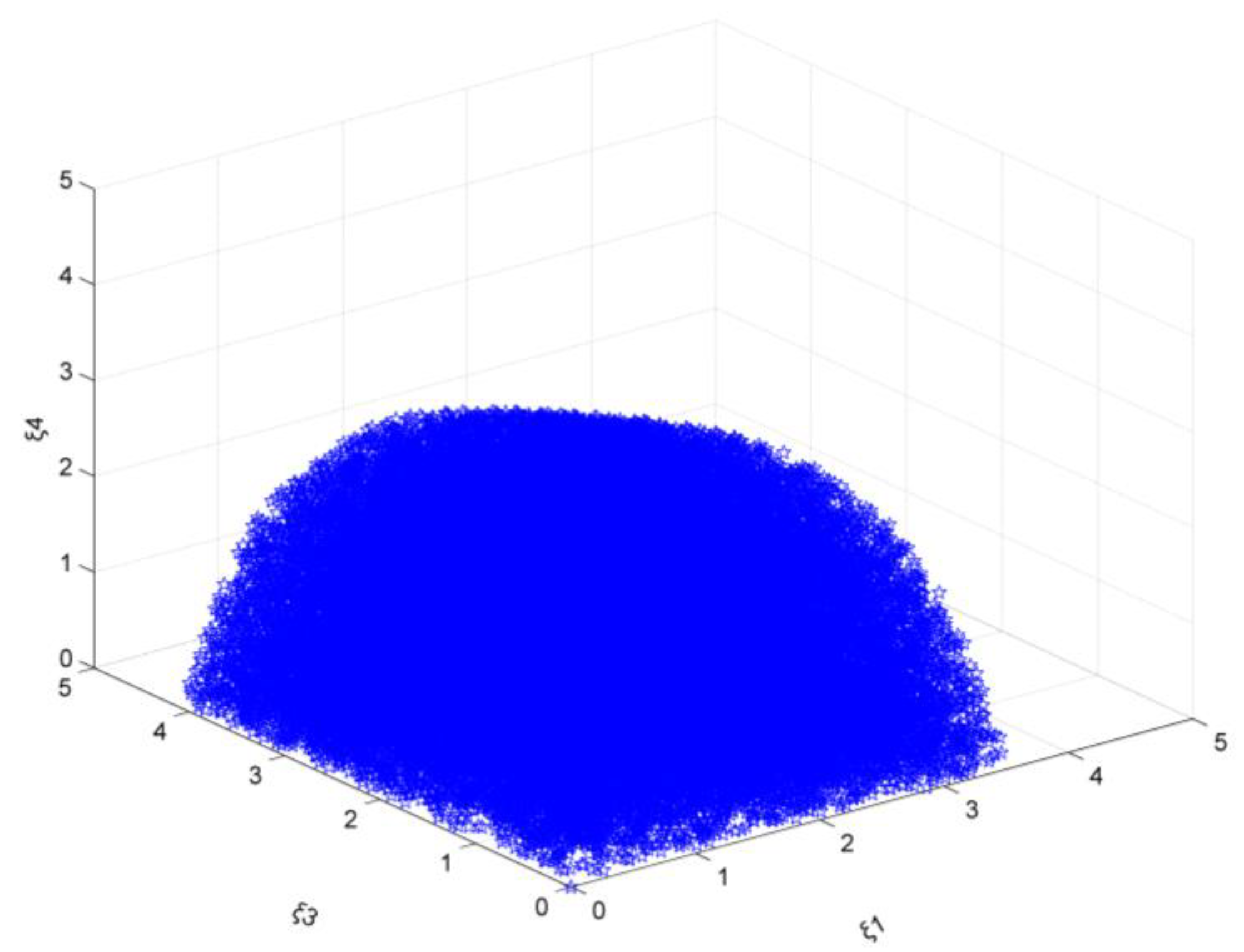
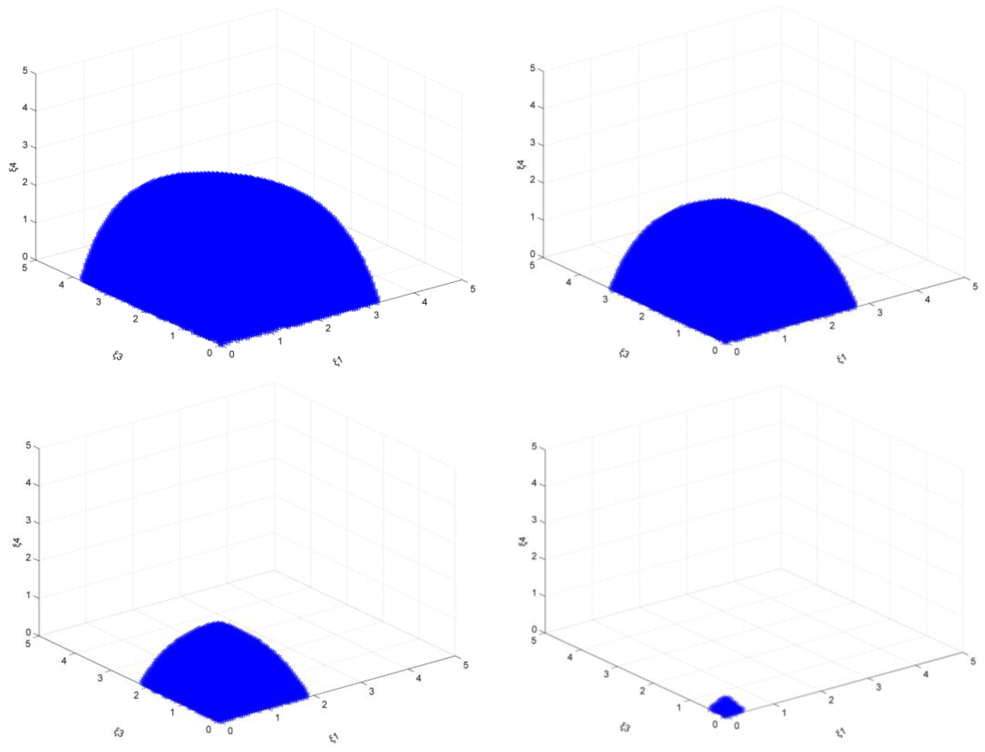
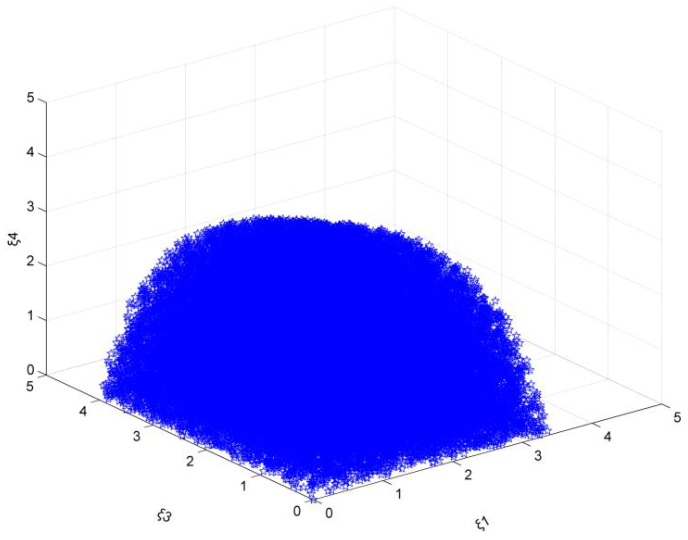
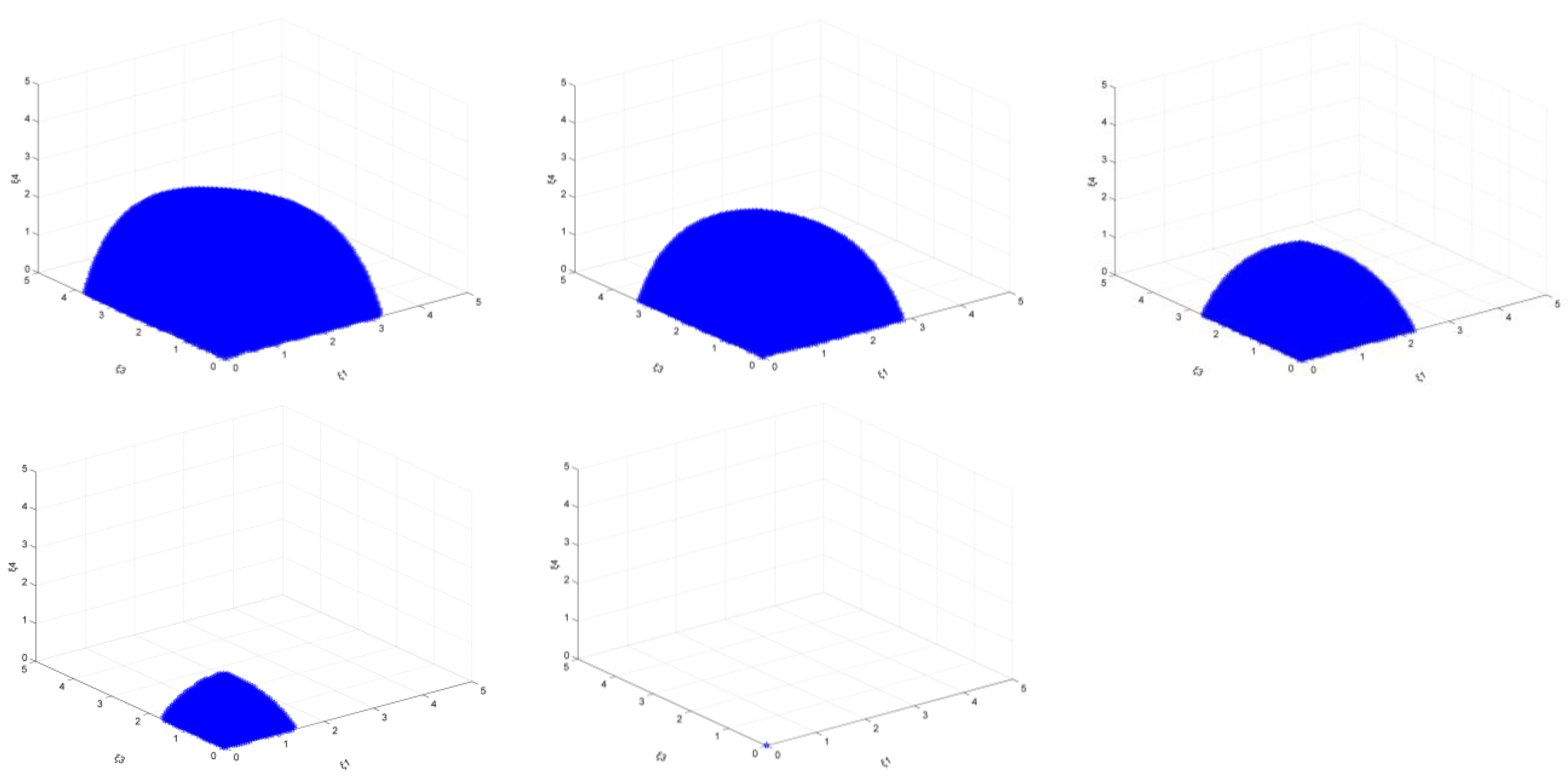
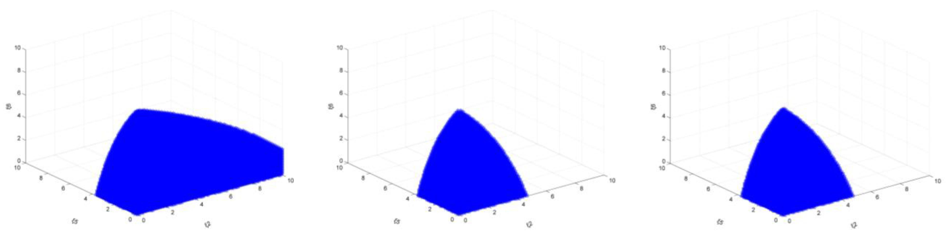
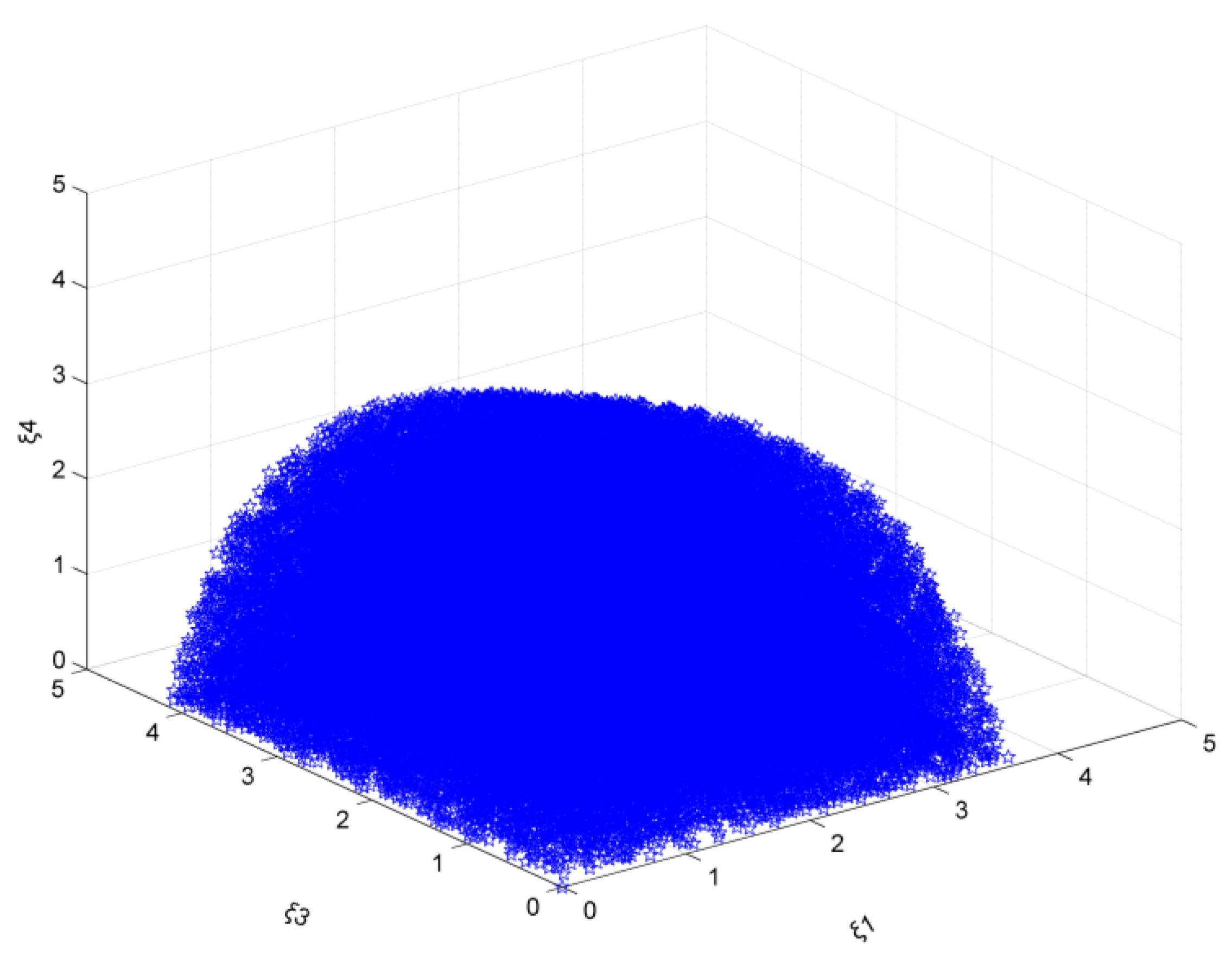
Figure 1.
The market stability domain (, emission reduction target: 16%).
Figure 1.
The market stability domain (, emission reduction target: 16%).
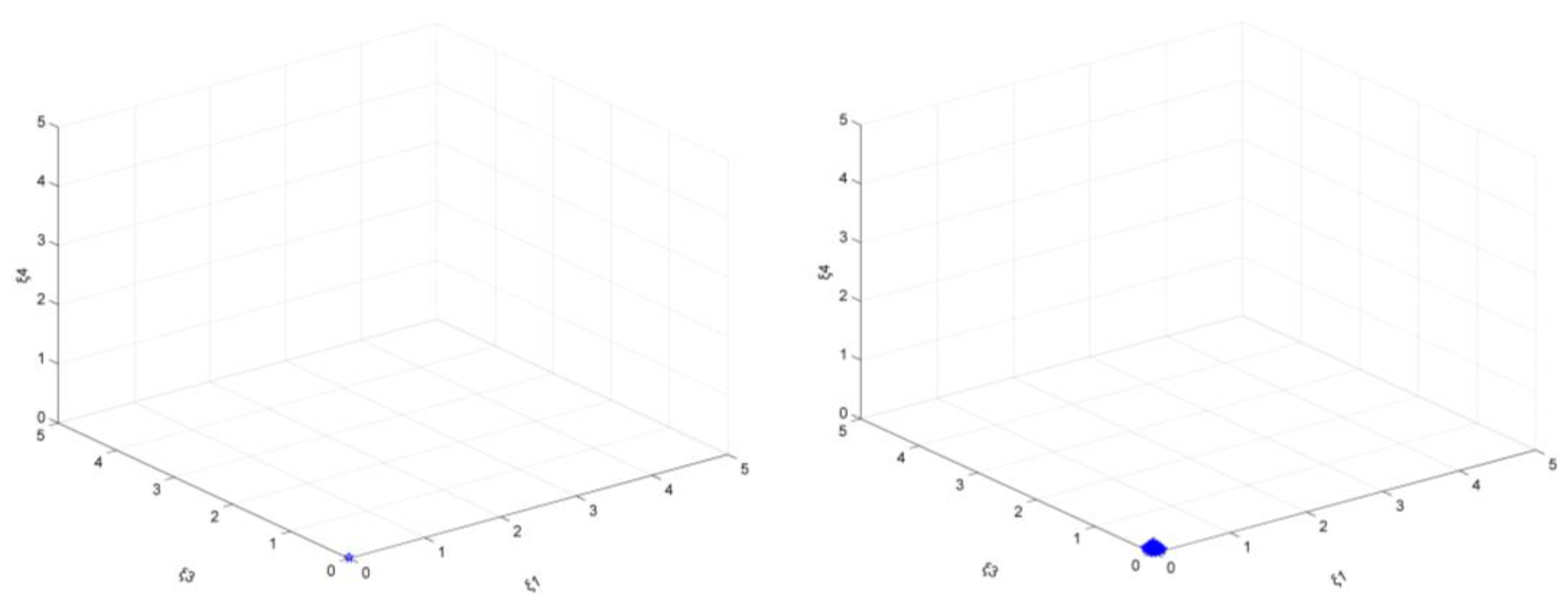
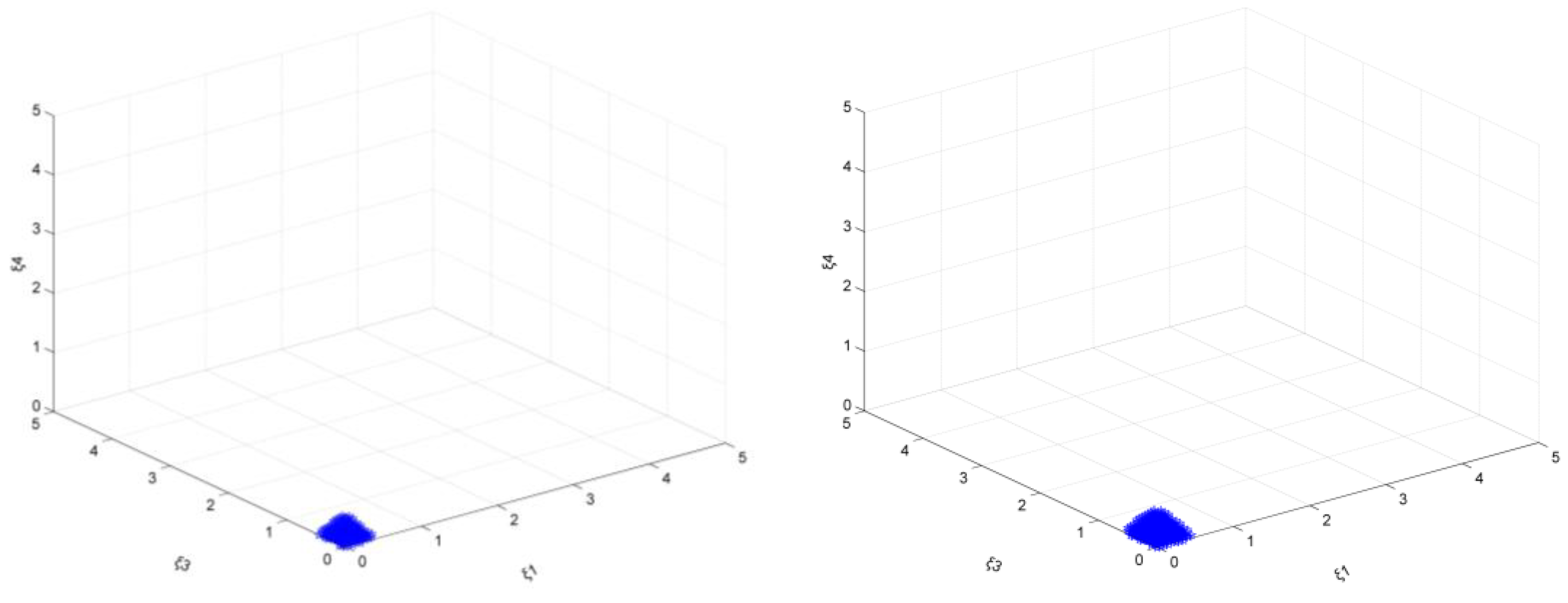
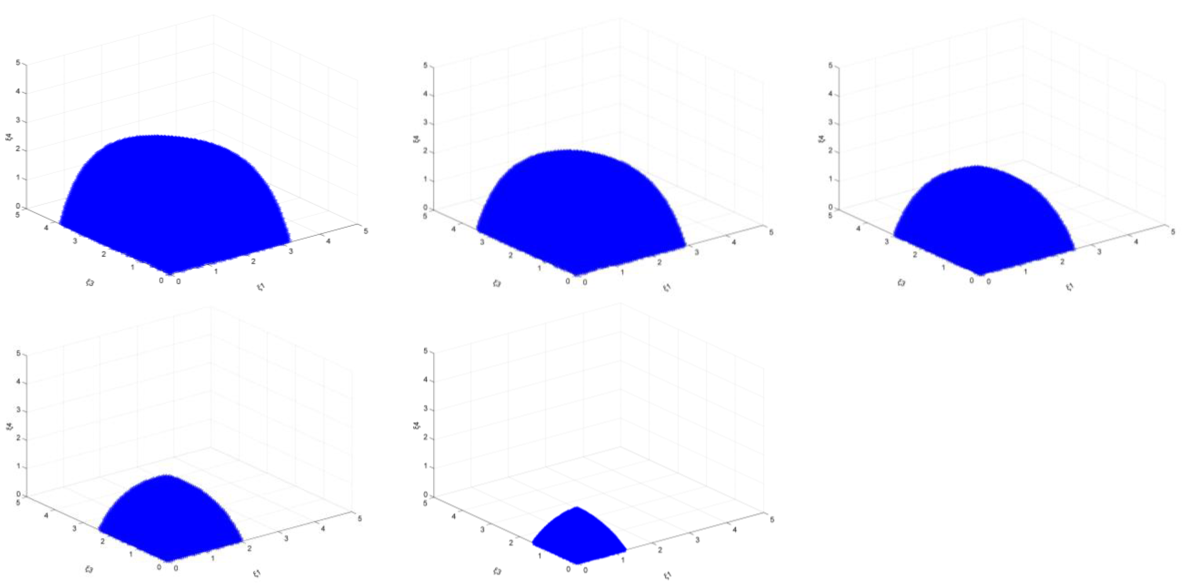
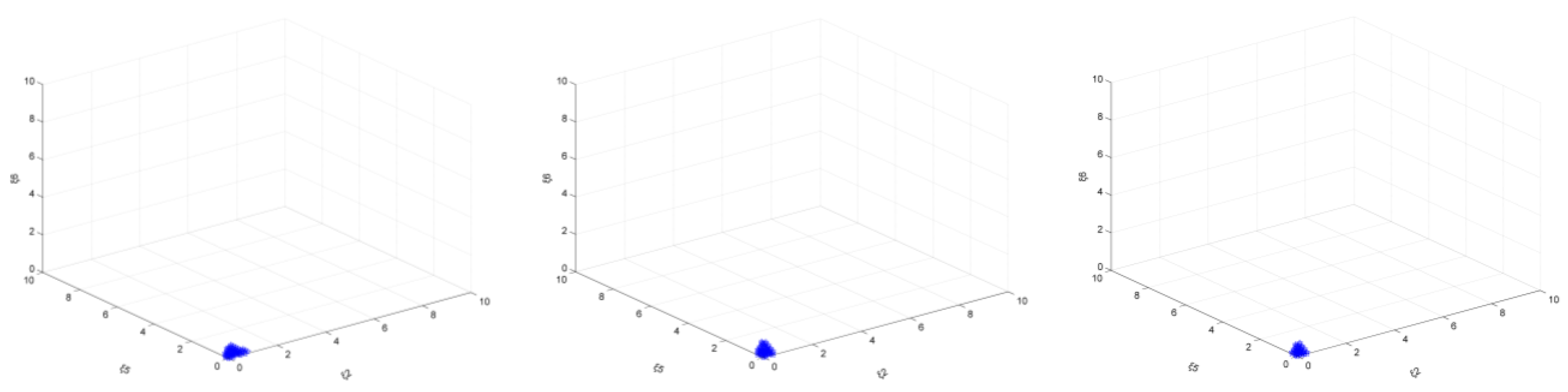
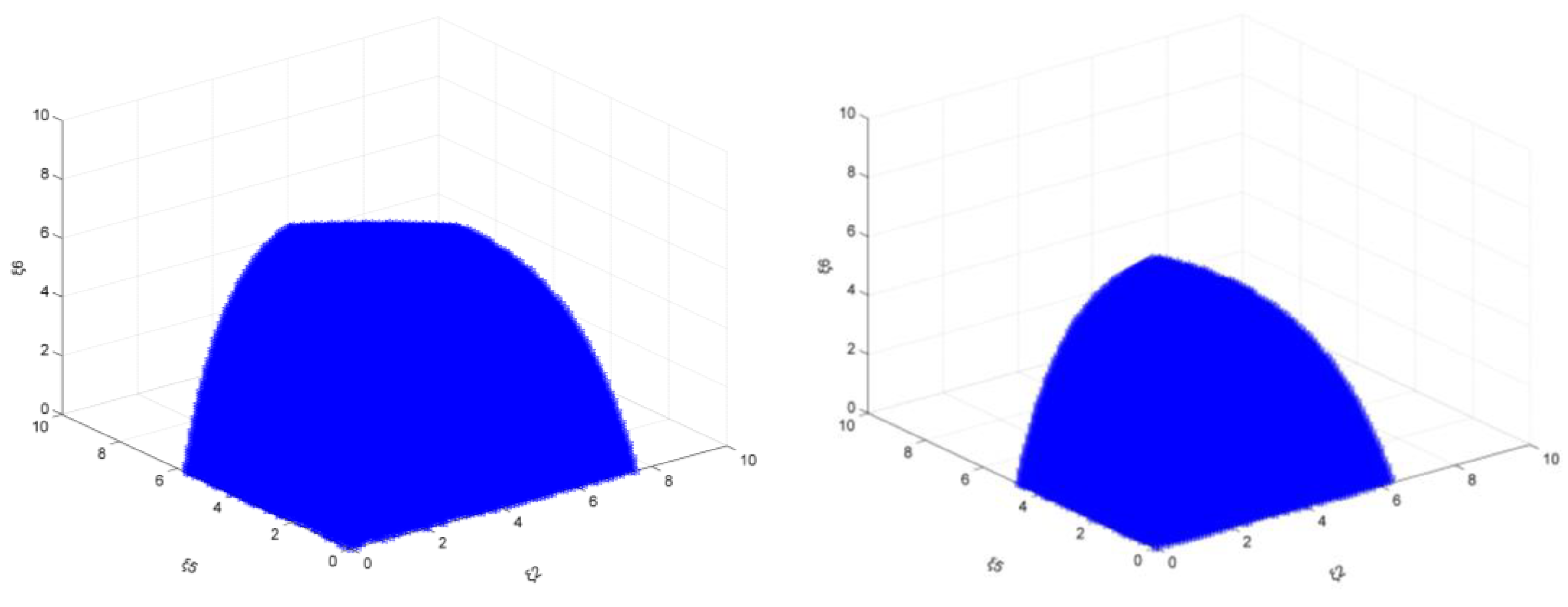
Figure 2.
The market stability domain (, emission reduction target: 16%).
Figure 2.
The market stability domain (, emission reduction target: 16%).
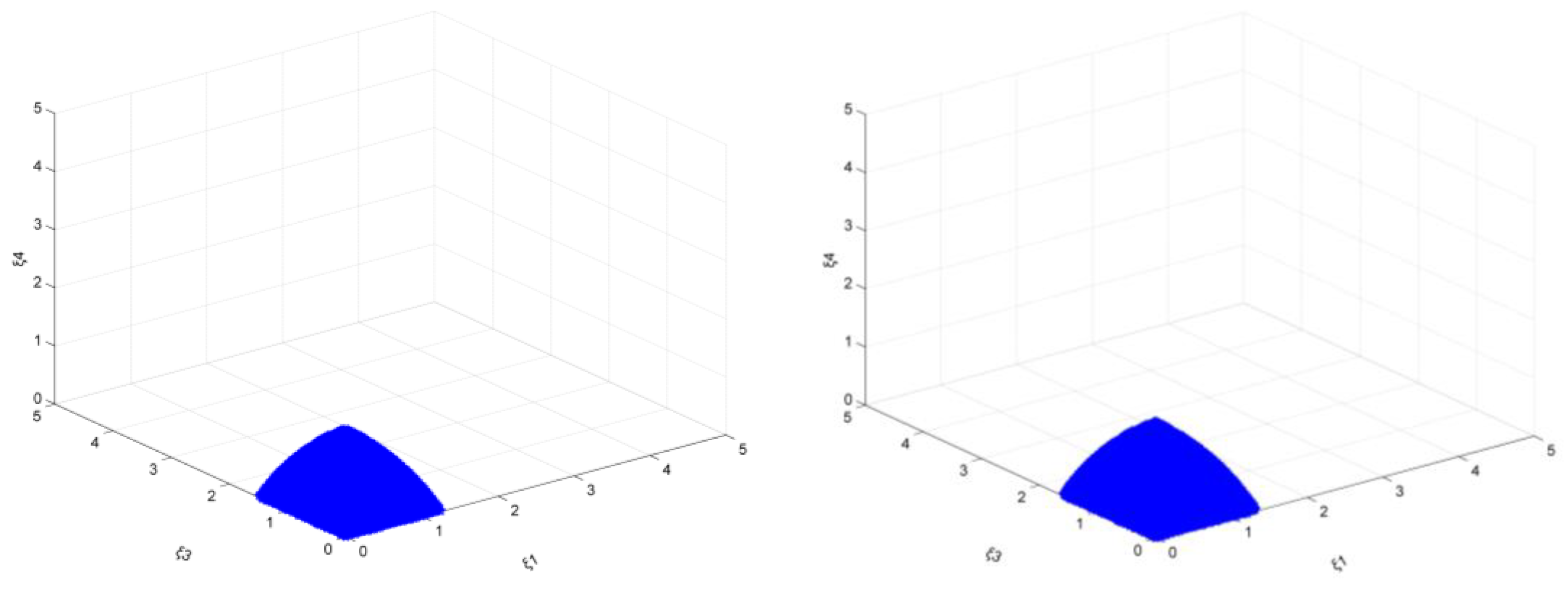
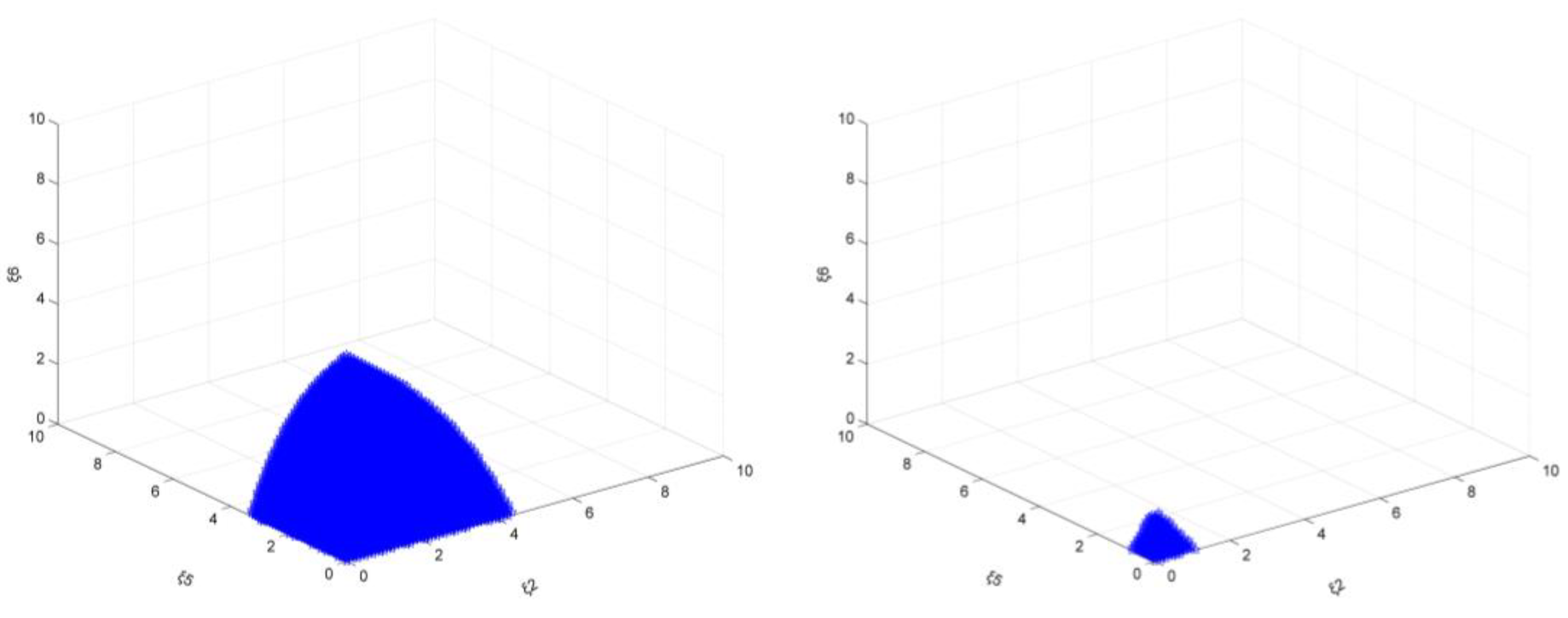
Figure 3.
The market stability domain (, emission reduction target: left 15%, right 20%).
Figure 3.
The market stability domain (, emission reduction target: left 15%, right 20%).
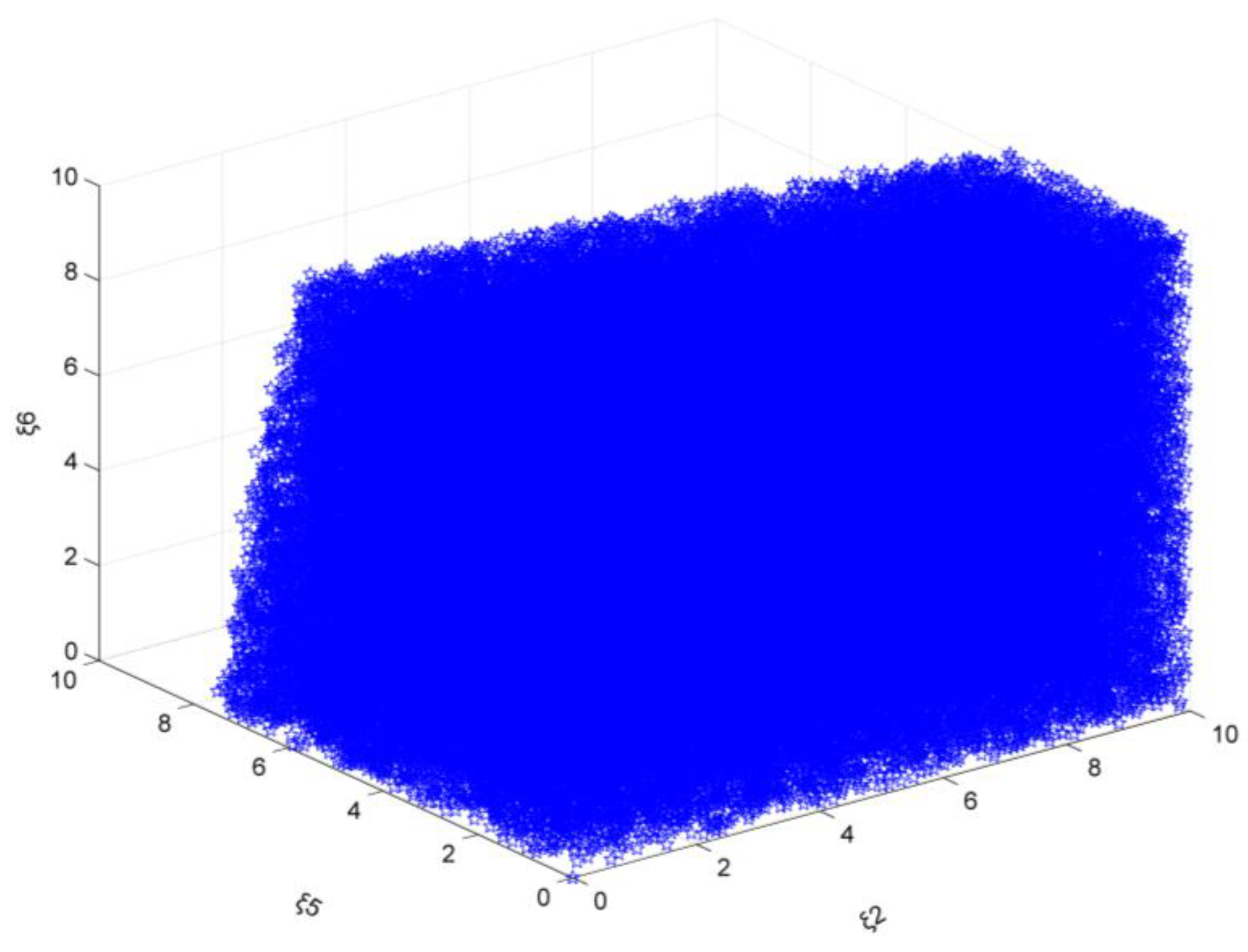
Figure 4.
The market stability domain (, emission reduction target: 16%).
Figure 4.
The market stability domain (, emission reduction target: 16%).
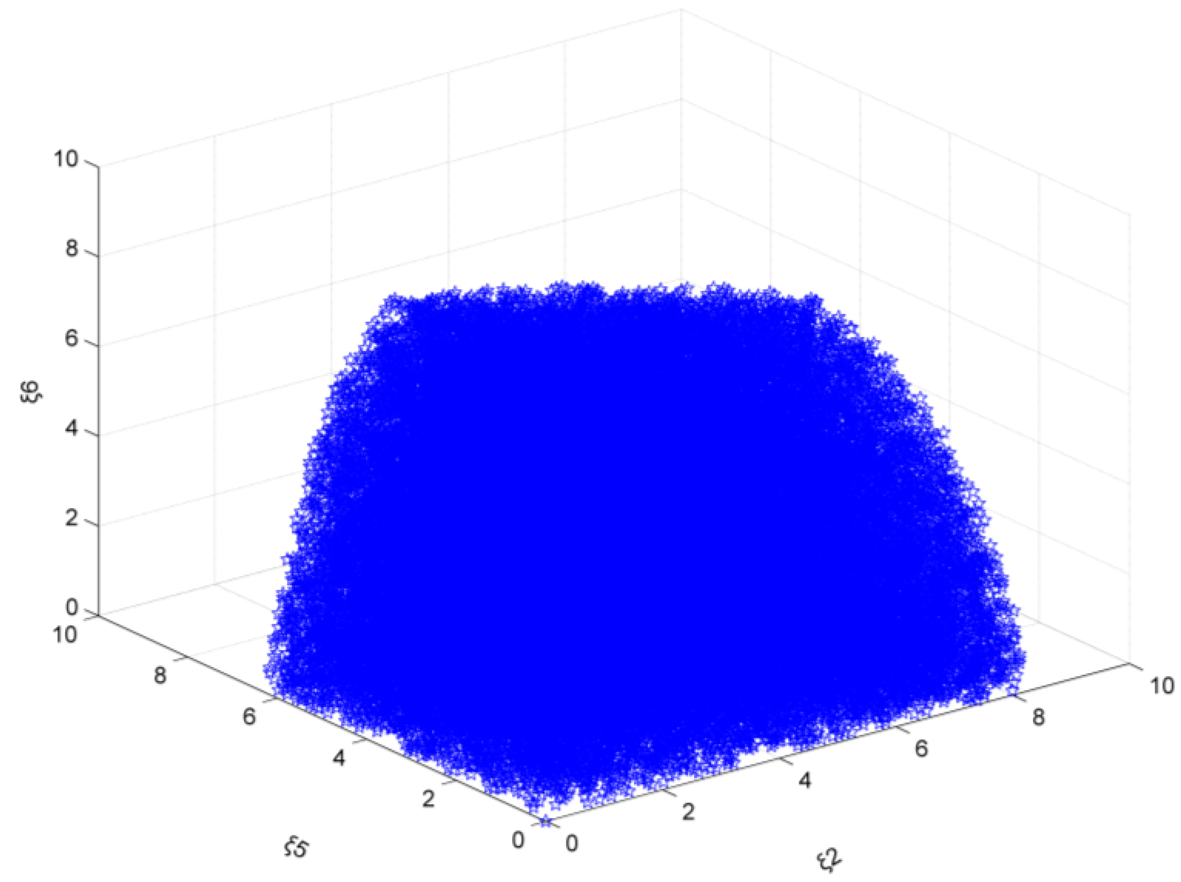
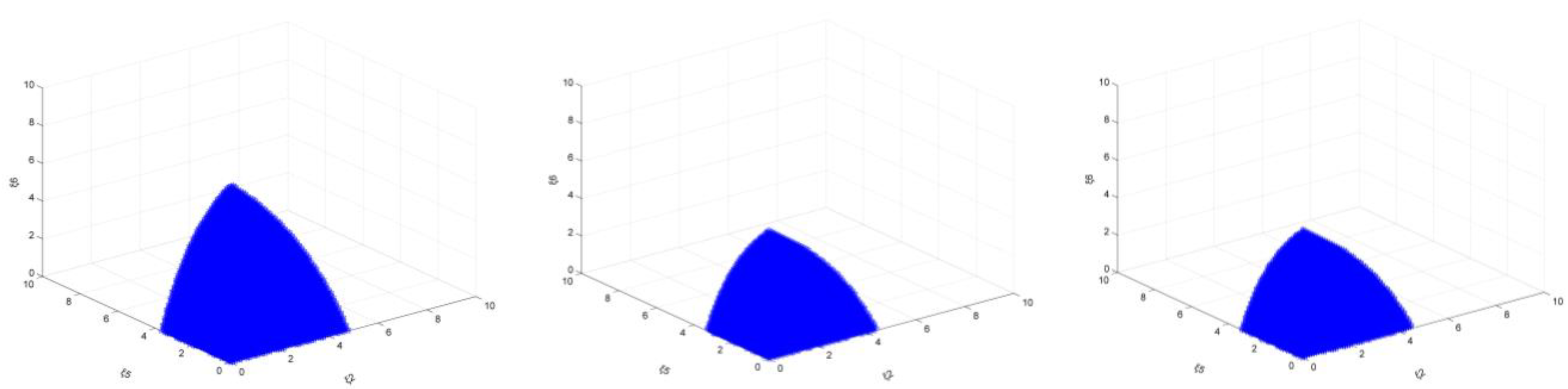
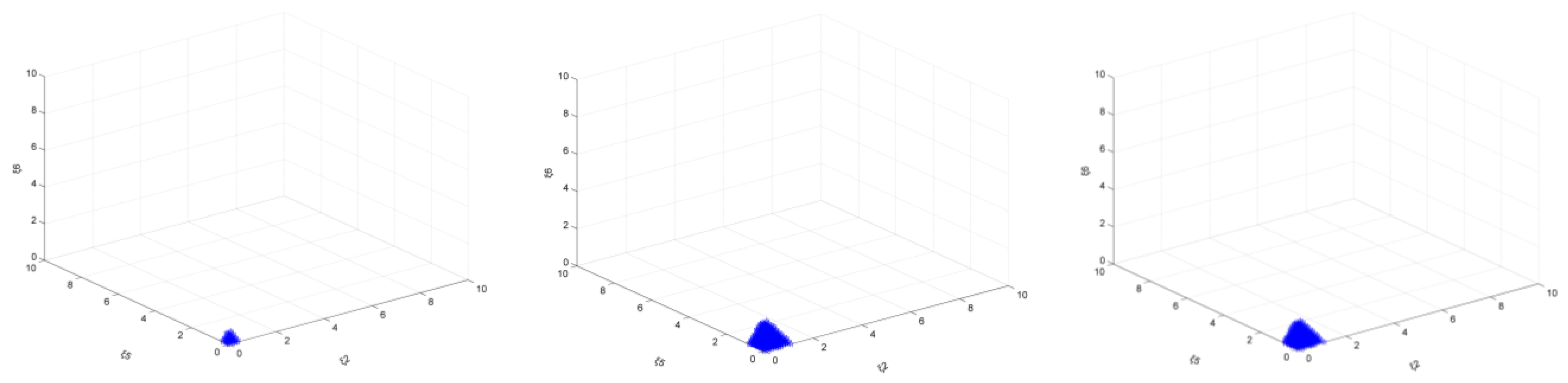
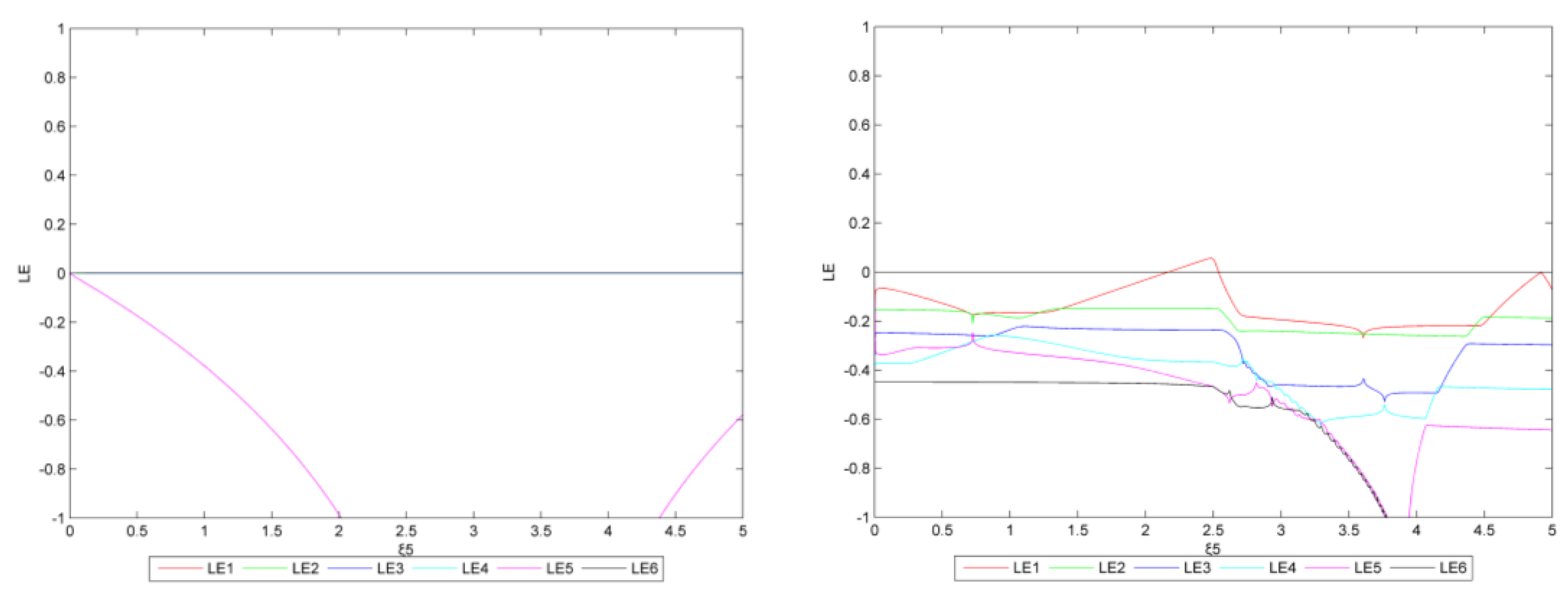
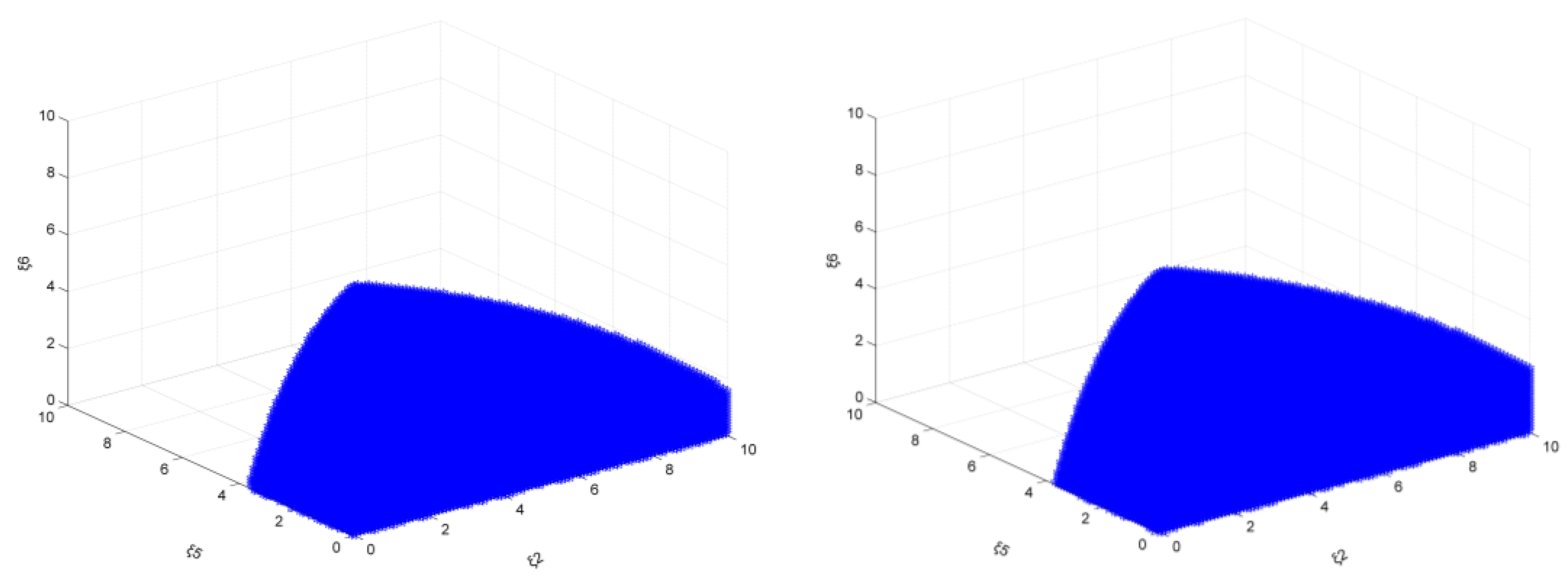
Figure 5.
Stability domain of the market (, emission reduction target: 16%).
Figure 5.
Stability domain of the market (, emission reduction target: 16%).
Figure 6.
The market stability domain (, emission reduction target: left 15%, right 20%).
Figure 6.
The market stability domain (, emission reduction target: left 15%, right 20%).
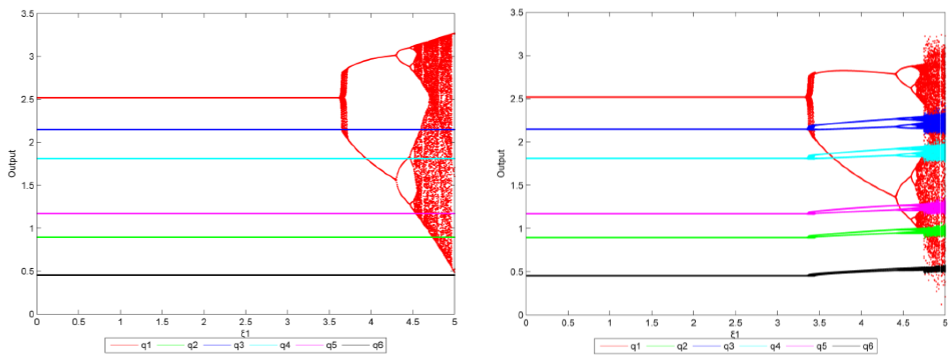
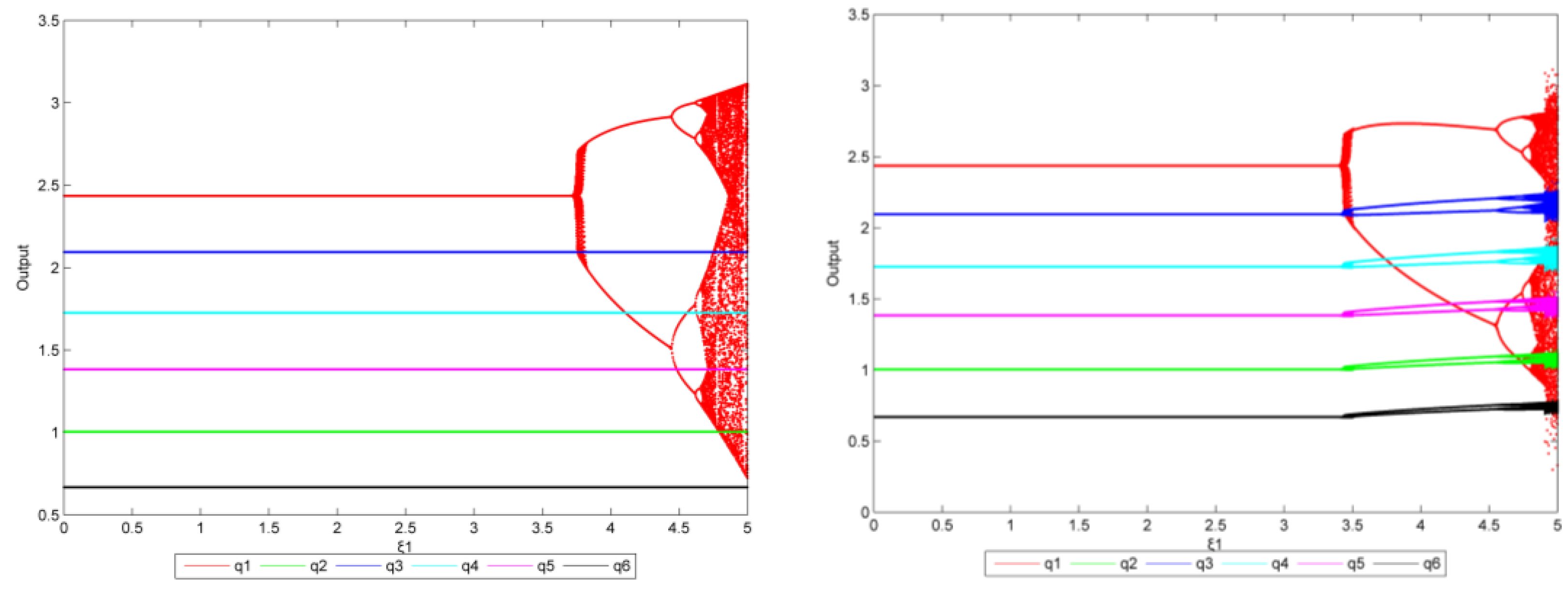
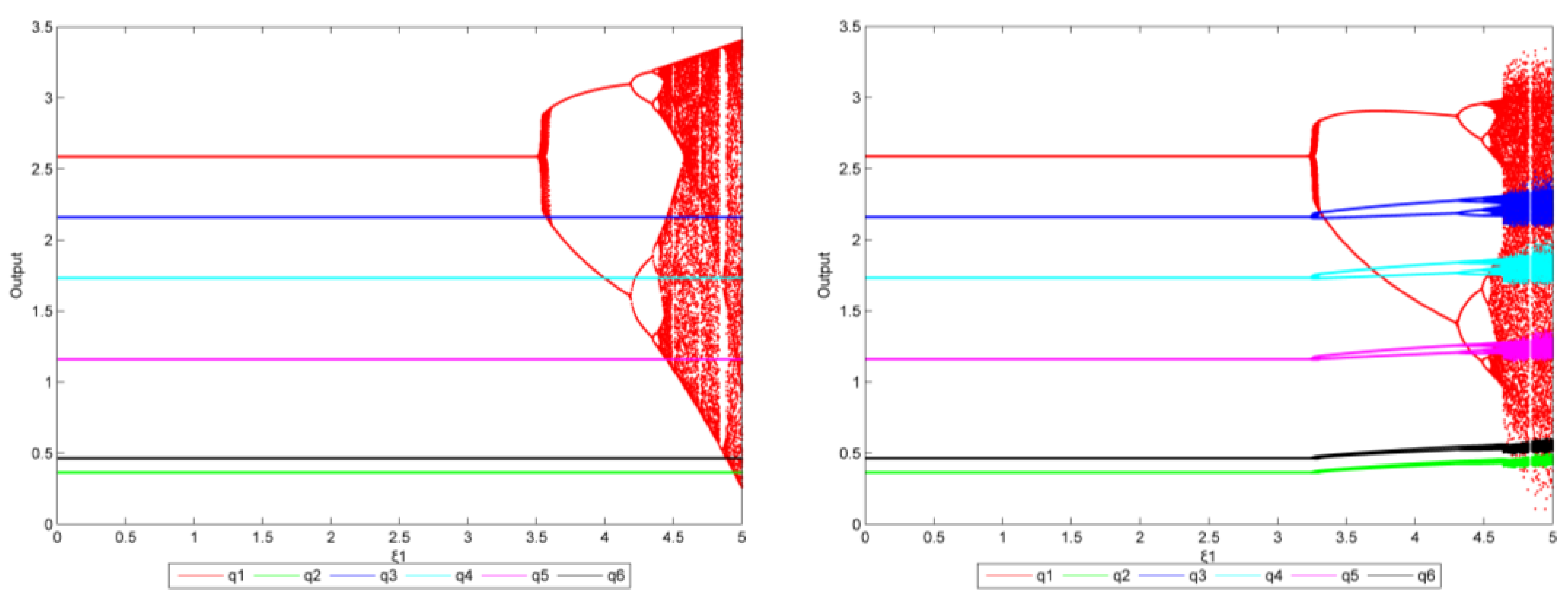
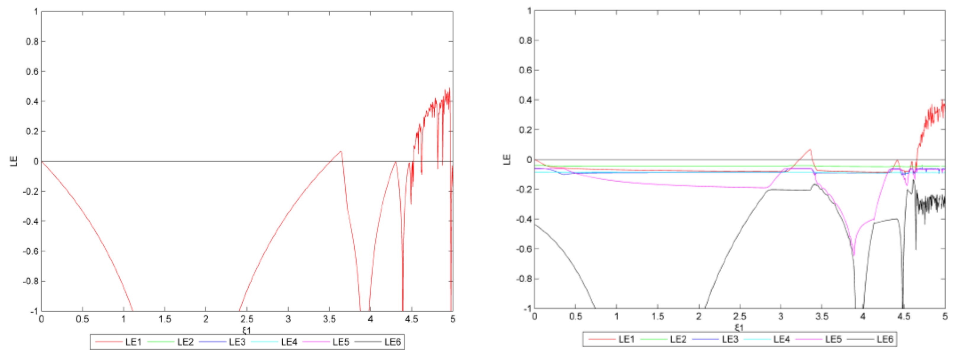
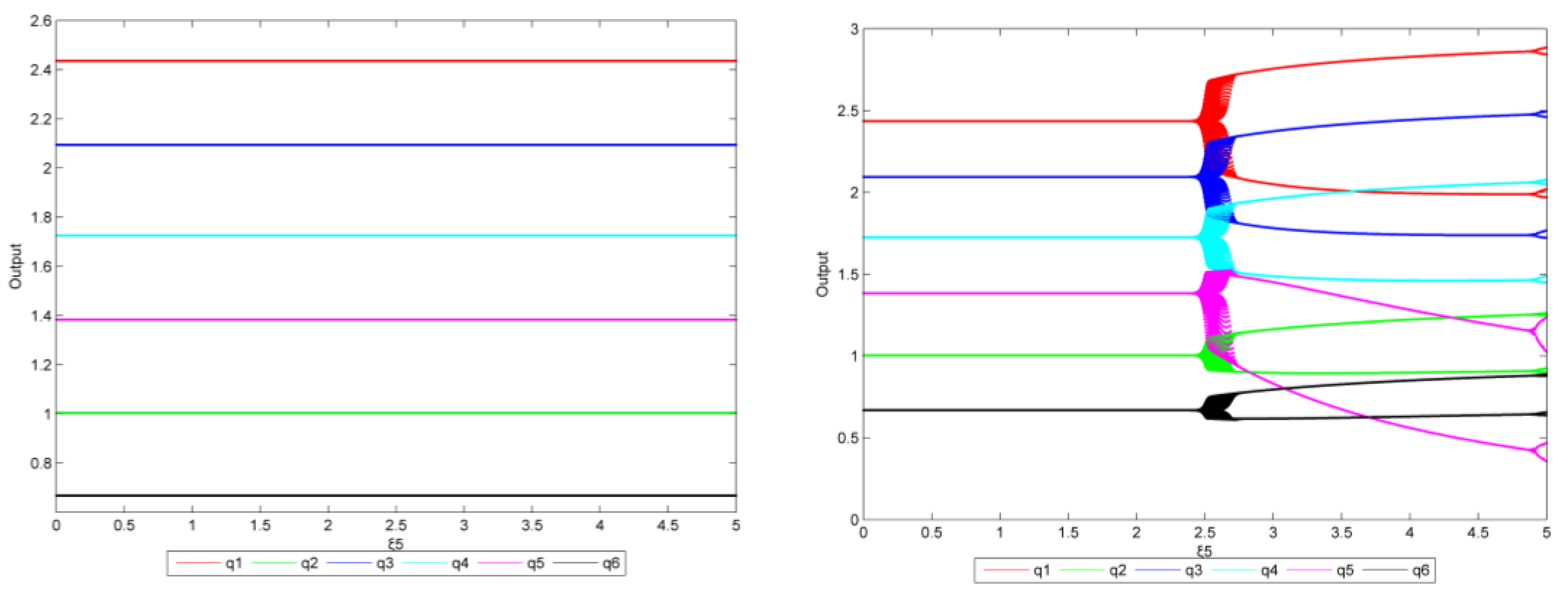
Figure 7.
The bifurcation diagram of (left: = 0, right: = 0.4, the reduction target is 20%).
Figure 7.
The bifurcation diagram of (left: = 0, right: = 0.4, the reduction target is 20%).
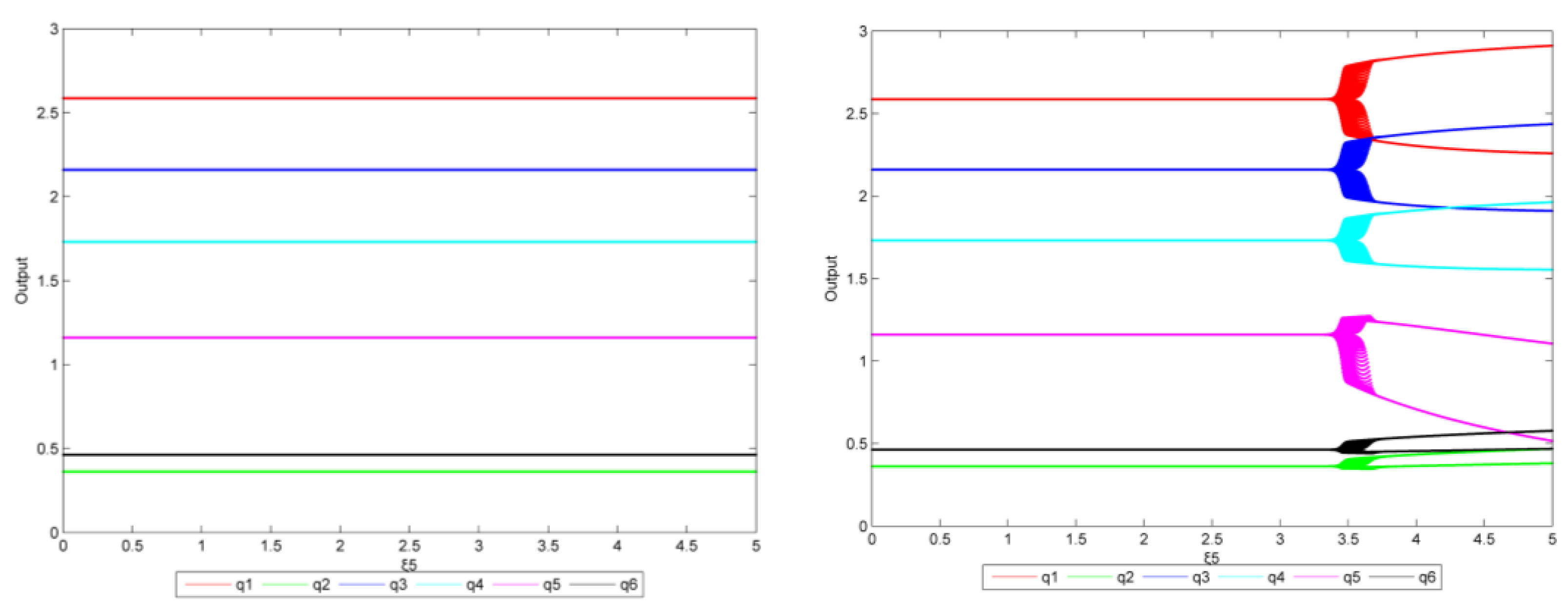
Figure 8.
The bifurcation diagram of (left: = 0, right: = 1.5, the reduction target is 20%).
Figure 8.
The bifurcation diagram of (left: = 0, right: = 1.5, the reduction target is 20%).
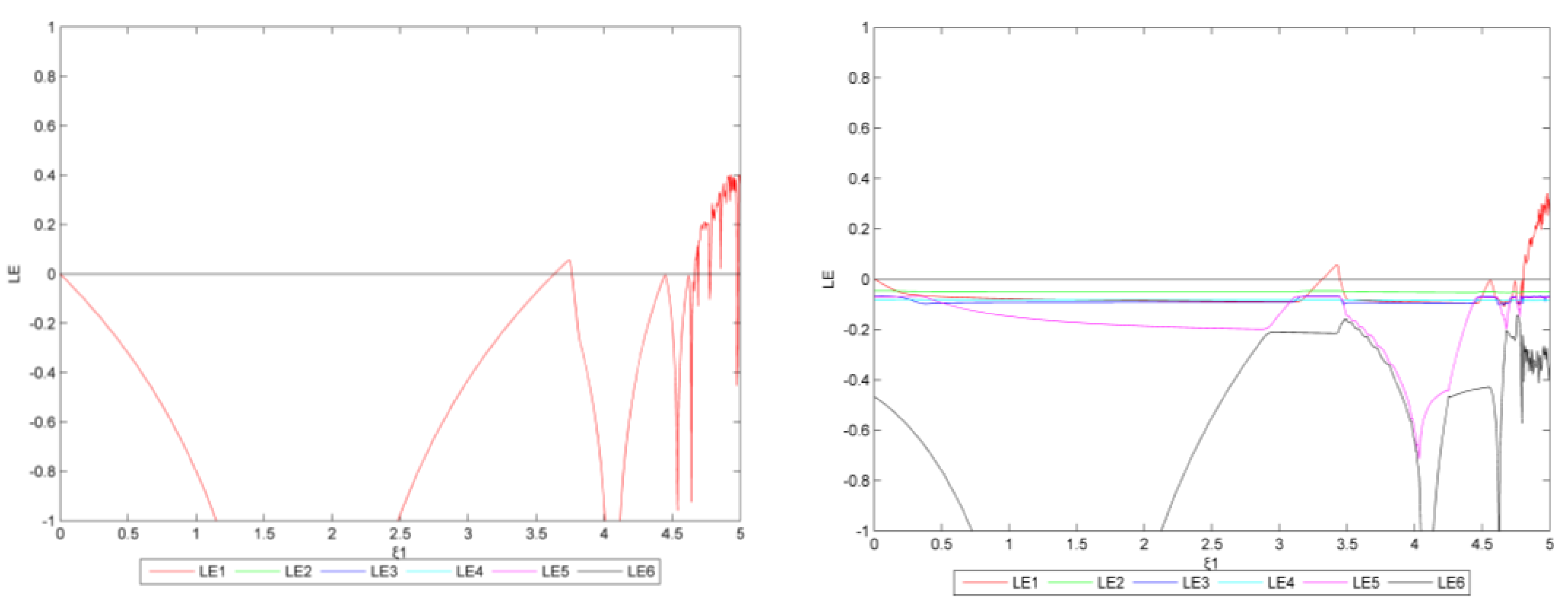
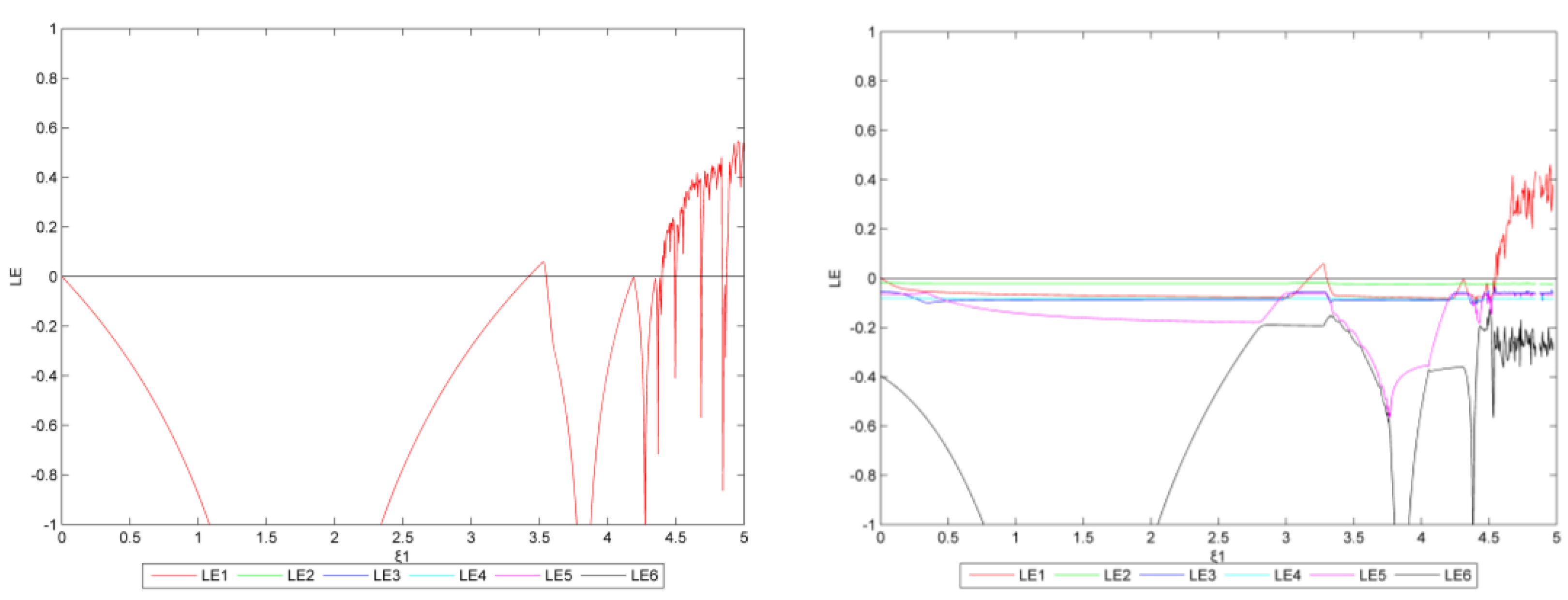
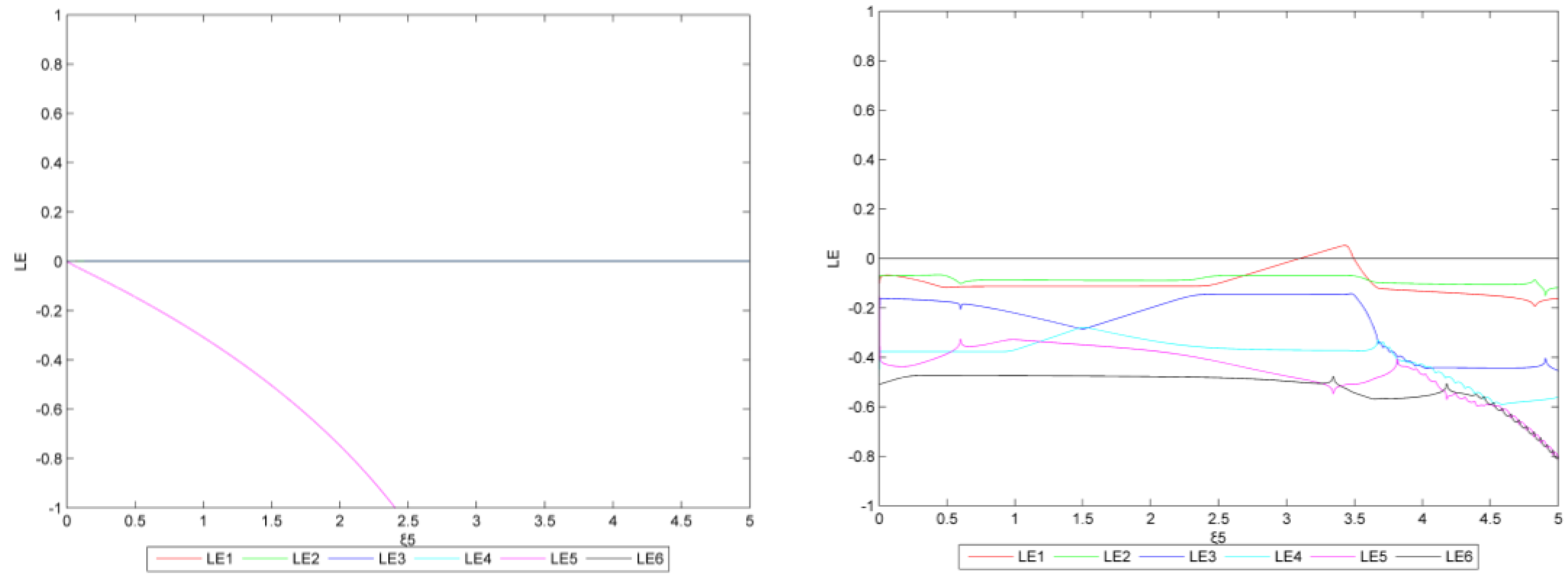
Figure 9.
The Lyapunov exponent diagram (left: = 0, right: = 0.4, the reduction target is 20%).
Figure 9.
The Lyapunov exponent diagram (left: = 0, right: = 0.4, the reduction target is 20%).
Figure 10.
The Lyapunov exponent diagram (left: = 0, right: = 1.5, the reduction target is 20%).
Figure 10.
The Lyapunov exponent diagram (left: = 0, right: = 1.5, the reduction target is 20%).
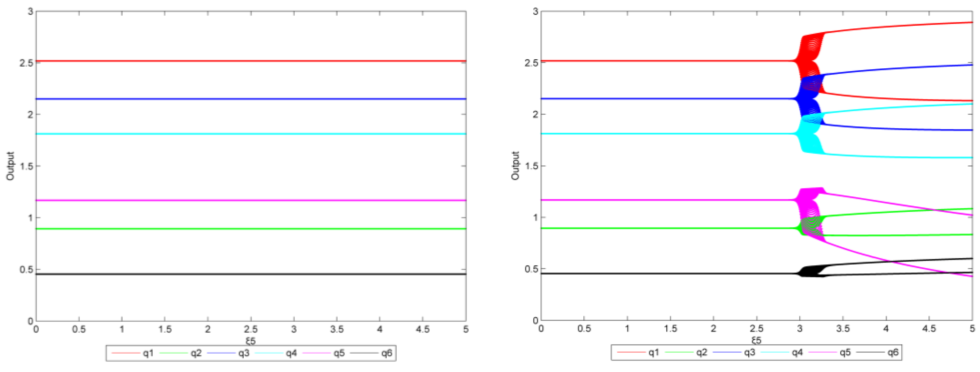
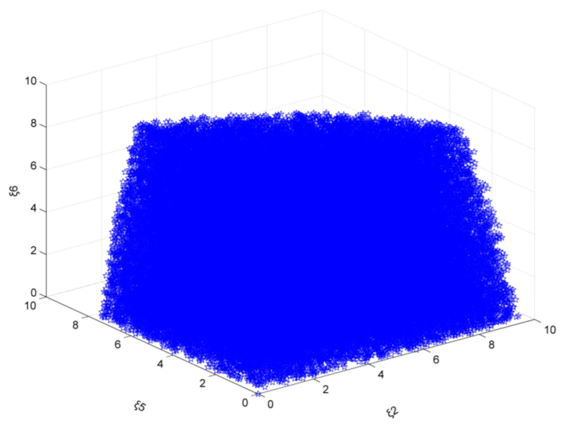
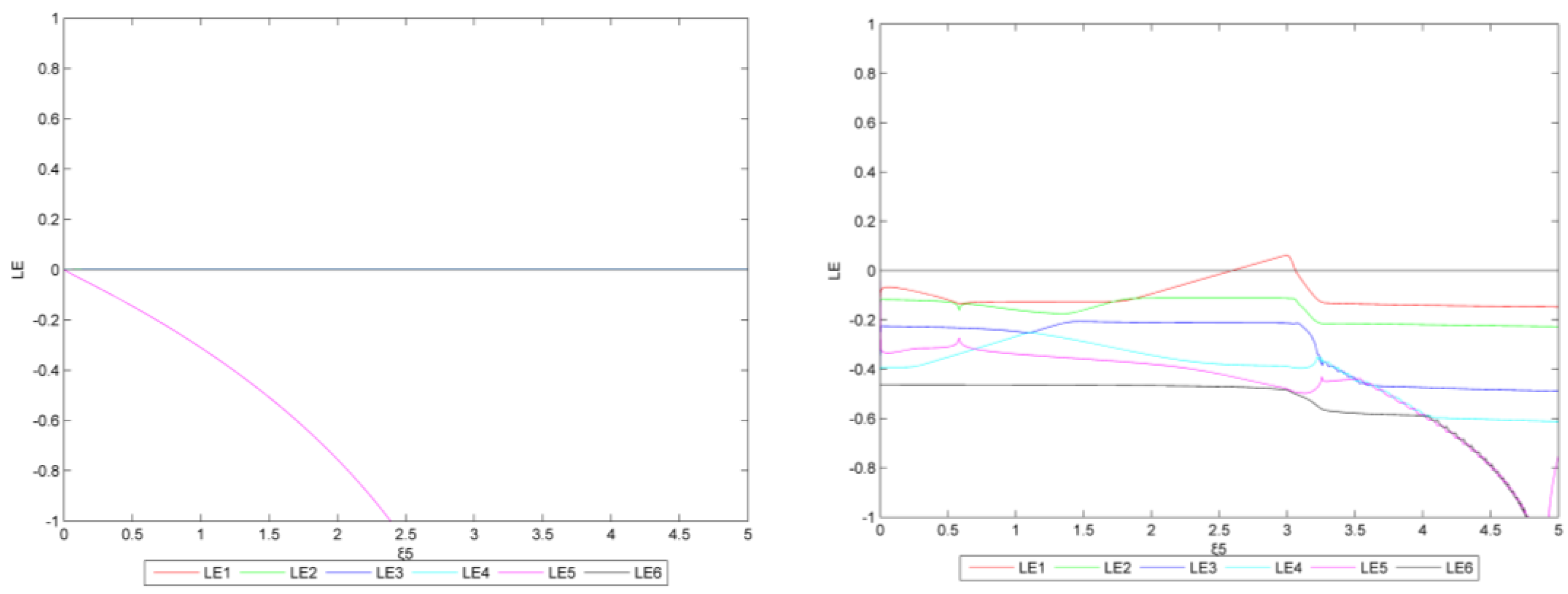
Figure 11.
The market stability (, emission reduction target: 20%).
Figure 11.
The market stability (, emission reduction target: 20%).
Figure 12.
The market stability domain (, emission reduction target: 20%).
Figure 12.
The market stability domain (, emission reduction target: 20%).
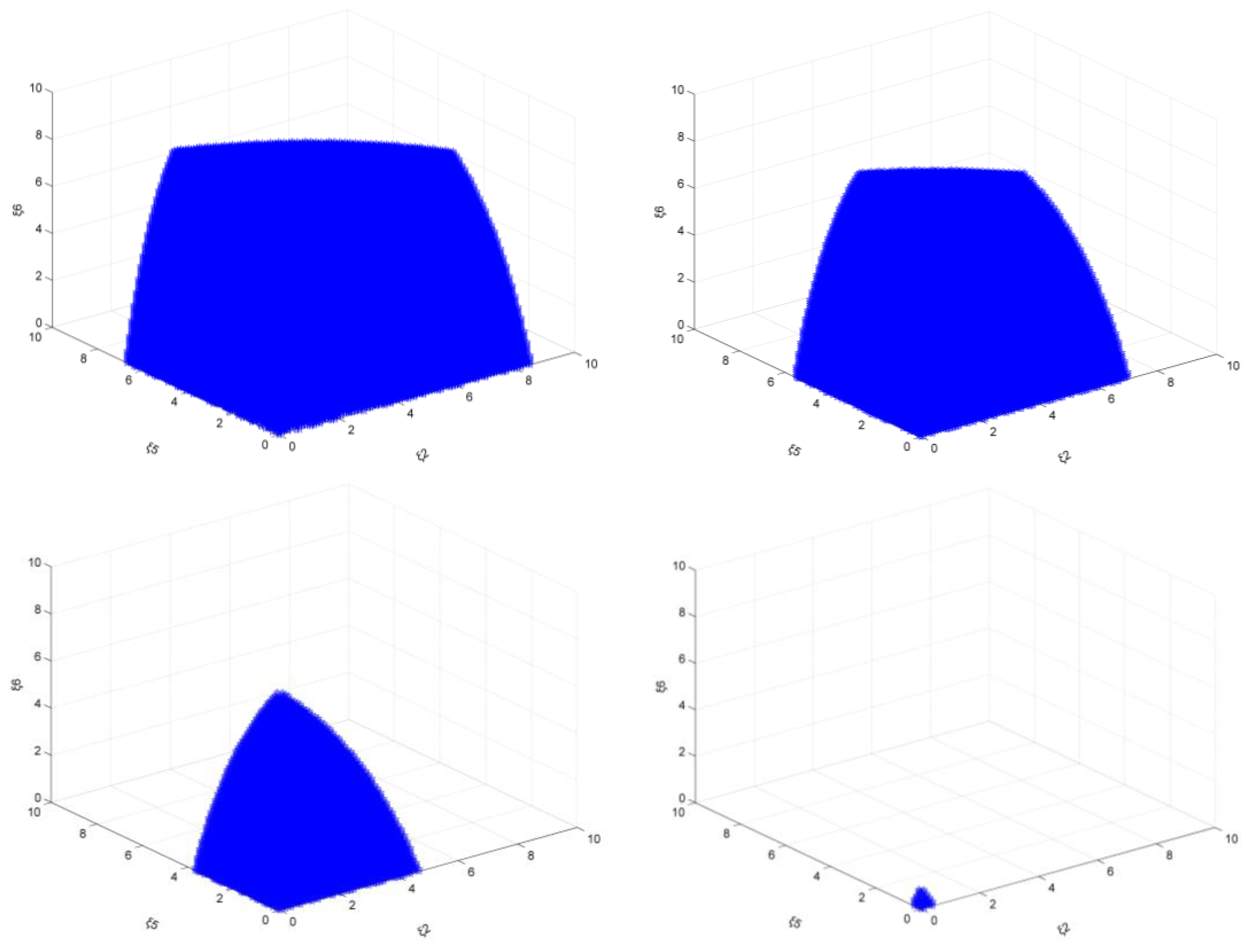
Figure 13.
The market stability domain (, emission reduction target: left 20%, right 25%).
Figure 13.
The market stability domain (, emission reduction target: left 20%, right 25%).
Figure 14.
The market stability domain (, emission reduction target: 20%).
Figure 14.
The market stability domain (, emission reduction target: 20%).
Figure 15.
The market stability domain (, emission reduction target: 20%).
Figure 15.
The market stability domain (, emission reduction target: 20%).
Figure 16.
The market stability domain (, emission reduction target: left 20% (2020), middle 20% (2025), right 25%).
Figure 16.
The market stability domain (, emission reduction target: left 20% (2020), middle 20% (2025), right 25%).
Figure 17.
The market stability domain (, emission reduction target: left 20% (2020), middle 20% (2025), right 25%).
Figure 17.
The market stability domain (, emission reduction target: left 20% (2020), middle 20% (2025), right 25%).
Figure 18.
The bifurcation diagram of (left: = 0, right: = 0.4, the reduction target is 25%).
Figure 18.
The bifurcation diagram of (left: = 0, right: = 0.4, the reduction target is 25%).
Figure 19.
The bifurcation diagram of (left: = 0, right: = 1.5, the reduction target is 25%).
Figure 19.
The bifurcation diagram of (left: = 0, right: = 1.5, the reduction target is 25%).
Figure 20.
The Lyapunov exponent diagram (left: = 0, right: = 0.4, the reduction target is 25%).
Figure 20.
The Lyapunov exponent diagram (left: = 0, right: = 0.4, the reduction target is 25%).
Figure 21.
The Lyapunov exponent diagram (left: = 0, right: = 1.5, the reduction target is 25%).
Figure 21.
The Lyapunov exponent diagram (left: = 0, right: = 1.5, the reduction target is 25%).
Figure 22.
The market stability domain (, emission reduction target: 25%).
Figure 22.
The market stability domain (, emission reduction target: 25%).
Figure 23.
The market stability domain (, emission reduction target: 25%).
Figure 23.
The market stability domain (, emission reduction target: 25%).
Figure 24.
The market stability domain (, emission reduction target: left 25%, right 30%).
Figure 24.
The market stability domain (, emission reduction target: left 25%, right 30%).
Figure 25.
The market stability domain (, emission reduction target: 25%).
Figure 25.
The market stability domain (, emission reduction target: 25%).
Figure 26.
The market stability domain (, emission reduction target: 25%).
Figure 26.
The market stability domain (, emission reduction target: 25%).
Figure 27.
The market stability domain (, emission reduction target: left 25% (2025), middle 25% (2030), right 30%).
Figure 27.
The market stability domain (, emission reduction target: left 25% (2025), middle 25% (2030), right 30%).
Figure 28.
The market stability domain (, emission reduction target: left 25% (2025), middle 25% (2030), right 30%).
Figure 28.
The market stability domain (, emission reduction target: left 25% (2025), middle 25% (2030), right 30%).
Figure 29.
The bifurcation diagram of (left: = 0, right: = 0.4, the reduction target is 30%).
Figure 29.
The bifurcation diagram of (left: = 0, right: = 0.4, the reduction target is 30%).
Figure 30.
The bifurcation diagram of (left: = 0, right: = 1.5, the reduction target is 30%).
Figure 30.
The bifurcation diagram of (left: = 0, right: = 1.5, the reduction target is 30%).
Figure 31.
The Lyapunov exponent diagram (left: = 0, right: = 0.4, the reduction target is 30%).
Figure 31.
The Lyapunov exponent diagram (left: = 0, right: = 0.4, the reduction target is 30%).
Figure 32.
The Lyapunov exponent diagram (left: = 0, right: = 1.5, the reduction target is 30%).
Figure 32.
The Lyapunov exponent diagram (left: = 0, right: = 1.5, the reduction target is 30%).
Table 1.
The literature and summary information on carbon tax applied to the steel industry.
Table 1.
The literature and summary information on carbon tax applied to the steel industry.
| Researcher | Main Theory and Model |
|---|
| Mathiesen and Maestad [9] | partial equilibrium model |
| Liang et al. [10] | CGE model |
| Nie et al. [11] | C-D production function |
| Kuo et al. [12] | evolutionary game |
| Wakiyama and Zusman [13] | time-series autoregressive moving average (ARMA) model |
| Duan et al. [14,15] | dynamic game |
| Ntombela et al. [16] | CGE model |
| Li et al. [17] | environmental-economic simulation model |
| Zhu et al. [18] | CGE model |
| Wu and Xie [19] | CGE model and the optimization model |
| Deng and Adams [20] | life cycle assessment |
| Liu et al. [21] | life cycle assessment |
| Zhao et al. [22] | supply chain analysis |
Table 2.
The literature about bounded rationality in industry application.
Table 2.
The literature about bounded rationality in industry application.
| Researcher | Industrial Sector |
|---|
| Ji [23] | electricity industry and electricity market |
| Sun and Ma [24] | steel industry and steel market |
| Tu [25] | power and renewable resources industry |
| Dang and Hong [26] | glass substrates industry |
| Tan and Liang [27] | coal industry and coal market |
| Li et al. [28] | tourism industry |
| Di et al. [29,30] | transportation planning |
| Liu [31] | carbon trade market |
| Yu [32] | transportation industry |
| Ding et al. [33] | electricity system |
| Zhang [34] | carbon trade market |
| Sang, Xie and Wang [35] | ship-building industry |
| Zhang et al. [36] | remanufacturing industry |
| Wu [37] | electricity market |
| Duan et al. [38] | steel industry |
| Rezvani and Hudson [39] | oil and gas industry |
| Fan et al. [40] | coal Industry |
| Gao et al. [41] | creative industry |
| Ma et al. [42] | vehicle industry |
| Hammond et al. [43] | construction industry |
Table 3.
Notations and explanations used in this paper.
Table 3.
Notations and explanations used in this paper.
| Notations | Explanations |
|---|
| Q | Steel production |
| P | The price of steel |
| α | The constant of the market inverse demand curve |
| β | The primary coefficient of the market inverse demand curve |
| qi | Steel production of region i |
| e2015,i | The region i CO2 emission intensity of per ton steel in 2015 |
| ei | The region i CO2 emission intensity of per ton steel at some stage |
| ri | The decline range of CO2 emission intensity of per ton steel in region i at some stage |
| R | The decline target of national CO2 emission intensity of per ton steel at some stage |
| MAC | Marginal abatement cost curve in steel industry |
| ai | The quadratic coefficient of steel industry’s MAC in region i |
| bi | The primary coefficient of steel industry’s MAC in region i |
| Ci | The cost function of steel industry in region i |
| C0,i | The production cost of steel industry in region i |
| ci | The cost of base period emission reduction in region i |
| T | The total carbon tax |
| t | The unit value of carbon tax |
| W | Social welfare function |
| CS | Consumer surplus |
| PS | Producer surplus |
| D(E) | Total macro external environment loss of CO2 emission |
| θ | The external loss parameter of CO2 |
| πi | The profit function of steel industry in region i |
| E | The total CO2 emissions in steel industry |
| ξi | The adjustment coefficient, rate of output adjustment |
| η | The production subsidies |
| m | The CO2 emission reduced by the CCS demonstration project |
| A | The primary coefficient of CCS demonstration project cost curve |
| B | The constant of the CCS demonstration project cost curve |
| S | The total subsidy |
| M | The total cost of the CCS demonstration project |
Table 4.
Some major parameter values in this research.
Table 4.
Some major parameter values in this research.
| Notations | Unit | i = 1 | i = 2 | i= 3 | i = 4 | i = 5 | i = 6 |
|---|
| e2015,i | t CO2/t | 2.3344 | 3.5698 | 2.9040 | 2.8779 | 3.2202 | 4.5864 |
| ai | - | 11,661 | 17,208 | 16,932 | 12,952 | 6397.2 | 3485 |
| bi | - | −169.76 | 8876.7 | −166.92 | 1483.6 | 502.52 | 421.13 |
| ci | Yuan | 2168.2 | 3511.1 | 2165.4 | 3325.1 | 2368.7 | 3814.3 |
| C0,case,k,i | Yuan, 2015 | 2833.15 | 4898.47 | 3453.53 | 4153.15 | 3799.03 | 3832.38 |
| Yuan, 2020 | 2124.86 | 3918.77 | 2590.15 | 2491.89 | 3609.08 | 3640.76 |
| Yuan, 2025 | 1699.89 | 2743.14 | 2072.12 | 1868.92 | 3067.72 | 3094.64 |
| Yuan, 2030 | 1444.91 | 2194.51 | 1761.30 | 1588.58 | 2454.17 | 2475.71 |
Table 5.
The equilibrium output E* of each regional enterprise (emission reduction target: 15–20%).
Table 5.
The equilibrium output E* of each regional enterprise (emission reduction target: 15–20%).
| Emission Reduction Target | 15% | 16% | 17% | 18% | 19% | 20% |
|---|
| q1 | 2.5789 | 2.5803 | 2.5817 | 2.5833 | 2.5850 | 2.5867 |
| q2 | 0.3823 | 0.3793 | 0.3758 | 0.3720 | 0.3677 | 0.3629 |
| q3 | 2.1623 | 2.1619 | 2.1614 | 2.1609 | 2.1603 | 2.1597 |
| q4 | 1.7354 | 1.7348 | 1.7341 | 1.7333 | 1.7324 | 1.7313 |
| q5 | 1.1672 | 1.1660 | 1.1648 | 1.1634 | 1.1620 | 1.1606 |
| q6 | 0.4867 | 0.4823 | 0.4778 | 0.4731 | 0.4683 | 0.4634 |
Table 6.
The Jacobian matrix J (emission reduction target: 15–20%).
Table 6.
The Jacobian matrix J (emission reduction target: 15–20%).
Emission Reduction
Target | 15% | 16% | 17% | 18% | 19% | 20% |
|---|
| J11 | 1−0.5828ξ1 | 1−0.5831ξ1 | 1−0.5835ξ1 | 1−0.5838ξ1 | 1−0.5842ξ1 | 1−0.5846ξ1 |
| J12 = J13 = J14 = J15 = J16 | −0.2914ξ1 | −0.2916ξ1 | −0.2917ξ1 | −0.2919ξ1 | −0.2921ξ1 | −0.2923ξ1 |
| J22 | 1−0.0864ξ2 | 1−0.0857ξ2 | 1−0.0849ξ2 | 1−0.0841ξ2 | 1−0.0831ξ2 | 1−0.0820ξ2 |
| J21 = J23 = J24 = J25 = J26 | −0.0432ξ2 | −0.0429ξ2 | −0.0425ξ2 | −0.0420ξ2 | −0.0415ξ2 | −0.0410ξ2 |
| J33 | 1−0.4887ξ3 | 1−0.4886ξ3 | 1−0.4885ξ3 | 1−0.4884ξ3 | 1−0.4888ξ3 | 1−0.4881ξ3 |
| J31 = J32 = J34 = J35 = J36 | −0.2443ξ3 | −0.2443ξ3 | −0.2442ξ3 | −0.2442ξ3 | −0.2441ξ3 | −0.2440ξ3 |
| J44 | 1−0.3922ξ4 | 1−0.3921ξ4 | 1−0.3919ξ4 | 1−0.3917ξ4 | 1−0.3915ξ4 | 1−0.3913ξ4 |
| J41 = J42 = J43 = J45 = J46 | −0.1961ξ4 | −0.1960ξ4 | −0.1960ξ4 | −0.1959ξ4 | −0.1958ξ4 | −0.1956ξ4 |
| J55 | 1−0.2638ξ5 | 1−0.2635ξ5 | 1−0.2632ξ5 | 1−0.2629ξ5 | 1−0.2626ξ5 | 1−0.2623ξ5 |
| J51 = J52 = J53 = J54 = J56 | −0.1319ξ5 | −0.1318ξ5 | −0.1316ξ5 | −0.1315ξ5 | −0.1313ξ5 | −0.1311ξ5 |
| J66 | 1−0.1100ξ6 | 1−0.1090ξ6 | 1−0.1080ξ6 | 1−0.1069ξ6 | 1−0.1058ξ6 | 1−0.1047ξ6 |
| J61 = J62 = J63 = J64 = J65 | −0.0550ξ6 | −0.0545ξ6 | −0.0540ξ6 | −0.0535ξ6 | −0.0529ξ6 | −0.0524ξ6 |
Table 7.
The equilibrium output E* of each regional enterprise (emission reduction target: 20–25%).
Table 7.
The equilibrium output E* of each regional enterprise (emission reduction target: 20–25%).
| Emission Reduction Target | 20% | 21% | 22% | 23% | 24% | 25% |
|---|
| q1 | 2.4978 | 2.5017 | 2.5057 | 2.5099 | 2.5140 | 2.5184 |
| q2 | 0.9221 | 0.9176 | 0.9126 | 0.9071 | 0.9012 | 0.8947 |
| q3 | 2.1472 | 2.1481 | 2.1488 | 2.1496 | 2.1502 | 2.1508 |
| q4 | 1.8109 | 1.8113 | 1.8117 | 1.8119 | 1.8121 | 1.8122 |
| q5 | 1.1672 | 1.1675 | 1.1677 | 1.1681 | 1.1685 | 1.1689 |
| q6 | 0.4669 | 0.4639 | 0.4611 | 0.4585 | 0.4563 | 0.4544 |
Table 8.
The Jacobian matrix J (emission reduction target: 20–25%).
Table 8.
The Jacobian matrix J (emission reduction target: 20–25%).
Emission Reduction
Target | 20% | 21% | 22% | 23% | 24% | 25% |
|---|
| J11 | 1−0.5645ξ1 | 1−0.5654ξ1 | 1−0.5663ξ1 | 1−0.5672ξ1 | 1−0.5682ξ1 | 1−0.5692ξ1 |
| J12 = J13 = J14 = J15 = J16 | −0.2823ξ1 | −0.2827ξ1 | −0.2831ξ1 | −0.2836ξ1 | −0.2841ξ1 | −0.2846ξ1 |
| J22 | 1−0.2084ξ2 | 1−0.2074ξ2 | 1−0.2062ξ2 | 1−0.2050ξ2 | 1−0.2037ξ2 | 1−0.2022ξ2 |
| J21 = J23 = J24 = J25 = J26 | −0.1042ξ2 | −0.1037ξ2 | −0.1031ξ2 | −0.1025ξ2 | −0.1018ξ2 | −0.1011ξ2 |
| J33 | 1−0.4853ξ3 | 1−0.4855ξ3 | 1−0.4856ξ3 | 1−0.4858ξ3 | 1−0.4860ξ3 | 1−0.4861ξ3 |
| J31 = J32 = J34 = J35 = J36 | −0.2426ξ3 | −0.2427ξ3 | −0.2428ξ3 | −0.2429ξ3 | −0.2430ξ3 | −0.2430ξ3 |
| J44 | 1−0.4093ξ4 | 1−0.4094ξ4 | 1−0.4094ξ4 | 1−0.4095ξ4 | 1−0.4095ξ4 | 1−0.4096ξ4 |
| J41 = J42 = J43 = J45 = J46 | −0.2046ξ4 | −0.2047ξ4 | −0.2047ξ4 | −0.2047ξ4 | −0.2048ξ4 | −0.2048ξ4 |
| J55 | 1−0.2638ξ5 | 1−0.2638ξ5 | 1−0.2639ξ5 | 1−0.2640ξ5 | 1−0.2641ξ5 | 1−0.2642ξ5 |
| J51 = J52 = J53 = J54 = J56 | −0.1319ξ5 | −0.1319ξ5 | −0.1320ξ5 | −0.1320ξ5 | −0.1320ξ5 | −0.1321ξ5 |
| J66 | 1−0.1055ξ6 | 1−0.1048ξ6 | 1−0.1042ξ6 | 1−0.1036ξ6 | 1−0.1031ξ6 | 1−0.1027ξ6 |
| J61 = J62 = J63 = J64 = J65 | −0.0528ξ6 | −0.0524ξ6 | −0.0521ξ6 | −0.0518ξ6 | −0.0516ξ6 | −0.0513ξ6 |
Table 9.
The equilibrium output E* of each regional enterprise (emission reduction target: 25–30%).
Table 9.
The equilibrium output E* of each regional enterprise (emission reduction target: 25–30%).
| Emission Reduction Target | 25% | 26% | 27% | 28% | 29% | 30% |
|---|
| q1 | 2.4158 | 2.4198 | 2.4239 | 2.4280 | 2.4321 | 2.4361 |
| q2 | 1.0427 | 1.0359 | 1.0287 | 1.0210 | 1.0128 | 1.0043 |
| q3 | 2.0944 | 2.0947 | 2.0950 | 2.0951 | 2.0950 | 2.0948 |
| q4 | 1.7284 | 1.7283 | 1.7280 | 1.7277 | 1.7271 | 1.7265 |
| q5 | 1.3805 | 1.3810 | 1.3815 | 1.3822 | 1.3828 | 1.3835 |
| q6 | 0.6691 | 0.6680 | 0.6674 | 0.6673 | 0.6676 | 0.6685 |
Table 10.
The Jacobian matrix J (emission reduction target: 25–30%).
Table 10.
The Jacobian matrix J (emission reduction target: 25–30%).
Emission Reduction
Target | 25% | 26% | 27% | 28% | 29% | 30% |
|---|
| J11 | 1−0.5460ξ1 | 1−0.5469ξ1 | 1−0.5478ξ1 | 1−0.5487ξ1 | 1−0.5497ξ1 | 1−0.5506ξ1 |
| J12 = J13 = J14 = J15 = J16 | −0.2730ξ1 | −0.2734ξ1 | −0.2739ξ1 | −0.2744ξ1 | −0.2748ξ1 | −0.2753ξ1 |
| J22 | 1−0.2357ξ2 | 1−0.2341ξ2 | 1−0.2325ξ2 | 1−0.2307ξ2 | 1−0.2289ξ2 | 1−0.2270ξ2 |
| J21 = J23 = J24 = J25 = J26 | −0.1178ξ2 | −0.1171ξ2 | −0.1162ξ2 | −0.1154ξ2 | −0.1145ξ2 | −0.1135ξ2 |
| J33 | 1−0.4733ξ3 | 1−0.4734ξ3 | 1−0.4735ξ3 | 1−0.4735ξ3 | 1−0.4735ξ3 | 1−0.4734ξ3 |
| J31 = J32 = J34 = J35 = J36 | −0.2367ξ3 | −0.2367ξ3 | −0.2367ξ3 | −0.2367ξ3 | −0.2367ξ3 | −0.2367ξ3 |
| J44 | 1−0.3906ξ4 | 1−0.3906ξ4 | 1−0.3905ξ4 | 1−0.3904ξ4 | 1−0.3903ξ4 | 1−0.3902ξ4 |
| J41 = J42 = J43 = J45 = J46 | −0.1953ξ4 | −0.1953ξ4 | −0.1953ξ4 | −0.1952ξ4 | −0.1952ξ4 | −0.1951ξ4 |
| J55 | 1−0.3120ξ5 | 1−0.3121ξ5 | 1−0.3122ξ5 | 1−0.3124ξ5 | 1−0.3125ξ5 | 1−0.3127ξ5 |
| J51 = J52 = J53 = J54 = J56 | −0.1560ξ5 | −0.1560ξ5 | −0.1561ξ5 | −0.1562ξ5 | −0.1563ξ5 | −0.1563ξ5 |
| J66 | 1−0.1512ξ6 | 1−0.1510ξ6 | 1−0.1508ξ6 | 1−0.1508ξ6 | 1−0.1509ξ6 | 1−0.1511ξ6 |
| J61 = J62 = J63 = J64 = J65 | −0.0756ξ6 | −0.0755ξ6 | −0.0754ξ6 | −0.0754ξ6 | −0.0754ξ6 | −0.0755ξ6 |


