Abstract
China’s steel industry has not yet implemented a carbon tax policy, and its benefits and impacts are still in the theoretical research stage. In addition, enterprises have an insufficient ability to respond to changes in production and sales, which seriously affects the market’s stability. The government should simultaneously start from multiple perspectives, such as energy conservation, emission reduction, dynamic adjustments, and business decisions. Therefore, this research constructs a repeated dynamic game model including carbon tax policy and other mixed reduction policies, and studies the stability and related indicators of the market. The results are as follows: (1) the output adjustment policies that enterprises can implement will show an increasing trend under the single carbon tax policy. (2) The output adjustment policies that enterprises with larger output will also show an increasing trend under the mixed emission reduction policy when emission reduction targets continue to increase. (3) Smaller-output enterprises need to be more cautious in formulating their production plans, and their output adjustment policies will be restricted and affected by more factors. In summary, enterprises should comprehensively consider emission reduction policies, output adjustment policies and other enterprises’ output changes, to ensure that the steel market will not fall into an imbalanced state.
1. Introduction
The steel industry is one of the most important core industrial sectors in China. While providing the country with a guarantee of raw materials, it also causes serious pollution problems for the environment. In addition, the steel industry is in a transitional period from the pursuit of product output to the pursuit of high-quality development. Blindly pursuing high output will affect the enterprise’s development and even affect the overall stability of the industry. Therefore, in this context, how enterprises can achieve high-quality development by taking into account economic benefits, product output, environmental impact, and other aspects, related research work will become a research focus, and the difficulty that the steel industry faces and needs to be solved urgently.
At present, there are many studies on theoretical models of emission reduction policies. However, it is clear that with the introduction of high-quality development policies, the increasingly stringent emission reduction targets, and the more complicated market competition, the steel industry market needs to consider energy conservation, emission reduction, dynamic adjustment, enterprise decision-making, and other multi-dimensional factors; only in this way can the research be closer to the real future development trend. In this regard, relevant research is relatively weak.
This research will focus on the study of the steel market change characteristics under different emission reduction policies, different targets, and different output adjustment policies, and will analyze the stability and dynamic output adjustment situation of enterprises.
2. Literature Review
The achievements of China’s steel industry are internationally recognized; however, there are also many problems that need to be solved. Frequent environmental problems such as haze and acid rain have occurred and the potential of the steel industry in terms of energy conservation and emission reduction is gradually being compressed. In view of the current industrial development status, the emission reduction policies based on economic incentives represented by a carbon tax are more widely recognized. Mann [1] recommends a carbon tax because it is easier to implement. Wu et al. [2], Wang et al. [3], Yahoo and Othman [4], and Li and Su [5] used the CGE model (computable general equilibrium) to analyze the overall social impact of carbon tax policies. Some studies have established a game model to study the impact of carbon tax policies on government and enterprises, such as Qiao et al. [6], Xu et al. [7], and Cao et al. [8]. There is not much research on carbon tax policy applied to the steel industry. This paper sorts out the relevant content, as shown in the Table 1.

Table 1.
The literature and summary information on carbon tax applied to the steel industry.
In this study, the output adjustment strategy mainly refers to the bounded rationality output adjustment strategy. As bounded rationality is closer to the real level, it gradually attracted the attention and application of more scholars, and established different bounded rationality models, as a comparison with all situations under complete rationality, which greatly expanded the research ideas. The literature about bounded rationality in industry application are shown in Table 2.

Table 2.
The literature about bounded rationality in industry application.
From the review of the above literature, it can be found that carbon tax theory has been widely used in the study of economic and environmental impacts. The CGE model, game model and other energy–economic–environment models constructed on this basis are also relatively mature. However, due to the carbon tax mechanism not being widely promoted, there are few studies on the application of the literature to the steel industry. The bounded rationality expectation strategy has also been widely used. The applications of repeated game theory, stability theory, chaos theory, and chaos control theory are also relatively mature. The literature mainly focuses on theoretical research, and the actual production problems of steel industry are still rare. The literature combining carbon tax and bounded rationality is even rarer. With the introduction of the concept of high-quality development, competition in many aspects such as output, economic benefits, and environmental impacts will inevitably unfold between steel enterprises. However, in terms of how the market changes after the introduction of carbon tax mechanism, bounded rationality expectation, and different emission reduction targets, as well as market stability and its system dynamics characteristics, the literature is essentially nonexistent.
In summary, based on the previous research, this paper will introduce multiple emission reduction mechanisms represented by carbon tax and bounded rationality strategies into a repeated dynamic game model, analyze the scenario and stability of the steel market under different emission reduction targets, strategies and different production adjustment strategies, and study the steel market imbalance conditions, stability regions, bifurcation diagrams, Lyapunov exponent and reasonable policy recommendations of the steel industry.
Therefore, the remainder of this paper is organized as follows: in Section 3, this research establishes a dynamic game model based on bounded rationality and carbon tax mechanism, sets single and mixed carbon tax policy scenarios, and introduces data sources. In Section 4, the research presents and discusses the results in detail. In Section 5, conclusions and policy recommendations for the steel industry and the enterprise are provided.
3. Method
Specifically, due to market changes in trade and emission reduction requirements, information acquisition between enterprises and the government and between enterprises is no longer timely and effective. Decision-makers of various enterprises have a certain lag and concern in obtaining information, making it difficult for them to obtain information. The decision-makers of enterprises are no longer “complete, autonomous and rational” decision-makers, and there is a certain range of decision-making (bounded rationality).
The existence of bounded rationality changes the production strategy of enterprises. Although each firm realizes that the equilibrium output achieved in a completely rational state is the most reasonable production plan (Section 3.1 and Section 3.2), in the production process from the current production state to the equilibrium output, the decision makers of each enterprise will not adopt this production plan immediately due to the error in information acquisition or the consideration of their own interests, but will wait and see or follow the steps and gradually take production decisions according to the market situation. The production decision model constructed in this paper will reflect the relationship between bounded rationality and enterprise production decisions in this process (Section 3.3). The existence of bounded rationality may make “abnormal” decisions in the production process, resulting in an unbalanced state of the market. That is to say, if a certain enterprise (or enterprises) has deviations in the decision-making process, the so-called most reasonable production plan will no longer exist.
Different from the previous research that only obtained the final output, after the introduction of bounded rationality, this paper will consider the two basic processes of final decision-making and production decision-making at the same time. Only if these two basic processes are satisfied at the same time is the resulting production scheme feasible. Therefore, this section will elaborate on the methodology based on the above steps.
3.1. The Establishment and Game Analysis of the Static Output Selection Model
According to the researcher’s previous research [14,15], in this paper, the main research focus includes the government and six regions. In this paper, subscript 1 substitutes North China, subscript 2 substitutes Northeast China, subscript 3 represents East China, subscript 4 represents South Central China, subscript 5 represents Southwest China, and subscript 6 represents Northwest China. Combined with previous research [14,38,44,45], we reintegrated the parameters required in this paper, which are shown in Table 3.

Table 3.
Notations and explanations used in this paper.
In a certain emission reduction policy scenario, regional oligopolies in the market compete for CO2 emission reduction and production simultaneously. At this time, enterprise i’s profit function basic form in case K is:
If the enterprise pays a carbon tax in the process of production and CO2 emission reduction, its profit function can be expressed as:
If on this basis, the government subsidizes the enterprise that pays the carbon tax, the profit function of the enterprise can be further expressed as:
In different cases, the social welfare function has been expanded, and the specific form is as follows:
Combined with the emission-reduction target R set in this paper, we construct the government decision-making objective function (W) as follows, and its basic form and constraints can be expressed as in Formula (5):
3.2. Different Emission Reduction Policy Scenarios
This research will comprehensively follow the emission reduction scenario settings of the previous study [14,44,45] and set some scenario parameters in this section. (It should be pointed out that neither the author’s previous research nor the CO2 emission reduction policy mentioned in this paper has achieved large-scale application. Only some documents involve the overall emission reduction objectives (only 2020) of the steel industry. Therefore, the combination setting of emission reduction policies and emission reduction scenarios in this section will make reasonable assumptions based on the known emission reduction targets, and also refer to some basic data obtained by the author’s previous research. In the setting of emission reduction indicators, only the emission reduction target in 2020 is relatively certain (the actual production of steel products in recent years is also known), that is, the comprehensive energy consumption per ton of steel in 2020 is about 85% of the energy consumption level in 2010. Therefore, we set the CO2 emission intensity of the iron and steel industry in 2020 to decrease by 15% compared with 2010, assume that the CO2 emission intensity of the iron and steel industry in 2025 will decrease by 20% compared with 2010, and by 2030, the CO2 emission intensity of the iron and steel industry will decrease by 25% compared with 2010.)
- Single carbon tax policy in 2020 (if implemented)
At present, China has not implemented and promoted any carbon emission reduction policies. For comparative research, this section and the corresponding sections below will study the changes in relevant indicators in 2020 if China adopts a single carbon tax emission reduction policy. The changes in various characteristics need to be examined as the emission reduction target is 15–20%. At this time, the basic form of the overall social welfare can be expressed as:
- Mixed carbon tax policy scenario in 2025: carbon tax + subsidy.
With the continuous improvement of emission reduction targets, the pressure to reduce the emission of steel enterprises will increase, and they need to increase capital investment to reduce the CO2 emission intensity of steel and seriously reduce the total profit of production enterprises. If the government provides rebate subsidies to the products produced by enterprises, it will greatly improve the production enthusiasm and production capacity of enterprises, which can be expressed as in Formula (7). Then, changes in various characteristics should be examined when the target is 20–25%. At this time, the basic form of the overall social welfare can be expressed as:
- Multiple mixed carbon tax policy in 2030: carbon tax + subsidy + CCS
CCS (carbon capture and storage) offers another way to reduce large-scale CO2 as the two-carbon goal continues to deepen. However, the large-scale investment and technological maturity of CCS projects are also issues of concern to businesses and governments. Likewise, as technological innovation alone is not sufficient to reduce high carbon intensity, carbon taxes and product subsidies will remain necessary policy tools. In this section and the corresponding sections below, carbon taxes, product subsidies and CCS demonstration projects (i.e., 1–2 Mt CO2 levels) (In this section, the application of CCS is assumed only on a very small scale (1–2 MtCO2 levels), and optimistic scenarios for its large-scale application are not discussed. Mainly based on the following viewpoints: (1) CCS technology is not mentioned in the latest national policy documents such as “Guiding Opinions on Promoting High-Quality Development of the Iron and Steel Industry” and “Implementation Plan for Carbon Peaking in the Iron and Steel Industry”. Therefore, this paper maintains a cautious attitude towards the possibility of CCS technology policy implementation, and this paper believes that CCS technology will not be used on a large scale in 2030. (2) Considering the constraints of technology maturity and capital, CCS technology cannot yet become the main way to reduce CO2 emissions, and it is not realistic to apply it to the steel industry on a large scale. From the perspective of policymakers, this paper posits that large-scale realistic scenarios are unlikely.) will be considered together. Then, the changes in various characteristics should be examined when the target is 25–30%. At this time, the basic form of overall social welfare can be expressed as:
3.3. Establishment of Dynamic Output Selection Model and Analysis of Local Stability
The marginal profit of enterprise i in period k is obtained as:
qi is taken as the decision variable. The base period profit margin is positive (negative), and the firm will increase (decrease) its output in the next period. The product output of enterprise i in period k + 1 is:
Among them, ξi > 0 represents the output adjustment speed of enterprise i, which includes:
When the market is stable, the output of oligarchs reaches equilibrium. At this time, is used to solve the fixed point of the system. That is, by solving the variation range of ξi (i = 1, 2, 3, 4, 5, 6), the stable domain of the market can be obtained (the detailed solution and derivation process can be found in Appendix A).
Then, in the space bounded by , a Nash equilibrium is reached. At this point, this Nash equilibrium point is locally stable. Once an enterprise’s parameter adjustment is out of the stable area, the system will bifurcate or even evolve into a chaotic state, which means equilibrium output will no longer exist.
After obtaining the stability region, in order to analyze the stability characteristics of the steel market, this paper will focus on the following two parts: (1) analysis of the factors affecting the stability region and (2) description and analysis of the system dynamic characteristics (bifurcation diagram and Lyapunov exponent).
3.4. Data Sources
The statistical data used in this paper are all from the China Statistical Yearbook [46], the China Industrial Statistical Yearbook [47], the China Energy Statistical Yearbook [48], the China Steel Yearbook [49], and the statistical yearbooks of the various provinces. Relevant economic indicators have been converted to comparable prices in 2010.
Due to the availability of data, the relevant energy consumption data and economic data of the steel industry are derived from the ferrous metal smelting and calendaring processing industry in the Statistical Yearbook. For fossil energy consumption and IPPU CO2 accounting data, this research refers to IPCC2006 [50] and Duan et al. [51].
4. Results and Discussion
4.1. The Results of Parameter Fitting
According to the research of Duan et al. [14,15,38,44,45] and the scenario settings in Section 3.2, this part will analyze these three time points. The functional relationships and parameters in Table 3 have referred to the previous research results (Duan et al. [14,15,38,44,45], Färe et al. [52], Lee et al. [53], and Guenno and Tiezzi [54]). The values and explanations of some other major parameters are shown in Table 4. (In terms of data verification, the relevant data in this paper come from the relevant accumulated data of the author’s previous research, and the production data, cost data, and product price data of enterprises all come from actual statistical data. The calculation results of some indicators have been obtained in the author’s previous research. In order to save space, this section will not repeat.).

Table 4.
Some major parameter values in this research.
4.2. Empirical Analysis
4.2.1. Single Carbon Tax Policy in 2020
The equilibrium output E* of each regional enterprise with different emission reduction targets are in this scenario as shown in Table 5.

Table 5.
The equilibrium output E* of each regional enterprise (emission reduction target: 15–20%).
The unit is 100 million tons. Each element of the Jacobian matrix can be obtained, as shown in Table 6.

Table 6.
The Jacobian matrix J (emission reduction target: 15–20%).
From the results, the six regions are clearly divided into two parts in terms of output share. The steel outputs of North China, East China, and South Central China always occupy the top three places, and the other three regions, especially Northeast and Northwest China, produced less steel. Based on the ideas of the previous research, this section will investigate the changes in the output adjustment speed and market stability areas in North, East, and South Central China under the condition that the output adjustment speed in Northeast, Southwest, and Northwest China remain unchanged; and investigate the changes in the output adjustment speed and market stability areas the Northeast, Southwest, and Northwest China under the condition that the output adjustment speed in North, East, and South Central China remain unchanged. The same is explored below.
- The output adjustment speed of ξ2, ξ5, ξ6 remains unchanged
As the emission reduction target is 16% (previous research has analyzed the results when the target is 15%), while ξ2, ξ5, ξ6 are all set to 0 at the same time. The steel market stability domain composed of ξ1, ξ3, and ξ4 is analyzed. As can be seen in Figure 1, the adjustment coefficient ξ1 range is [0, 3.40], ξ3 range is [0, 4.00], ξ4 range is [0, 5.00], (the ξ value range considered in this section is [0, 5], and the actual situation will not happen if the value is too large or negative, the same below), which is basically the same as the result when the target is 15%.
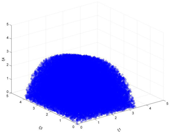
Figure 1.
The market stability domain (, emission reduction target: 16%).
Similarly, when the target increases from 17% to 20%, the steel market stability domain composed of ξ1, ξ3, and ξ4 is basically the same as when the target is 15%.
When the target is 16%, ξ2, ξ5, and ξ6 increase from 1.00 to 5.00 (Figure 2); it can be seen that as the northeast, southwest, and northwest regions adopt positive production adjustment coefficients at the same time, the stability of the steel market gradually decreases. The changing trend of the shape of the stability region is very similar to that when the target is 15%. When ξ2, ξ5, and ξ6 are large, the other three regions still have sufficient room for output adjustment.
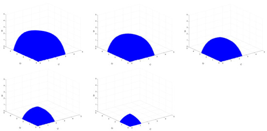
Figure 2.
The market stability domain (, emission reduction target: 16%).
However, it should be pointed out that when the target is small, the change in the stable region is almost unchanged. However, with the gradual increase in the target (take 20% as an example), the difference in the area of the stable region becomes more obvious. Take the emission reduction targets of 15% and 20%, respectively, when ξ2, ξ5, and ξ6 are set to 5 at the same time as an example; the results are shown in Figure 3.
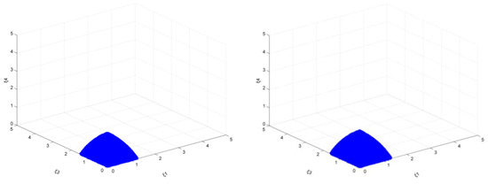
Figure 3.
The market stability domain (, emission reduction target: left 15%, right 20%).
The value range of ξ1 is increased from [0, 1.275] to [0, 1.325], the value range of ξ3 is increased from [0, 1.500] to [0, 1.600], and the value range of ξ4 is increased from [0, 1.900] to [0, 2.025]. Judging from the results, the area of the stability region shows an increasing trend as the target increases. It shows that under the combined effect of the carbon tax and the output adjustment policy of smaller output enterprises, the larger output enterprises’ output adjustment policies will show an increasing trend.
- The output adjustment speed of ξ1, ξ3, ξ4 remains unchanged
As the emission reduction target is 16% (previous research has analyzed the results when the target is 15%), and ξ1, ξ3, ξ4 are both set to 0, the steel market stability domain composed of ξ2, ξ5, and ξ6 is analyzed. As can be seen in Figure 4, the range of ξ2 is [0, 10.00], ξ5 is [0, 7.50], ξ6 is [0, 10.00], or even more. The value range of ξ considered in this section is [0, 10], which is basically the same as the result when the target is 15%.
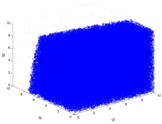
Figure 4.
The market stability domain (, emission reduction target: 16%).
Similarly, when the target is gradually increased from 17% to 20%, the market stability domain composed of ξ2, ξ5, and ξ6 is basically the same as when the target is 15%.
When the target is 16%, ξ1, ξ3, and ξ4 simultaneously increase from 0.50 to 2.00 (Figure 5), it can be seen that when the North, East, and South Central China adopt positive production adjustment coefficients at the same time, the stability of the steel market gradually decreases. It can be clearly found that when ξ1, ξ3, ξ4 take small positive values, Northeast China, Southwest China, and Northwest China still have greater autonomy in decision-making. However, when ξ1, ξ3, ξ4 gradually increase, the stable area of the entire steel market will shrink sharply. When ξ1, ξ3, ξ4 are 2, the value range of ξ2, ξ5, ξ6 is very small. Obviously, when ξ1, ξ3, ξ4 keep increasing, the market is easily out of balance.
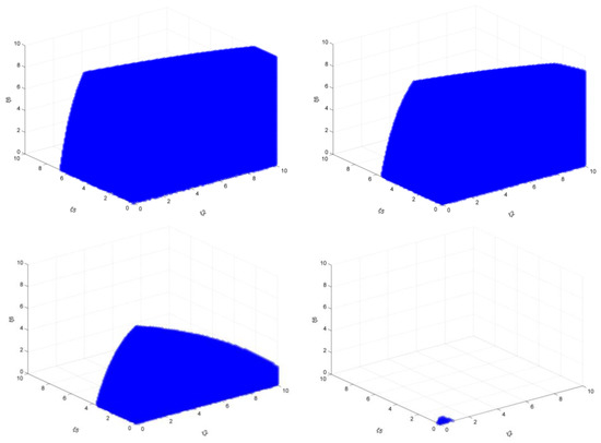
Figure 5.
Stability domain of the market (, emission reduction target: 16%).
Similarly, the shape and change trends of the stable region are very similar, and when the target is small (close to 15%), the change in the stable region is almost unchanged. However, when the target is high (take 20% as an example), the difference in the area of the stable region becomes more obvious. Take the emission reduction targets of 15% and 20%, respectively, and when ξ1, ξ3, and ξ4 take 1.5 at the same time as an example, the results are shown in Figure 6.
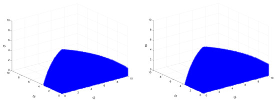
Figure 6.
The market stability domain (, emission reduction target: left 15%, right 20%).
The value range of ξ2 is still maintained at [0, 10] (but through further calculations, the upper limit is increased), the value range of ξ5 is increased from [0, 3.60] to [0, 3.70], the value range of ξ6 is increased from [0, 8.80] to [0, 9.20]. Judging from the results, the area of the stability region shows an increasing trend as the target increases. It means that under the combined effect of the single carbon tax and larger output enterprises’ output adjustment policies, the smaller output enterprises’ output adjustment policies will also increase.
- System dynamic characteristics analysis
According to the previous research, this section selects two groups of representative enterprises: North China (representing larger output enterprises) and Southwest China (representing smaller output enterprises). Therefore, in this section, we will discuss ξ1, ξ5 and the change impacts on system stability (we actually calculated all the results with a reduction target of 15–20%, but due to space limitations, this section uses a reduction target of 20% as an example). The results are shown in Figure 7, Figure 8, Figure 9 and Figure 10.
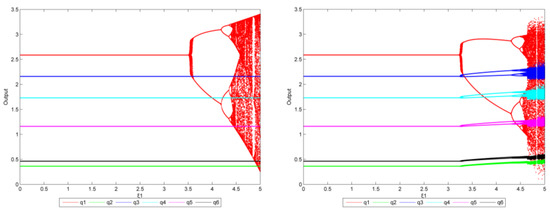
Figure 7.
The bifurcation diagram of (left: = 0, right: = 0.4, the reduction target is 20%).
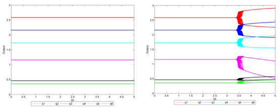
Figure 8.
The bifurcation diagram of (left: = 0, right: = 1.5, the reduction target is 20%).
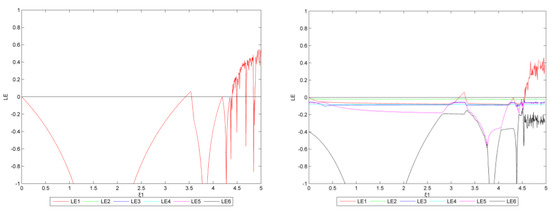
Figure 9.
The Lyapunov exponent diagram (left: = 0, right: = 0.4, the reduction target is 20%).
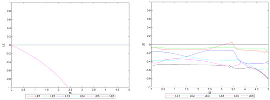
Figure 10.
The Lyapunov exponent diagram (left: = 0, right: = 1.5, the reduction target is 20%).
From Figure 7, some results can be obtained: when = 0 (left), the system is stable as is in the range of [0, 3.520]. Then, there is a small interval in which is unstable. When the value increases to 3.530, the system is no longer balanced and transitions from stable to double-cycle to chaos, but only North China has an output imbalance. When = 0.4 (right), the system is stable as is below 3.265. There is then a small interval in which production is unstable. When the value increases to 3.270, the system is no longer balanced and transitions from stable to double-cycle to chaos. However, the output of other regions appears unbalanced as gradually increases.
This shows that the system is more likely to fall into an unbalanced state when multiple enterprises use dynamic output adjustment at the same time instead of a single enterprise adopting output adjustment. Compared with the previous study (the target is 15%), the bifurcation value of has increased (the results of the first bifurcation in the previous study are 3.230 and 3.250, respectively), which also verifies this conclusion: as the emission reduction target gradually increases, enterprises with a larger output can implement more adjustment policies without causing the system to fall into a state of bifurcation or even chaos.
From Figure 8, when = 0 (left), the system remains in equilibrium regardless of . When are at 1.5 (right), the system is stable as is below 3.395. There is then a small interval in which all enterprises’ production is unstable. When the value increases to 3.410, the system is no longer balanced and transitions from stable to double-cycle to chaos. Similarly, compared with the previous study (the target is 15%), the bifurcation value of has increased (the results of the bifurcation for the first time in the previous study was 3.100), which also verifies the following conclusion: as the emission reduction target gradually increases, enterprises with smaller output can also implement more output adjustment policies without causing the system to fall into a state of bifurcation or even chaos.
From the results of Figure 7 and Figure 8, the larger output enterprises can have a much greater impact on the system balance than those smaller output enterprises, and misadjusted adjustment of output by these larger producers will easily create market imbalance. With the gradually increasing emission reduction targets, the enterprises’ policies of output adjustment could be more flexible and diverse, and the system will be in a state of bifurcation and chaos.
Figure 9 and Figure 10 show the Lyapunov exponents for Figure 7 and Figure 8. When = 0 and = 3.520 (left in Figure 9), the system shows bifurcation. When > 4.395, the maximum Lyapunov exponent changes from negative to positive, and the system is in chaos. When are 0.4 and = 3.265 (right in Figure 9), bifurcation appears and then all enterprises bifurcate. When > 4.545, the maximum Lyapunov exponent changes from negative to positive, and the system becomes chaotic.
When are 0 (left in Figure 10), the maximum Lyapunov exponent is always negative. When equal 1.5 (right in Figure 10) and range from 3.095 to 3.450, the maximum Lyapunov exponent changes from negative to positive, and there are bifurcations in various regions. When > 3.455, the maximum Lyapunov exponent is no longer positive, while the system becomes double-cycle.
4.2.2. Mixed Carbon Tax Policy Scenario in 2025: Carbon Tax + Subsidy
In this scenario, the equilibrium output E* of each regional enterprise with different emission reduction targets are as shown in Table 7.

Table 7.
The equilibrium output E* of each regional enterprise (emission reduction target: 20–25%).
And the Jacobian matrix J obtained are as shown in Table 8.

Table 8.
The Jacobian matrix J (emission reduction target: 20–25%).
In order to facilitate discussion and save space, this section only discusses the relevant calculation results under the scenarios of 20% and 25% emission reductions.
- The output adjustment speed of ξ2, ξ5, ξ6 remains unchanged
As the emission reduction target is 20%, and ξ2, ξ5, and ξ6 take 0 at the same time, the steel market stability domain composed of ξ1, ξ3, and ξ4 is analyzed. As can be seen in Figure 11, the adjustment coefficient ξ1 range is [0, 3.50], ξ3 range is [0, 4.05], and ξ4 range is [0, 4.80].
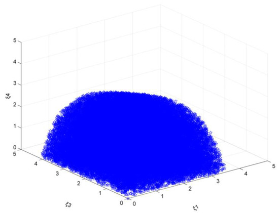
Figure 11.
The market stability (, emission reduction target: 20%).
When the target is 20%, ξ2, ξ5, ξ6 change from 1.00 to 5.00 (Figure 12), and the stable area is gradually decreasing. The changing trend of its shape is very similar to that of a single carbon tax policy. However, the difference is that when the values of ξ2, ξ5, and ξ6 are large (=4), there is still room for output adjustment in the other three regions, but compared to only a single carbon tax scenario, the area of its stability region has been greatly reduced, but when ξ2, ξ5, and ξ6 continue to increase to 5, there is not much stability in the region left. It means that with the introduction of the mixed emission reduction policies, enterprises’ output adjustment policies have been compressed, and enterprises with larger output have to carefully consider their next production strategy to avoid the entire steel market falling into an imbalance.
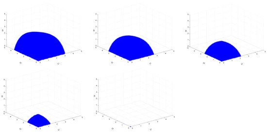
Figure 12.
The market stability domain (, emission reduction target: 20%).
On the other hand, the area difference of the stability region becomes more obvious when the targets gradually increase. For a clear comparison, this part takes emission reduction targets of 20% and 25%, respectively, when ξ2, ξ5, and ξ6 are set to 5 at the same time as an example, as shown in Figure 13.
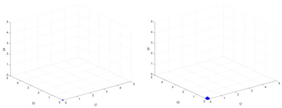
Figure 13.
The market stability domain (, emission reduction target: left 20%, right 25%).
From Figure 13, the stability domain, which is almost nonexistent, becomes significantly larger when the target increases from 20% to 25%. The value range of ξ1 is expanded to [0, 0.125], the value range of ξ3 is expanded to [0, 0.150], and the value range of ξ4 is expanded to [0, 0.200]. This shows that even if there is a mixed emission reduction policy, under the combined effect of the emission reduction policy and the output adjustment policy of an enterprise with a smaller output, as the target gradually increases, the output adjustment policies that enterprises with larger output will show an increasing trend.
- The output adjustment speed of ξ1, ξ3, ξ4 remains unchanged
As the emission reduction target is 20%, and ξ1, ξ3, and ξ4 are taken as 0 at the same time, the steel market stability domain composed of ξ2, ξ5, and ξ6 is analyzed. As can be seen in Figure 14, the adjustment coefficient ξ2 range is [0, 9.50], ξ5 range is [0, 7.50], and ξ6 range is [0, 10.00], or even more.
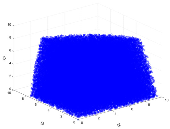
Figure 14.
The market stability domain (, emission reduction target: 20%).
Figure 15 shows that when the target is 20%, the steel market stability domain of ξ1, ξ3, and ξ4 increase from 0.50 to 2.00.
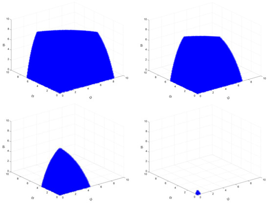
Figure 15.
The market stability domain (, emission reduction target: 20%).
From the results, the stability domain is gradually decreasing, but the difference is that the decrease in the area of the stability region under this scenario is even more dramatic. For example, when ξ1, ξ3, and ξ4 take 1.5, the output adjustment space of the other three regions is as follows: ξ2 is [0, 4.70], ξ5 is [0, 3.70], ξ6 is [0, 9.20]; compared to only a single carbon tax scenario (the target is 20%), the area of its stability area has been greatly reduced. When the values of ξ1, ξ3, and ξ4 are larger, it is foreseeable that the moment of system imbalance will be earlier than in the situation where there is only a single carbon tax policy scenario (the target is 20%).
Similarly, when the target is increased from 20% to 25%, when ξ1, ξ3, and ξ4 take 1.5 at the same time, the value range of ξ2 is increased from [0, 4.70] to [0, 4.80], the value range of ξ5 is maintained at [0, 3.70], and the value range of ξ6 is increased from [0, 9.20] to [0, 9.40]. When ξ1, ξ3, and ξ4 take other smaller values, there is a similar rule. However, when ξ1, ξ3, and ξ4 take larger values at the same time (and there is a stable region), the conclusion is different. When the target increases from 20% to 25%, ξ1, ξ3, and ξ4 take 2, and the value range of ξ2 and ξ5 is maintained in the interval of [0, 0.40] and [0, 0.30], but the value range of ξ6 is reduced from [0, 0.80] to [0, 0.70]. These results are shown in Figure 16 and Figure 17.

Figure 16.
The market stability domain (, emission reduction target: left 20% (2020), middle 20% (2025), right 25%).

Figure 17.
The market stability domain (, emission reduction target: left 20% (2020), middle 20% (2025), right 25%).
This illustrates that when the government adopts a mix of emission reduction policies, under the combined effect of these policies and output adjustment policy of the larger output enterprise, the smaller output enterprise adjustment policy will be restricted or affected by more factors. The rule of change is different from that of a single carbon tax scenario, which means that enterprises with smaller outputs need to be more cautious in formulating their own production plans to ensure that the enterprises themselves and the entire steel market will not fall into an imbalanced state.
- System dynamic characteristics analysis
In this section, we have calculated all the results with a reduction target of 20–25%, but due to space limitations, this section uses a reduction target of 25% as an example for discussion.
From Figure 18, some results can be obtained: when = 0 (left), the system is stable as is in the range of [0, 3.625]. Then, there is a small interval wherein is unstable. When the value increases to 3.630, the system is no longer balanced and transitions from stable to double-cycle to chaos, but only North China has an output imbalance. When = 0.4 (right), the system is stable as is below 3.345. Then, there is a small interval in which the production is unstable. When the value increases to 3.350, the system is no longer balanced and transitions from stable to double-cycle to chaos. However, the output of other regions appears unbalanced as gradually increases.
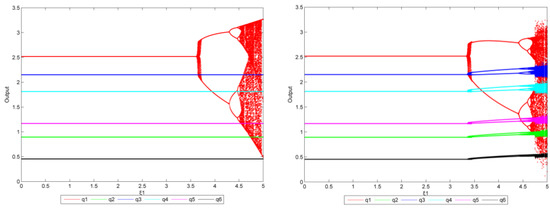
Figure 18.
The bifurcation diagram of (left: = 0, right: = 0.4, the reduction target is 25%).
From Figure 19, when = 0 (left), the system remains in equilibrium regardless of . When are at 1.5 (right), the system is stable as is below 2.950. Then, there is a small interval in which all enterprises’ production is unstable. When the value increases to 2.970, the system is no longer balanced and transitions from stable to double-cycle to chaos.
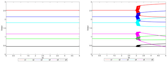
Figure 19.
The bifurcation diagram of (left: = 0, right: = 1.5, the reduction target is 25%).
Figure 20 and Figure 21 show the Lyapunov exponents for Figure 18 and Figure 19. When = 0 and = 3.625 (left in Figure 20), the system shows bifurcation. When > 4.505, the maximum Lyapunov exponent changes from negative to positive, and the system is in chaos. When are 0.4 and = 3.345 (right in Figure 20), bifurcation appears and then all enterprises bifurcate. When > 4.655, the maximum Lyapunov exponent changes from negative to positive, and the system becomes chaotic.
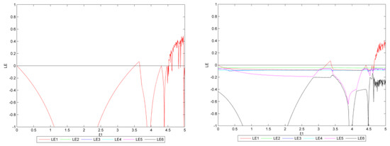
Figure 20.
The Lyapunov exponent diagram (left: = 0, right: = 0.4, the reduction target is 25%).
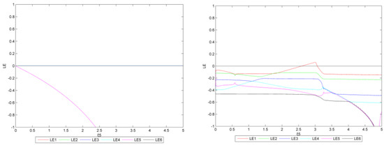
Figure 21.
The Lyapunov exponent diagram (left: = 0, right: = 1.5, the reduction target is 25%).
When are 0 (left in Figure 21), the maximum Lyapunov exponent is always negative. When equal 1.5 (right in Figure 21) and range from 2.590 to 3.060, the maximum Lyapunov exponent changes from negative to positive, and there are bifurcations in various regions. When > 3.065, the maximum Lyapunov exponent is no longer positive, while the system becomes double-cycle.
4.2.3. Multiple Mixed Carbon Tax Policy Implemented in 2030: Carbon Tax + Subsidy + CCS
In this scenario, the equilibrium output E* of each regional enterprise with different emission reduction targets are as shown in Table 9.

Table 9.
The equilibrium output E* of each regional enterprise (emission reduction target: 25–30%).
And the Jacobian matrix J obtained are as shown in Table 10.

Table 10.
The Jacobian matrix J (emission reduction target: 25–30%).
In order to facilitate discussion and save space, this section only discusses the relevant calculation results under the scenarios of 25% and 30% emission reductions.
- The output adjustment speed of ξ2, ξ5, ξ6 remains unchanged
As the emission reduction target is 25%, and ξ2, ξ5, and ξ6 take 0 at the same time, the steel market stability domain composed of ξ1, ξ3, and ξ4 is analyzed. As can be seen in Figure 22, the adjustment coefficient ξ1 range is [0, 3.60], ξ3 range is [0, 4.15], and ξ4 range is [0, 5.00].
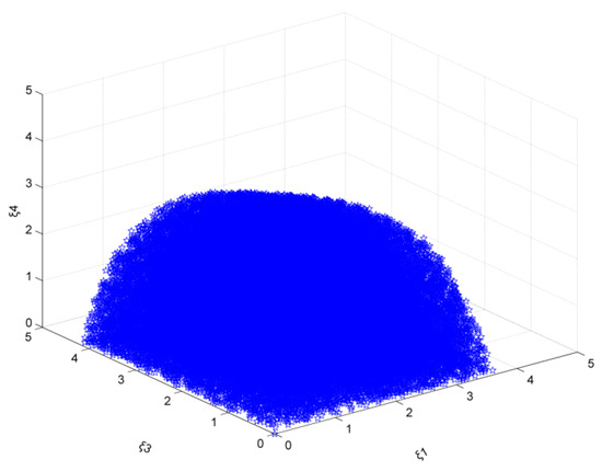
Figure 22.
The market stability domain (, emission reduction target: 25%).
When the target is 25%, ξ2, ξ5, and ξ6 change from 1.00 to 4.00 (Figure 23), and the stable area is gradually decreasing. The changing trend of its shape is very similar to that of the mixed carbon tax policy (carbon tax+ subsidy, scenario 2025). However, the difference is that when the values of ξ2, ξ5, and ξ6 are large (=4), there is still room for output adjustment in the other three regions, but compared to the mixed carbon tax policy scenario (emission reduction target = 25%), the area of its stability region has been greatly reduced; when ξ2, ξ5, and ξ6 continue to increase to 5, there is no longer a stable region. It means that with the implementation of multiple emission reduction policies, enterprises with larger output have to carefully consider their next production strategies to avoid output adjustment strategies that would spur the entire steel market into imbalance.
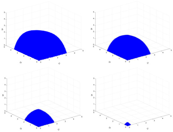
Figure 23.
The market stability domain (, emission reduction target: 25%).
On the other hand, the area difference of the stability region becomes more obvious when the targets gradually increase. For a clear comparison, this part takes emission reduction targets of 25% and 30%, respectively, when ξ2, ξ5, and ξ6 are taken as 4 at the same time as an example, as shown in Figure 24.
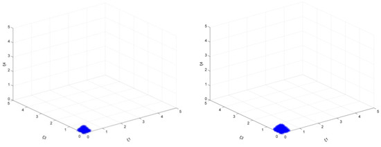
Figure 24.
The market stability domain (, emission reduction target: left 25%, right 30%).
As shown in Figure 24, the stability domain, which is very small, became significantly larger when the target increases from 25% to 30%. The value range of ξ1 is increased from [0, 0.35] to [0, 0.45], the value range of ξ3 is increased from [0, 0.45] to [0, 0.50], and the value range of ξ4 is increased from [0, 0.50] to [0, 0.60]. This also shows that even if there are more complex mixed emission reduction policies, under the combined effect of the emission reduction policy and the output adjustment policy of an enterprise with a smaller output, as the target gradually increases, the output adjustment policies that enterprises with larger output will show an increasing trend.
- The output adjustment speed of ξ1, ξ3, ξ4 remains unchanged
As the emission reduction target is 25% and ξ1, ξ3, and ξ4 are taken as 0 at the same time, the steel market stability domain composed of ξ2, ξ5, and ξ6 is analyzed. As can be seen in Figure 25, the adjustment coefficient ξ2 range is [0, 8.30], ξ5 range is [0, 6.30], ξ6 range is [0, 10.00], or even more, which is smaller than the scenario of carbon tax+ subsidy policy with an emission reduction target of 25%. This suggests that when introducing the multiple emission reduction policies, production plans of enterprises with smaller output will be affected more obviously.
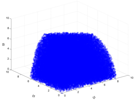
Figure 25.
The market stability domain (, emission reduction target: 25%).
Figure 26 shows that when the target is 25%, the steel market stability domain of ξ1, ξ3, and ξ4 increases from 0.50 to 2.00.
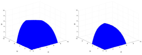
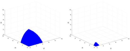
Figure 26.
The market stability domain (, emission reduction target: 25%).
From the results, the overall stability domain shows a gradual decreasing trend, but compared with the previous, the conclusion is slightly different. For example, when ξ1, ξ3, and ξ4 take 1.5, the output adjustment space of the other three regions is as follows: ξ2 is [0, 4.40], ξ5 is [0, 3.30], ξ6 is [0, 6.90]; compared to the scenario of carbon tax+ subsidy (emission reduction target of 25%), the area of its stability area has been greatly reduced. However, when the values of ξ1, ξ3, and ξ4 are larger (=2), the area of the stability region is larger than the scenario of the carbon tax+ subsidy (the target is 25%). When ξ1, ξ3, and ξ4 continue to increase, the system will enter a state of imbalance, but the moment of system imbalance will be later than the scenario of the carbon tax+ subsidy (the target is 25%).
Similarly, when the target increases from 25% to 30% and when ξ1, ξ3, and ξ4 take 1.5 at the same time, the value range of ξ2 is increased from [0, 4.40] to [0, 4.50], the value range of ξ5 is maintained at [0, 3.30], and the value range of ξ6 is maintained at [0, 6.90]. When ξ1, ξ3, and ξ4 are other smaller values, there is a similar rule. However, when ξ1, ξ3, and ξ4 take larger values at the same time (and there is a stable region), the conclusion is different. When the target is increased from 25% to 30%, and when ξ1, ξ3, and ξ4 take 2 at the same time, the value range of ξ2 is maintained in the interval of [0, 1.10], but the value range of ξ5 is reduced from [0, 0.80] to [0, 0.70], and the value range of ξ6 is reduced from [0, 1.60] to [0, 1.50]. These results are shown in Figure 27 and Figure 28.

Figure 27.
The market stability domain (, emission reduction target: left 25% (2025), middle 25% (2030), right 30%).

Figure 28.
The market stability domain (, emission reduction target: left 25% (2025), middle 25% (2030), right 30%).
This also shows that with the implementation of more complex mixed emission reduction policies, under the combined effect of emission reduction policies and output adjustment policies of larger output enterprises, the smaller output enterprise adjustment policy will be restricted by more factors. The rule of change is different from that of a single carbon tax scenario. This means that enterprises with smaller outputs need to be more cautious in formulating their own production plans to ensure that the enterprises themselves and the entire steel market will not fall into an unbalanced state.
- System dynamic characteristics analysis
In this section, we have actually calculated all the results where the emission reduction target is 25–30%, but due to space limitations, this section takes the emission reduction target of 30% as an example for discussion.
From Figure 29, some results can be obtained: when = 0 (left), the system is stable as is in the range of [0, 3.730]. There is then a small interval where is unstable. When the value increases to 3.735, the system is no longer balanced and transitions from stable to double-cycle to chaos, but only North China has output imbalance. When = 0.4 (right), the system is stable as is below 3.415. There is then a small interval in which production is unstable. When the value increases to 3.420, the system is no longer balanced and transitions from stable to double-cycle to chaos. However, the output of other regions appears unbalanced as gradually increases.
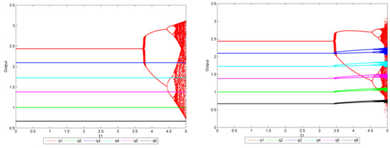
Figure 29.
The bifurcation diagram of (left: = 0, right: = 0.4, the reduction target is 30%).
From Figure 30, when = 0 (left), the system remains in equilibrium regardless of . When are at 1.5 (right), the system is stable as is below 2.450. There is then a small interval in which all enterprises’ production is unstable. When the value increases to 2.465, the system is no longer balanced and transitions from stable to double-cycle to chaos.
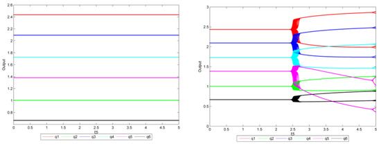
Figure 30.
The bifurcation diagram of (left: = 0, right: = 1.5, the reduction target is 30%).
Figure 31 and Figure 32 show the Lyapunov exponents for Figure 29 and Figure 30. When = 0 and = 3.730 (left in Figure 31), the system shows bifurcation. When > 4.655, the maximum Lyapunov exponent changes from negative to positive, and the system is in chaos. When are 0.4 and = 3.415 (right in Figure 31), bifurcation appears and then all enterprises bifurcate. When > 4.805, the maximum Lyapunov exponent starts to be positive, and the system becomes chaotic.
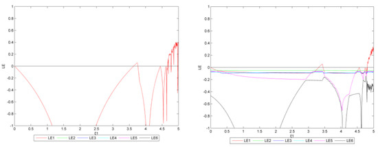
Figure 31.
The Lyapunov exponent diagram (left: = 0, right: = 0.4, the reduction target is 30%).
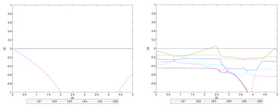
Figure 32.
The Lyapunov exponent diagram (left: = 0, right: = 1.5, the reduction target is 30%).
When are 0 (left in Figure 32), the maximum Lyapunov exponent is always negative. When equal 1.5 (right in Figure 32) and ranges from 2.165 to 2.535, the maximum Lyapunov exponent changes from negative to positive, and there are bifurcations in various regions. When > 2.540, the maximum Lyapunov exponent is no longer positive, while the system becomes double-cycle.
4.3. Further Discussions
Different from the author’s previous research [38], this paper calculates the changes in various indicators in the steel market under multiple emission reduction policies and multiple emission reduction targets, and makes corresponding comparisons. This paper does not discuss the optimal emissions intensity. Only the aforementioned three scenarios were analyzed. Moreover, because of certain assumptions in the model, there were some gaps between the calculations and the actual results, but some trends and rules can still be found and identified.
From the calculation results, it can be found that the optimal output obtained by the output selection model of the iron and steel industry is the equilibrium output under the condition of market stability. In terms of production areas, the optimal output obtained by the model is also consistent with the current basic distribution of China’s steel industry. That is to say, the optimal output in North China, East China, and Central and South China is much larger than that in other regions, and its impact on the market and production adjustment strategies have always been the focus of government departments. In other regions, because of its low market share, the impact on the market is not obvious. Therefore, in order to make the research conclusions more comparative and representative, the research on the changes in emission reduction targets, the research on the combination of emission reduction policies, and the research on production adjustment strategies are all based on the two major areas with large output (North China, Northeast China, Central South China) and areas with small production (Northeast China, Southwest China, Northwest China).
For the optimal output of the model, the author’s previous research has carried out detailed calculations; this paper does not discuss it, but focuses on the impact of the adjustment of bounded rational production strategies in various regions of the steel market.
In general, changes in the production adjustment strategies of enterprises directly affect the stability of the steel market. Whether the enterprise with a large output or with a small output, excessive production adjustment strategies will affect the stability of the market. However, the possibility of market imbalance is very small (the unit of production adjustment strategy in this paper is 100 million tons, which is almost impossible for enterprises and is almost completely “unreasonable” only for more obvious and outstanding results and calculated). Therefore, for enterprises, the research on the combination of carbon emission reduction goals and carbon emission reduction strategies affects the production decisions of enterprises to a certain extent.
For North China, East China, and Central South China, since their steel production bases will not be fundamentally relocated and eliminated for a long period of time in the future, their market share will still occupy a considerable proportion. From the calculation results, the increase in CO2 emission reduction targets affects the output of North China, East China, and Central South China but increases the production adjustment strategy of these regions, that is, they can adopt more flexible production plans. Obviously, under the dual carbon goal, it is most important for steel enterprises in these regions to complete the corresponding emission reduction plans (the requirements of emission reduction policy combination can be ignored to a certain extent). Previous studies [14,44,54] have conducted corresponding studies on the choice of CO2 emission reduction strategies.
For the northeast, southwest and northwest regions, although the possibility of market imbalance is also less, it cannot be ruled out that due to the low market share and poor profits of these enterprises, the decision makers of these enterprises may take “life-threatening” expansion of production, and the final result will cause market imbalance. Of course, in most cases, the production adjustment plans of iron and steel enterprises in the Northeast, Southwest, and Northwest regions are relatively stable. Therefore, under the dual carbon goal, for iron and steel enterprises in the northeast, southwest, and northwest regions, implementing a simple combination of CO2 emission reduction policies is more conducive to market stability and the realization of emission reduction goals.
5. Research Conclusions and Recommendations
This paper constructs a repeated dynamic game model and introduces the carbon tax mechanism and bounded rationality expectation strategy. Then the output selection and market stability of steel oligarchs under multiple emission reduction targets and policies are analyzed, and the dynamic production adjustment and market imbalance conditions of steel oligarchs under various conditions, as well as the corresponding stability regions, bifurcation diagrams, and Lyapunov exponent are further analyzed and compared. This research draws the following conclusions.
When the industry implements a single or mixed carbon tax policy and output adjustment policy, the market stability domain, and system dynamics characteristics are basically similar to the previous research conclusions. That is, the system balance influence of larger output enterprises is much greater than that of smaller output enterprises. When larger output enterprises adopt weak positive adjustment policies, smaller output enterprises will have more autonomy in output planning. However, when large-scale enterprises adopt improper output adjustment policies, such as an excessive output, it is more dangerous for small-scale enterprises as it will cause their output adjustment space to shrink sharply. In addition, when multiple firms simultaneously employ dynamic output adjustments, the system is more prone to falling into an imbalanced state.
When output adjustment policy and a single carbon tax policy are combined to act on the steel market, as emission reduction targets are gradually raised, the adjustment policies that enterprises with larger or smaller output can implement will show an increasing trend, that is, enterprises can implement more output adjustment policies without causing the system to fall into a state of bifurcation or even chaos.
However, if the emission reduction target it consistently raised and the carbon tax policy adds subsidies, CCS, and other mixed emission reduction policies, the conclusion is slightly different. For enterprises with a larger output, even if a more complex mixed emission reduction policy appears, as the target gradually increases, the output adjustment policies that can be implemented will also show an increasing trend. However, for enterprises with smaller output, the output adjustment policy will be restricted and affected by more factors including emission reduction targets. The rule of change is different from that of the single carbon tax scenario, and it even occurs that the stability zone shrinks and the output adjustment policies decrease when the emission reduction target is large. This means that enterprises with smaller output need to be more cautious in formulating their own production plans to ensure that the enterprises themselves and the entire steel market will not fall into a state of imbalance.
Based on the above research analysis, some relevant and reasonable suggestions are put forward for the steel industry’s high-quality development of transformation and improvement: the government and enterprises need to consider all factors and differences between enterprises when formulating future production plans. Enterprises with a larger output and larger market share can take more flexible choices in the process of output adjustment; however, enterprises with a smaller output and smaller market share should not adjust their output plans significantly in the process of output adjustment and should observe the output changes in enterprises with a larger output and make corresponding adjustments. When the steel industry implements more stringent emission reduction targets and policies in the future, the department should pay close attention to the adjustment of output plans of various enterprises (especially those with small output) at any time and beware of malicious production, disruption of market competition order, and market imbalance. In short, carbon tax, hybrid emission reduction policies, and output adjustment strategies (including the product differentiation strategies studied previously) have their own reasonable scope of application. The government and enterprises should carefully weigh these strategic issues in their output plans.
Author Contributions
Conceptualization, D.L. and Y.D.; methodology, Y.D.; software, D.Z. and Y.D.; validation, D.Z. and Y.D.; formal analysis, D.Z. and Y.D.; investigation, Y.D.; resources, Y.D; data curation, Y.D.; writing—original draft preparation, D.L. and Y.D.; writing—review and editing, Q.D., Z.H. and H.Z.; visualization, D.Z. and Y.D.; supervision, Y.D.; project administration, Y.D.; funding acquisition, Y.D. All authors have read and agreed to the published version of the manuscript.
Funding
The authors gratefully acknowledge the financial support from the Social Science Foundation of Liaoning Province [L19CJY006]. These will be used for the purchase and collection of information and data, as well as for the modification and publication of the manuscript.
Data Availability Statement
The statistics in this paper are from the China Statistical Yearbook, China Industrial Statistical Yearbook, China Energy Statistical Yearbook, China Steel Yearbook, and the statistical yearbooks of various provinces. All data are publicly available on the website and can also be purchased. The relevant results of this paper are calculated on the basis of these public data, and these statistical data and books have been marked and quoted in the paper.
Acknowledgments
The author of this paper thanks the School of Geography of Liaoning Normal University for their assistance in developing this research.
Conflicts of Interest
The authors declare no conflict of interest.
Appendix A
The detailed solution and derivation process of the variation range of ξi (i = 1, 2, 3, 4, 5, 6):
When , there are:
Among these results, a Nash equilibrium point can be obtained. The stability linear discrete system can be judged by the eigenvalues of its Jacobian matrix. First, calculate its Jacobian matrix J,
where
Then the characteristic equation at the equilibrium point of the Jacobian matrix is:
where
and
Then the stable domain of the market can be obtained.
References
- Mann, R.F. The Case for the Carbon Tax: How to Overcome Politics and Find Our Green Destiny. Environ. Law Report. 2009, 39, 10118–10126. [Google Scholar]
- Wu, L.Y.; Wang, Z.; Xu, C.J.; Yan, Y.M. A CGE Model for Provincial Carbon Economy: A Case Study of Henan Province. Geogr. Res. 2016, 35, 941–952. [Google Scholar]
- Wang, F.; Chen, J.G.; Liu, J.; Lin, X.Y.; Chen, S. Effect of Carbon Tax on Macro-Economy and Carbon Emission Reduction in Jiangsu Province: Simulation Analysis Based on CGE Model. Ecol. Econ. 2017, 33, 31–36. [Google Scholar]
- Yahoo, M.; Othman, J. Employing a CGE model in analysing the environmental and economy-wide impacts of CO2 emission abatement policies in Malaysia. Sci. Total Environ. 2017, 584–585, 234–243. [Google Scholar] [CrossRef] [PubMed]
- Li, Y.; Su, B. The impacts of carbon pricing on coastal megacities: A CGE analysis of Singapore. J. Clean. Prod. 2017, 165, 1239–1248. [Google Scholar] [CrossRef]
- Qiao, H.; Song, N.; Gao, H.W. Analysis on the Strategies of European Union’s Airline Carbon Tax with Stackelberg Game Models. Syst. Eng. Theory Pract. 2014, 34, 158–167. [Google Scholar]
- Xu, X.Y.; Xu, X.P.; He, P. Joint Production and Pricing Decisions for Multiple Products with Cap-and-Trade and Carbon Tax Regulation. J. Clean. Prod. 2016, 112, 4093–4106. [Google Scholar] [CrossRef]
- Cao, K.Y.; Xu, X.P.; Wu, Q.; Zhang, Q.P. Optimal Production and Carbon Emission Reduction Level under Cap-and-Trade and Low Carbon Subsidy Policies. J. Clean. Prod. 2017, 167, 505–513. [Google Scholar] [CrossRef]
- Mathiesen, L.; Maestad, O. Climate Policy and the Steel Industry: Achieving Global Emission Reductions by an Incomplete Climate Agreement. Energy J. 2004, 25, 91–114. [Google Scholar] [CrossRef]
- Liang, Q.-M.; Fan, Y.; Wei, Y.-M. The effect of energy end-use efficiency improvement on China’s energy use and CO2 emissions: A CGE model-based analysis. Energy Effic. 2009, 2, 243–262. [Google Scholar] [CrossRef]
- Nie, H.L.; Zhou, J.P.; Zhang, H. Optimization Choices of Carbon Tax Policies for Energy Enterprises Based on Effects of Carbon Emissions Reduction. Resour. Sci. 2011, 33, 1906–1913. [Google Scholar]
- Kuo, T.C.; Hong, I.H.; Lin, S.C. Do carbon taxes work? Analysis of government policies and enterprise strategies in equilibrium. J. Clean. Prod. 2016, 139, 337–346. [Google Scholar] [CrossRef]
- Wakiyama, T.; Zusman, E. What would be the effects of a carbon tax in Japan: A historic analysis of subsidies and fuel pricing on the iron & steel, chemical, and machinery industries. Appl. Energy 2016, 4, 606–632. [Google Scholar]
- Duan, Y.; Li, N.; Mu, H.; Gui, S. Research on CO2 Emission Reduction Mechanism of China’s Iron and Steel Industry under Various Emission Reduction Policies. Energies 2017, 10, 2026. [Google Scholar] [CrossRef]
- Duan, Y.; Han, Z.; Mu, H. Research on the influence of product differentiation and emission reduction policy on CO2 emissions of China’s iron and steel industry. Int. J. Clim. Chang. Strat. Manag. 2020, 12, 717–737. [Google Scholar] [CrossRef]
- Ntombela, S.M.; Bohlmann, H.R.; Kalaba, M.W. Greening the South Africa’s Economy Could Benefit the Food Sector: Evidence from a Carbon Tax Policy Assessment. Environ. Resour. Econ. 2019, 74, 891–910. [Google Scholar] [CrossRef]
- Li, Z.L.; Dai, H.C.; Song, J.N. Assessment of the carbon emissions reduction potential of China’s iron and steel industry based on a simulation analysis. Energy 2019, 183, 279–290. [Google Scholar] [CrossRef]
- Zhu, X.; Zeng, A.; Zhong, M.; Huang, J.; Qu, H. Multiple impacts of environmental regulation on the steel industry in China: A recursive dynamic steel industry chain CGE analysis. J. Clean. Prod. 2019, 210, 490–504. [Google Scholar] [CrossRef]
- Wu, F.; Xie, W.X. Energy consumption scenario analysis of China’s steel industry under low carbon constraints. Mod. Chem. Ind. 2019, 39, 12–17. [Google Scholar]
- Deng, L.; Adams, T.A. Comparison of steel manufacturing off-gas utilization methods via life cycle analysis. J. Clean. Prod. 2020, 277, 123568. [Google Scholar] [CrossRef]
- Liu, M.; Chen, X.; Zhang, M.; Lv, X.; Wang, H.; Chen, Z.; Huang, X.; Zhang, X.; Zhang, S. End-of-life passenger vehicles recycling decision system in China based on dynamic material flow analysis and life cycle assessment. Waste Manag. 2020, 117, 81–92. [Google Scholar] [CrossRef] [PubMed]
- Zhao, H.; Song, S.; Zhang, Y.; Liao, Y.; Yue, F. Optimal decisions in supply chains with a call option contract under the carbon emissions tax regulation. J. Clean. Prod. 2020, 271, 122199. [Google Scholar] [CrossRef]
- Ji, W.Z. Study on Outputs Game Models and Chaotic Characters in Electric Power Oligopoly. Ph.D. Thesis, Tianjin University, Tianjin, China, 2008. [Google Scholar]
- Sun, Z.H.; Ma, J.H. Game Model of Dynamically Repeated Price in Domestic Steel Market. J. Xidian Univ. Soc. Sci. Ed. 2009, 19, 43–47. [Google Scholar]
- Tu, H.L. Research on the Dynamics of the Cournot Dynamical Game Models in the Electricity Market and the Renewable Resource Market. Ph.D. Thesis, Tianjin University, Tianjin, China, 2013. [Google Scholar]
- Dang, J.-F.; Hong, I.-H. The equilibrium quantity and production strategy in a fuzzy random decision environment: Game approach and case study in glass substrates industries. Int. J. Prod. Econ. 2013, 145, 724–732. [Google Scholar] [CrossRef]
- Tan, Z.L.; Liang, Z.X. Study on Dynamic Repetition Game Model of Coal Market Price in China. Coal Econ. Res. 2016, 36, 45–48. [Google Scholar]
- Li, Q.; Liao, F.; Timmermans, H.J.P.; Zhou, J. A User Equilibrium Model for Combined Activity-travel Choice under Prospect Theoretical Mechanisms of Decision-making under Uncertainty. Transportmetrica 2016, 12, 629–649. [Google Scholar] [CrossRef]
- Di, X.; Liu, H.X.; Ban, X.J. Second best toll pricing within the framework of bounded rationality. Transp. Res. Part B Methodol. 2016, 83, 74–90. [Google Scholar] [CrossRef]
- Di, X.; Liu, H.; Zhu, S.; Levinson, D. Indifference bands for boundedly rational route switching. Transportation 2016, 44, 1169–1194. [Google Scholar] [CrossRef]
- Liu, L.W. Nonlinear Complex Dynamics of Carbon Emission Reduction Cournot Game with Bounded Rationality. Complexity 2017, 2017, 8301630. [Google Scholar]
- Yu, Y. Complexity Analysis of Taxi Duopoly Game with Heterogeneous Business Operation Models and Differentiated Products. J. Intell. Fuzzy Syst. 2017, 33, 3059–3067. [Google Scholar] [CrossRef]
- Ding, M.; Qian, Y.; Zhang, J.; He, J.; Yi, J. Defence model based on multistage dynamic game with consideration of bounded rationality against power system cascading failure. Electr. Power Autom. Equip. 2017, 37, 69–74+82. [Google Scholar]
- Zhang, J.X. Study on Competitive Game Model with Bounded Rationality Enterprise of Emissions Trading. Value Eng. 2018, 6, 101–103. [Google Scholar]
- Sang, H.Y.; Xie, X.L.; Wang, B. Ship scheme selection based on decision maker’s limited rationality. J. Dalian Marit. Univ. 2019, 45, 58–64. [Google Scholar]
- Zhang, Y.M.; Chen, W.D.; Mi, Y. Third-party remanufacturing mode selection for competitive closed-loop supply chain based on evolutionary game theory. J. Clean. Prod. 2020, 63, 121305. [Google Scholar] [CrossRef]
- Wu, F. Research on Dynamic and Complexity of Energy-Saving Investment about Multichannel and Multienergy Supply Chain. Complexity 2020, 2020, 2409636. [Google Scholar] [CrossRef]
- Duan, Y.; Han, Z.; Mu, H.; Yang, J.; Li, Y. Research on the Influence of Bounded Rationality and Product Differentiation on the Stability of Steel Industry Market. Discret. Dyn. Nat. Soc. 2020, 2020, 1828674. [Google Scholar] [CrossRef]
- Rezvani, Z.; Hudson, P. How do middle managers really make decisions within the oil and gas industry? Saf. Sci. 2021, 139, 105199. [Google Scholar] [CrossRef]
- Fan, B.; Guo, T.; Xu, R.; Dong, W. Evolutionary Game Research on the Impact of Environmental Regulation on Overcapacity in Coal Industry. Math. Probl. Eng. 2017, 2021, 5558112. [Google Scholar] [CrossRef]
- Gao, C.; Liu, S.; Yu, C.; Guo, P. External Incentive Mechanism Research on Knowledge Cooperation-Sharing in the Chinese Creative Industry Cluster. Comput. Syst. Sci. Eng. 2021, 38, 365–379. [Google Scholar] [CrossRef]
- Ma, J.; Hou, Y.; Wang, Z.; Yang, W. Pricing strategy and coordination of automobile manufacturers based on government intervention and carbon emission reduction. Energy Policy 2021, 148, 111919. [Google Scholar] [CrossRef]
- Hammond, S.F.; Gajendran, T.; Savage, D.A.; Maund, K. Unpacking the problems behind the limited green construction adoption: Towards a theoretical model. Eng. Constr. Arch. Manag. 2021, 28, 833–844. [Google Scholar] [CrossRef]
- Duan, Y.; Han, Z.; Mu, H.; Yang, J.; Li, Y. Research on the Impact of Various Emission Reduction Policies on China’s Iron and Steel Industry Production and Economic Level under the Carbon Trading Mechanism. Energies 2019, 12, 1624. [Google Scholar] [CrossRef]
- Duan, Y.; Han, Z.; Zhang, H.; Wang, H. Research on the applicability and impact of CO2 emission reduction policies on China’s steel industry. Int. J. Clim. Chang. Strat. Manag. 2021, 13, 352–374. [Google Scholar] [CrossRef]
- NBS (National Bureau of Statistics of the People’s Republic of China). China Statistical Yearbook 2005–2017; The Editorial Board of China Statistical Yearbook: Beijing, China, 2017. [Google Scholar]
- NBS (National Bureau of Statistics of the People’s Republic of China). China Industrial Economy Statistical Yearbook 2005–2017; The Editorial Board of China Industrial Economy Statistical Yearbook: Beijing, China, 2017. [Google Scholar]
- NBS (National Bureau of Statistics of the People’s Republic of China). China Energy Statistical Yearbook 2005–2017; The Editorial Board of China Energy Statistical Yearbook: Beijing, China, 2017. [Google Scholar]
- CISA (China Iron and Steel Association). China Steel Yearbook 2005–2017; The Editorial Board of China Steel Yearbook: Beijing, China, 2017. [Google Scholar]
- IPCC (Intergovernmental Panel on Climate Change). IPCC Guidelines for National Greenhouse Gas Inventories; IPCC: Bracknell, UK, 2006. [Google Scholar]
- Duan, Y.; Mu, H.; Li, N. Analysis of the Relationship between China’s IPPU CO2 Emissions and the Industrial Economic Growth. Sustainability 2016, 8, 426. [Google Scholar] [CrossRef]
- Färe, R.S.; Grosskopf, C.A.; Pasurka, J. Environmental production functions and environmental directional distance functions. Energy 2007, 32, 1055–1066. [Google Scholar] [CrossRef]
- Lee, J.D.; Park, J.B.; Kim, T.Y. Estimation of the shadow prices of pollutants with production/environment inefficiency taken into account: A nonparametric directional distance function approach. J. Environ. Manag. 2002, 64, 365–375. [Google Scholar] [CrossRef]
- Guenno, G.; Tiezzi, S. The Index of Sustainable Economics Welfare (ISEW) for Italy; Fondazione Eni Enrico Mattei: Milano, Italy, 1998. [Google Scholar]
Publisher’s Note: MDPI stays neutral with regard to jurisdictional claims in published maps and institutional affiliations. |
© 2022 by the authors. Licensee MDPI, Basel, Switzerland. This article is an open access article distributed under the terms and conditions of the Creative Commons Attribution (CC BY) license (https://creativecommons.org/licenses/by/4.0/).