Fault Detection and Identification of Furnace Negative Pressure System with CVA and GA-XGBoost

Abstract

The boiler is an essential energy conversion facility in a thermal power plant. One small malfunction or abnormal event will bring huge economic loss and casualties. Accurate and timely detection of abnormal events in boilers is crucial for the safe and economical operation of complex thermal power plants. Data-driven fault diagnosis methods based on statistical process monitoring technology have prevailed in thermal power plants, whereas the false alarm rates of those methods are relatively high. To work around this, this paper proposes a novel fault detection and identification method for furnace negative pressure system based on canonical variable analysis (CVA) and eXtreme Gradient Boosting improved by genetic algorithms (GA-XGBoost). First, CVA is used to reduce the data redundancy and construct the canonical residuals to measure the prediction ability of the state variables. Then, the fault detection model based on GA-XGBoost is schemed using the constructed canonical residual variables. Specially, GA is introduced to determine the optimal hyperparameters of XGBoost and speed up the convergence. Next, this paper presents a novel fault identification method based on the reconstructed contribution statistics, considering the contribution of state space, residual space and canonical residual space. Besides, the proposed statistics renders different weights to the state vectors, the residual vectors and the canonical residual vectors to improve the sensitivity of faulty variables. Finally, the real industrial data from a boiler furnace negative pressure system of a certain thermal power plant is used to demonstrate the ability of the proposed method. The result demonstrates that this method is accurate and efficient to detect and identify the faults of a true boiler.

1. Introduction

In China, thermal power generation has an irreplaceable role in power industry, accounting for 70% of the total annual power generation [1,2]. For the sake of saving energy and materials, thermal power plants are moving towards high parameters and large capacity. The degree of system integration and coupling in today’s plants is far more complex than that in the conventional plants [3,4]. Since the boilers of thermal power plants operate under high pressure and temperature, one small malfunction or abnormal event will result in a dramatic reduction in plant power and efficiency, even causing equipment damage or casualties [5,6]. The boiler faults in the thermal power plant are classified as electrical and mechanical faults. The electrical faults are easy to find and identify, while the mechanical faults need to be further determined via the analysis of data from different parts of the equipment [7]. The boiler is an important energy conversion unit in a thermal power plant, which is a relatively complex energy and water–gas conversion facility. In order to ensure the supply of the qualified steam to meet the needs of load changes and the safety of boiler operation, the process parameters of each part must be strictly controlled. The main controlled parameters of the boiler system are the furnace negative pressure, the drum water level, the superheated steam temperature, the superheated steam temperature and the fuel–air ratio,. The stable furnace negative pressure is key to ensure the safety of the working environment and the facilities and the economical operation of the boiler. The main task of the furnace negative pressure control system is to control the furnace negative pressure at the set value, which controls the discharge flow of the flue gas by regulating the speed of the flue induced draft fan or the opening of the moving blades [8]. The faults of one sub-system may cause catastrophic consequences for the thermal power plant [9]. The furnace negative pressure changes after the faults of the draft fan occur. If the furnace negative pressure becomes larger, the excessive furnace negative pressure will cause the flue gas to leak, the combustion to be unstable, and even the boiler to extinguish.

Data-driven fault detection methods based on multivariate statistical process monitoring (MSPM) technologies have been gained considerable development in the industrial process, such as principal component analysis (PCA) [10,11], partial least squares (PLS) [12], canonical variable analysis (CVA) [13], and Fisher discriminant analysis (FDA) [14]. They constructed the statistics by analyzing the statistical regularity among multiple variables and detected the fault by calculating the control limits of the statistics [15]. Odgaard et al. suggested that the false negatives and false positives of PCA and PLS were high even though they can be used to identify the abnormal events [16]. To improve the accuracy of detection, Yu et al. added a second threshold to the original threshold and proposed a multi-variable threshold design method based on PCA [17]. On the other hand, the present studies projected the high-dimensional data into the low-dimensional space via statistical dimension reduction techniques to retain original information and then constructed several monitoring statistics [18,19]. Li et al. detected the abnormity according to the Manhattan distance between between the samples and the center of the fault set [20]. Xia et al. constructed monitoring statistics based on the Cauchy–Schwarz difference between two samples projected by kernel entropy component analysis [21].

After detecting a fault, the MSPM technologies were further implemented to locate the variables most closely associated with the fault by calculating the contributions of the observed variables. Kourti and MacGregor used the contribution map of variables to find the faulty variables [22]. They showed that the contribution map revealed the variables most related to abnormal events to provide a basis for further investigation. Alcala proposed a reconstruction-based contribution (RBC) method [23]. Liu et al. proposed a reduction of the combined index (RCI) to eliminate the smudging effect caused by the traditional contribution plots and RBC [24,25]. Tan and Cao extended the PCA contribution method from linear system to nonlinear system [26]. The above methods are effective to identify the variables correlated with the fault, but they only measure the contributions of a sample, which is not conducive to long-term process monitoring. Zhu and Braatz proposed the method of two-dimensional contribution map [27]. Jiang et al. proposed a fault diagnosis method based on CVA, implementing two contribution graphs based on the changes in state space and the changes in residual space [28]. Since the faulty operation conditions must be different from the normal operation conditions and the faulty variables based on residual space are concerned with a new process state when a fault occurs, a higher contribution of the residual variable means that the operation condition changes and a fault occurs. The variable contribution based on residual space ties to a fault. Li et al. proposed the contribution map method based on canonical variable residuals to identify the variables associated with the faults [29].

With the development of measurement technology, thousands of sensors are used in thermal power plants, providing various types of data for process monitoring. In 2020, it was reported that 4.4ZB of data was generated, used and exchanged in industries [30]. However, this presents a challenge for fault detection and diagnosis by conducting MSPM technology due to the extensive data. The well-developed machine learning (ML) techniques provide the opportunity for fault diagnosis based on big data and a large number of scholars turn to data-driven methods based on ML, such as artificial neural network (ANN) [31], support vector machine (SVM) [32,33], etc. Moradi et al. established four data-driven classifiers based on SVM, neural network pattern recognition, adaptive neuro-fuzzy inference systems and learning vector quantization to detect abnormal events in steam generator units of once-through power plants [34]. SVM has a good capability of dealing with nonlinear and structured data due to the use of kernel function. However, the kernel function and the convex quadratic programming problem are dependent on the initialization of certain parameters. Inappropriate parameters lead to local optimization and slow convergence of SVM. A variety of optimization techniques such as genetic algorithm (GA), particle swarm optimization (PSO), and beetle antennae search algorithm (BASA) have been introduced to determine the optimal SVM parameters [35,36,37]. However, the computational burden of SVM is relatively heavy since it takes a lot of time to train the models.

To economy the computation time, the eXtreme Gradient Boosting (XGBoost) algorithm was proposed by Chen and Guestrin [38]. XGBoost becomes prevalent in fault detection and diagnosis due to its advantage of convenient calculation, fast running speed and high precision [39]. However, just like SVM, the improper hyperparameters of XGBoost make it prone to local minima and lower the prediction accuracy. The intelligent optimization algorithms have been used to solve the problem of local optimal solutions. GA is one of the most commonly used intelligent optimization algorithms, which was designed based on the evolution of organisms in nature [40]. GA has the advantages of a simple process, randomness and the ability to compare multiple individuals at one time. GA was used to optimize the hyperparameters of XGBoost intelligently, thereby improving the accuracy of prediction results [41]. However, the original data with high dimension contains redundant information and noise information, causing false detection and missing detection in practical application. The dimensionality reduction technology is used to reduce the complexity of the data and improve the detection accuracy. Zhang et al. combined random forest (RF) with XGBoost to build a data-driven fault detection framework, where RF was used to calculate the importance of features [42]. Fitriah et al. diagnosed stroke patients and improved diagnostic accuracy by combining PCA with XGBoost classification [43]. The PCA method performs well for process variables when the controlled variables are independent and identically distributed. However, the introduction of PCA can be rather challenging when there are a large number of strongly correlated process variables, which is common in power plants.

To address this problem, CVA is used to reduce the dimensionality of the original data. It takes serial correlations between the inputs and the outputs into account and selects pairs of variables by maximizing a correlation statistic. In this article, a novel fault detection and identification method based on CVA and GA-XGBoost is proposed, reducing the false rate and the flase negative rate and economizing the detection time. The introduction of CVA is used to reduce the data redundancy and find the maximum correlation between past behaviors and future behaviors. The canonical residual vector is used to quantify the difference between future measurements and past measurements and characterize the subtle changes of the process dynamics. To further improve the accuracy of XGBoost classification, GA is adopted to optimize seven important parameters of XGBoost, including learning_rate, n_estimators, max_depth, min_child_weight, subsample, colsample_bytree and gamma. After detecting a fault, it is more practical for practitioners to identify the cause of the fault. This paper proposes a fault identification method based on reconstructed contribution graph, which considers the influence of state space, residual space and canonical residual space. Specially, the proposed variable contribution adds different weights to the residual statistics $Q_{k,j}$, the state statistics $T_{k,j}$ and the canonical residual statistics $T_{k,j}^r$.

The rest of this paper is structured as follows. The boiler system is introduced in Section 2. In Section 3, the fault detection method based on CVA and GA-XGBoost is described, and a novel contribution graph-based fault identification method is proposed, which considers the influences of residual space, state space and canonical residual space. In Section 4, the actual process data of a boiler in a certain thermal power plant is used to illustrate the validity of the proposed method. Finally, conclusions are provided in Section 5.

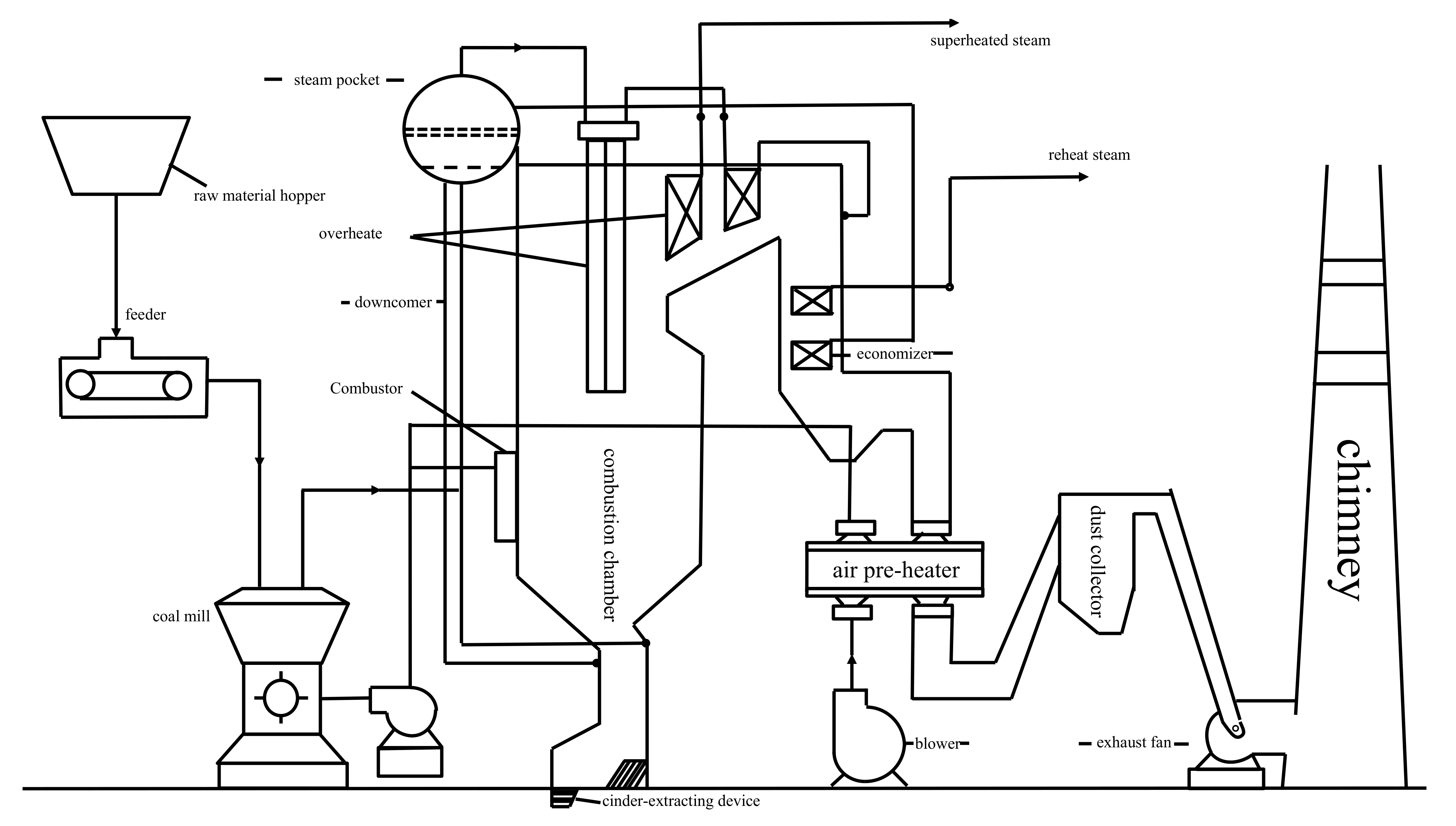
2. Background and Basic Data

Boiler is an important energy conversion equipment in thermal power plant. In the boiler, the chemical energy of the primary fuel is released by burning the coal, which is used to heat the water to raise the temperature and pressure of the water and obtain the qualified steam to meet the requirement of the turbines. As one of the three major links of the boiler, the furnace negative pressure control system plays a very important role in the normal operation of the boiler. On the premise of ensuring the safe operation of the boiler, if the furnace pressure is higher than the external atmospheric pressure, the flue gas inside the furnace will overflow. Such a case will take away a lot of heat energy and affect the boiler, the boiler-related equipment, and the personal safety of the operators and the maintenance personnel. On the contrary, if the pressure of the furnace is seriously low, the cold air outside the boiler will infiltrate into the furnace in quantity, reducing the temperature of the air entering the furnace and prolonging the ignition distance of the pulverized coal. Such case will increase the load of the exhaust fan and reduce the fuel utilization and the boiler operating efficiency.

Figure 1 presents the schematic diagram of the boiler and its auxiliary systems, which shows the main composition and operation principle of the boiler. The coal is transported to the coal yard of the thermal power plant by trains and trucks, and then transported from the coal yard to the raw coal hopper by the coal conveying belt. The raw coal is sent on demand to the coal mill through the coal feeder, where the raw coal is ground into pulverized coal. The pulverized coal is carried by the hot primary air into the furnace of the boiler and mixed with the hot secondary air for combustion. The hot flue gas formed by the pulverized coal flows along the horizontal flue and tail flue of the boiler, which flows through the full screen superheater, screen superheater, high temperature superheater, high temperature reheater, low temperature superheater, economizer and other heating surface to release heat. Then the flue gas is denitrified to remove nitrogen oxides, and then it is preheated by the air preheater to the air entering the furnace, and finally it enters the dust collector to remove dust. Under the action of draft fan, the clean flue gas is discharged into the atmosphere through the chimney, and the ash after combustion is separated by the slag removal device.

3. The Proposed Fault Detection and Identification Methodology

This section puts forward a fault detection and identification method based on CVA and GA-XGBoost. The CVA technology is used to reduce the dimensions of the original data and construct the canonical residuals from the original data. The detection model is obtained by GA-XGBoost, with the canonical residuals as input. Specially, the GA technology is used to find the optimal hyperparameters of XGBoost. Then, a novel contribution graph based the reconstructed variable contribution is proposed, considering the synthesis of the state space, the residual space and the canonical residual space.

3.1. Feature Abstraction Based on CVA

CVA extracts the canonical variables with the best predictive ability by maximizing the correlation coefficients between past space and future space. The lag of the past window is represented by p and the lag of the future window is represented by f. $n_y$ is the number of process variables. The past vector $p\left(k\right)$ and the future vector $f\left(k\right)$ are defined as:

$$\begin{array}{c}p\left(k\right)={\left[\begin{array}{cccc}{\tilde{x}}^T\left(k-1\right)& {\tilde{x}}^T\left(k-2\right)& \cdots & {\tilde{x}}^T\left(k-p\right)\end{array}\right]}^T\in R^{p{n}_y}\\ f\left(k\right)={\left[\begin{array}{cccc}{\tilde{x}}^T\left(k\right)& {\tilde{x}}^T\left(k+1\right)& \cdots & {\tilde{x}}^T\left(k+f-1\right)\end{array}\right]}^T\in R^{f{n}_y}\end{array}$$

(1)

where x stands for the process variables, and $\tilde{x}$ stands for x normalized to zero mean and unit variance. The past and future data matrices $H_p$ and $H_f$ are defined as:

$$\begin{array}{c}{H}_p=\left[\begin{array}{cccc}p\left(1\right)& p\left(2\right)& \cdots & p\left(W\right)\end{array}\right]\in R^{n_y\times W}\\ H_f=\left[\begin{array}{cccc}f\left(1\right)& f\left(2\right)& \cdots & f\left(W\right)\end{array}\right]\in R^{n_y\times W}\end{array}$$

(2)

where m represents the number of samples and $W=m-p-f+1$. Then, we can get a scaled Hankel matrix H, where $H={\left(\frac{1}{W-1}{H}_p{H}_p^T\right)}^{-1/2}\left(\frac{1}{W-1}{H}_p{H}_f^T\right){\left(\frac{1}{W-1}{H}_f{H}_f^T\right)}^{-1/2}$. By performing singular value decomposition (SVD) on H, two projection matrices J and L can be obtained as follows:

$$\begin{array}{c}J=V^T{\left(\frac{1}{W-1}{H}_p{H}_p^T\right)}^{-1/2}\\ L=U^T{\left(\frac{1}{W-1}{H}_f{H}_f^T\right)}^{-1/2}\end{array}$$

(3)

where $H=U{\displaystyle \sum }{V}^T$ and U and V represent the left and right singular columns of H, respectively. In Equation (3), J and L satisfy

$$\left\{\begin{array}{c}J\left(\frac{1}{W-1}{H}_p{H}_p^T\right)J^T=I\\ L\left(\frac{1}{W-1}{H}_f{H}_f^T\right)L^T=I\\ J\left(\frac{1}{W-1}{H}_f{H}_p^T\right)L^T=\sum =diag\left(\begin{array}{c}{\lambda }_1,\cdots ,\lambda {}_r,0,\cdots ,0\end{array}\right)\end{array}\right.$$

(4)

where ${\lambda }_1\ge \cdots \ge {\lambda }_r$ are the r singular values of H, which represent the canonical correlations between the past data and the future data. By transforming the past data matrix and the future data matrix with the two projection matrices, one can get two canonical variables $C_p\left(k\right)$ and $C_f\left(k\right)$, where $C_p\left(k\right)=J{H}_p$ and $C_f\left(k\right)=L{H}_f$. The canonical variables $C_p\left(k\right)$ and $C_f\left(k\right)$ contain the mostly correlated variables between $H_p$ and $H_f$. The covariance matrices of $C_p$ and $C_f$ are identity matrices and the cross-covariance matrix between $C_p$ and $C_f$ is ∑. The canonical variables can separate the normal states from the faulty states. To measure the difference between $C_p$ and $C_f$, a canonical residual vector is defined as:

$${\nu }_k=L_{h}f\left(k\right)-{\Sigma }_h{J}_{h}p\left(k\right)$$

(5)

where ${\nu }_k$ represents the canonical residual vector, $L_h=U_h^T{\left(\frac{1}{W-1}{H}_f{H}_f^T\right)}^{-1/2}$, ${{\displaystyle \sum }}_h=diag\left(\begin{array}{c}{\lambda }_1,\cdots ,{\lambda }_h\end{array}\right)$ and $J_h=V_h^T{\left(\frac{1}{W-1}{H}_p{H}_p^T\right)}^{-1/2}$. $V_h$ and $U_h$ consist of the first h columns of V and U, respectively, where $h<r$. The number of states h of the CVA model has a significant impact on the canonical residual vector. If h is improperly determined, the canonical residual vector will not contain the basic information or contain the redundant information of the actual industrial process. The canonical residual vector is able to detect the slight discrepancy in the dynamic data. Thus, a change in the canonical residual vector indicates the presence of a new state. In this work, the canonical residual vector is the inputs of the XGBoost technology and a fault detection scheme-based XGBoost can be determined.

3.2. XGBoost Improved by GA

3.2.1. XGBoost

A training sample set is defined as $D=\left\{\left(x_i,l_i\right)|\left(x_1,l_1\right),\left(x_2,l_2\right),\cdots ,\left(x_m,l_m\right)\right\}$, where $x_i$ is input and the true label $l_i$ is the output. XGBoost is the sum of k base models, which is shown as follows:

$${\widehat{l}}_i=\sum _{t=1}^k{f}_t\left(x_i\right)$$

(6)

where ${\widehat{l}}_i$ is the prediction label of the i-th sample and k is the number of trees. The objective function of XGBoost is:

$$obj=\sum _{i=1}^m\theta \left({\widehat{l}}_i^{t-1},l_i+f_t\left(x_i\right)\right)+{\displaystyle \sum _{i=1}^t}\Omega \left(f_i\right)$$

(7)

where ${\displaystyle {\displaystyle \sum }_{i=1}^m}\theta \left({\widehat{l}}_i^{t-1},l_i+f_t\left(x_i\right)\right)$ is the loss function measuring the difference between ${\widehat{l}}_i$ and $l_i$, ${\widehat{l}}_i^{t-1}$ is the predicted label of the $t-1$-th tree, and ${\displaystyle {\displaystyle \sum }_{i=1}^t}\Omega \left(f_i\right)$ is the regularization term to avoid overfitting. Since ${\widehat{l}}_i^{t-1}$ is determined by the prior $t-1$ trees, the objective function $obj$ can be optimized by solving $f_t\left(x_i\right)$.

By performing Taylor expansion of the loss function, the objective function $obj$ can be rewritten as:

$$obj=\sum _{i=1}^m\left[\theta \left({\widehat{l}}_i^{t-1},l_i+f_t\left(x_i\right)\right)+g_i{f}_t\left(x_i\right)+\frac{1}{2}{h}_i{f}_t^2\left(x_i\right)\right]+\sum _{i=1}^t\Omega \left(f_i\right)$$

(8)

where $g_i$ is the first derivative of the loss function and $h_i$ is the second derivative of the loss function. Since ${\widehat{l}}_i^{t-1}$ is known at the t-th step, $\theta \left({\widehat{l}}_i^{t-1},l_i+f_t\left(x_i\right)\right)$ is a constant and has no effect on the optimization of the objective function $obj$. Therefore, we only need to consider the value of the first derivative and the second derivative of the loss function at each step when optimizing the objective function $obj$.

In this work, a decision tree is used as the base learner of XGBoost. The number $\chi$ of leaf nodes is proportional to the complexity of the decision tree and the weight of each leaf node cannot be too high or too low. Therefore, the regularization term ${\displaystyle {\displaystyle \sum }_{i=1}^t}\Omega \left(f_i\right)$ of Equation (8) is defined as:

$$\sum _{i=1}^t\Omega \left(f_i\right)=\xi \chi +\frac{1}{2}\mu \sum _{j=1}^{\chi }{\omega }_j^2$$

(9)

where ${\omega }_j$ represents the weight of leaf node j, and $\xi$ and $\mu$ are the coefficients of the regularization term. In Equation (9), the $L_2$ norm of ${\omega }_j^2$ is used to reduce the variance of the XGBoost model and make the learned model simpler.

Let $I_j=\left\{i|q\left(x_i=j\right)\right\}$ be the sample set of the j-th leaf node. Thus, Equation (8) can be rewritten as:

$$obj=\sum _{j=1}^{\chi }\left(\left(\sum _{i\in I_j}{g}_i\right){\omega }_j+\frac{1}{2}\left(\sum _{i\in I_j}{h}_i+\mu \right){\omega }_j^2\right)+\xi \chi$$

(10)

By taking the first derivative of the objective function and making it equal to 0, the weight of the leaf node j-th can be obtained as:

$${\omega }_j^{*}=-\frac{G_j}{H_j+\mu }$$

(11)

where $G_j={\displaystyle {\displaystyle \sum }_{i\in I_j}}{g}_i$ and $H_j={\displaystyle {\displaystyle \sum }_{i\in I_j}}{h}_i$. By substituting Equation (11) into Equation (10), Equation (10) can be simplified as:

$$obj=-\frac{1}{2}\sum _{j=1}^{\chi }\frac{G_j^2}{H_j+\mu }+\xi \chi$$

(12)

According to Equations (10) and (12), the first derivation $g_i$ and the second derivation $h_i$ of all samples in each node are required to be calculated. Then, the summation of all $g_i$ and $h_i$ corresponding to each node are used to obtain $G_j$ and $H_j$. Finally, the objective function can be solved by traversing all nodes of the decision tree.

3.2.2. GA-XGBoost

In training the XGBoost model, there are more than 20 hyperparameters to be determined. If the hyperparameters change, the objective function in Equation (12) also changes. The improper hyperparameters will lower the prediction accuracy of XGBoost model significantly. As is known to all, learning_rate, n_estimators, max_depth, min_child_weight, subsample, colsample_bytree and gamma hyperparameters are very important for XGBoost, where learning_rate represents the control iteration rate to prevent overfitting, n_estimators represents the number of iterations, max_depth represents the maximum depth of the tree, min_child_weight represents the minimum sum of weight, subsample represents the proportion of samples taken during random sampling, colsample_bytree represents the proportion of randomly sampled features each time the tree is generated, and gamma represents the minimum loss reduction. To improve the prediction accuracy of XGBoost, the optimization of those 7 hyperparameters is a critical and intractable obstacle. In this paper, GA is used to optimize the 7 important hyperparameters of XGBoost.

Holland proposed GA by referring to the law of biological evolution [40]. In general, GA simulates the evolution process of biological population mainly through selection, crossover and mutation, and makes individuals recombine constantly. The above process is iterating several times until the termination condition is satisfied. In each iteration, the genetic factors of the population are renewed and the population is evolved. Additionally, the optimal individual is determined by the optimum fitness that measures the adaptive ability of individuals in the population. The mean square error (MSE) is used as the fitness of GA, which is shown as follows:

$$f=\frac{1}{2m}{\displaystyle \sum _{i=1}^m}{\left(l_i-{\widehat{l}}_i\right)}^2$$

(13)

MSE reflects the deviation between the predicted value and the true value. A smaller MSE means that the prediction model has a better accuracy in describing the true data. Besides, GA can search in parallel. The advantage of GA is easy to combine with other algorithms and suitable for many research fields. The algorithm of GA-XGBoost is shown in Algorithm 1.

Algorithm 1. GA-XGBoost

Input: $pc$ (crossover probability), $pm$ (mutation probability), G (maximum

number of iterations), $Tf$ (Fitness limit).

1. Initialize generation $pop$ (learning_rate, n_estimators, max_depth, min_child_weight,

subsample, colsample_bytree and gamma).

2. Build a XGBoost model using the individuals.

3. Calculate individual fitness by Equation (13)→$fit$.

4. Generate $offspring=0$.

5. While $g<G$ or $fit<Tf$ do.

6.    While $offspring\bigcap pop\ne 0$ do.

7.    Select 2 individuals with the highest fitness.

8.        If (random(0, 1) < $pc$) do.

9.        Cross operation.

10.            If (random(0, 1) < $pm$) do.

11.            Mutation operation.

12.    The offspring are add to $offspring$.

13.    end while

14.    $pop=offspring$

15. end while

16. Output best result

3.3. The Reconstructed Variable Contribution

In the traditional CVA technology, two statistics are constructed to monitor the process. The T squared statistics $T_k$ based on the state space is defined as:

$$T_k={\left(J_{h}p\left(k\right)\right)}^T\left(J_{h}p\left(k\right)\right)$$

(14)

where $J_{h}p\left(k\right)$ represents the state vector. The square prediction error (SPE) statistics $Q_k$ based on the residual space is defined as:

$$Q_k={\left(F_{h}p\left(k\right)\right)}^T\left(F_{h}p\left(k\right)\right)$$

(15)

where $F_{h}p\left(k\right)$ represents the residual vector and $F_h=\left(I-V_h{V}_h^T\right){\left(\frac{1}{W-1}{H}_p{H}_p^T\right)}^{-1/2}$ represents the projection matrix of past vectors. Since the process variables of the fault operation are different from those of the normal operation, $T_k$ and $Q_k$ can be used to detect the abnormal events by measuring the total contribution of all the variables of one observation. However, it is difficult to obtain the contribution of each process variable to those two statistics directly only using $J_{h}p\left(k\right)$ and $F_{h}p\left(k\right)$.

By decomposing $J_h$, $F_h$, and $p\left(k\right)$, the contributions of the state variable and the residual variable to $T_k$ and $Q_k$ can be determined as:

$$\begin{array}{c}{T}_{k,j}={\left(J_{h}p\left(k\right)\right)}^T{\displaystyle {\displaystyle \sum }_{i=1}^p}\left(J_{h,\left(i-1\right)n_y+j}{p}_{\left(i-1\right)n_y+j}\left(k\right)\right)\\ Q_{k,j}={\left(F_{h}p\left(k\right)\right)}^T{\displaystyle {\displaystyle \sum }_{i=1}^p}\left(F_{h,\left(i-1\right)n_y+j}{p}_{\left(i-1\right)n_y+j}\left(k\right)\right)\end{array}$$

(16)

where $T_{k,j}$ represents the contribution of the j-th state variable to $T_k$, and $Q_{k,j}$ represents the contribution of the j-th residual variable to $Q_k$. Besides, ${\displaystyle {\displaystyle \sum }_{j=1}^{n_y}}{T}_{k,j}=T_k$ and ${\displaystyle {\displaystyle \sum }_{j=1}^{n_y}}{Q}_{k,j}=Q_k$. $J_{h,\left(i-1\right)n_y+j}$ is the $\left((i-1)n_y+j\right)$-th column of projection matrix $J_h$, $F_{h,\left(i-1\right)n_y+j}$ is the $\left((i-1)n_y+j\right)$-th column of projection matrix $F_h$ and $p_{\left(i-1\right)n_y+j}\left(k\right)$ is the $\left((i-1)n_y+j\right)$-th row of past vector $p\left(k\right)$. As can be seen from Equation (16), however, only the past data are considered, indicating that $T_{k,j}$ and $Q_{k,j}$ are insensitive to some minor fault.

The influence of the future data vector and the past data vector is taken into account when calculating the canonical variables $C_p$ and $C_f$. To monitor the small data shift in process, the statistics $T_k^r$ based on the canonical residual vector ${\nu }_k$ is proposed as:

$$T_k^r={\nu }_k^T{\left(I-{\sum }_h^2\right)}^{-1}{\nu }_k$$

(17)

Similarly to $Q_k$ and $T_k$, the contribution of the j-th canonical residual variable to $T_k^r$ can be defined as follows:

$$T_{k,j}^r={\nu }_k^T{\left(I-{\displaystyle \sum _h^2}\right)}^{-1}\left({\displaystyle \sum _{i=1}^f}{L}_{h,\left(i-1\right)n_y+j}{f}_{\left(i-1\right)n_y+j}\left(k\right)-{\displaystyle \sum _{i=1}^p}{\displaystyle \sum _h}{J}_{h,\left(i-1\right)n_y+j}{p}_{\left(i-1\right)n_y+j}\left(k\right)\right)$$

(18)

where $T_{k,j}^r$ represents the contribution of the j-th canonical residual variable to $T_k^r$ and ${\displaystyle {\displaystyle \sum }_{j=1}^{n_y}}{T}_{k,j}^r=T_k^r$. $L_{h,\left(i-1\right)n_y+j}$ and $J_{h,\left(\left(i-1\right)n_y+j\right)}$ represent the $\left((i-1)n_y+j\right)$-th column of $L_h$ and $J_h$, respectively, and $f_{\left(i-1\right)n_y+j}\left(k\right)$ represents the $\left((i-1)n_y+j\right)$-th row of the future vector $f\left(k\right)$. According to Equation (17), $T_k^r$ quantifies the difference between the future vector and the past vector. Therefore, $T_{k,j}^r$ is more sensitive to a slight fault comparing with $Q_{k,j}$ and $T_{k,j}$.

By combining the state space, the residual space and the canonical residual space, a novel reconstructed variable contribution is defined as:

$$C_{k,j}=\delta Q_{k,j}+\gamma T_{k,j}+\lambda T_{k,j}^r$$

(19)

where $\delta$, $\gamma$ and $\lambda$ are the weights of indicators $Q_{k,j}$, $T_{k,j}$ and $T_{k,j}^r$, respectively. According to Equations (16), (17) and (19), if the indicators $T_{k,j}^r$ and $T_{k,j}$ cannot capture a new state, the indicator $Q_{k,j}$ will capture the new state. Jiang et al. demonstrated that the residual space contains much more knowledge relating to the abnormal events compared with the state space and the canonical residual space [28]. In actuality, the fault events of the furnace negative pressure control system often generate new states rather than deviations from the known states. Therefore, the proposed fault identification method in this article gives different weights to state space, residual space and canonical residual space.

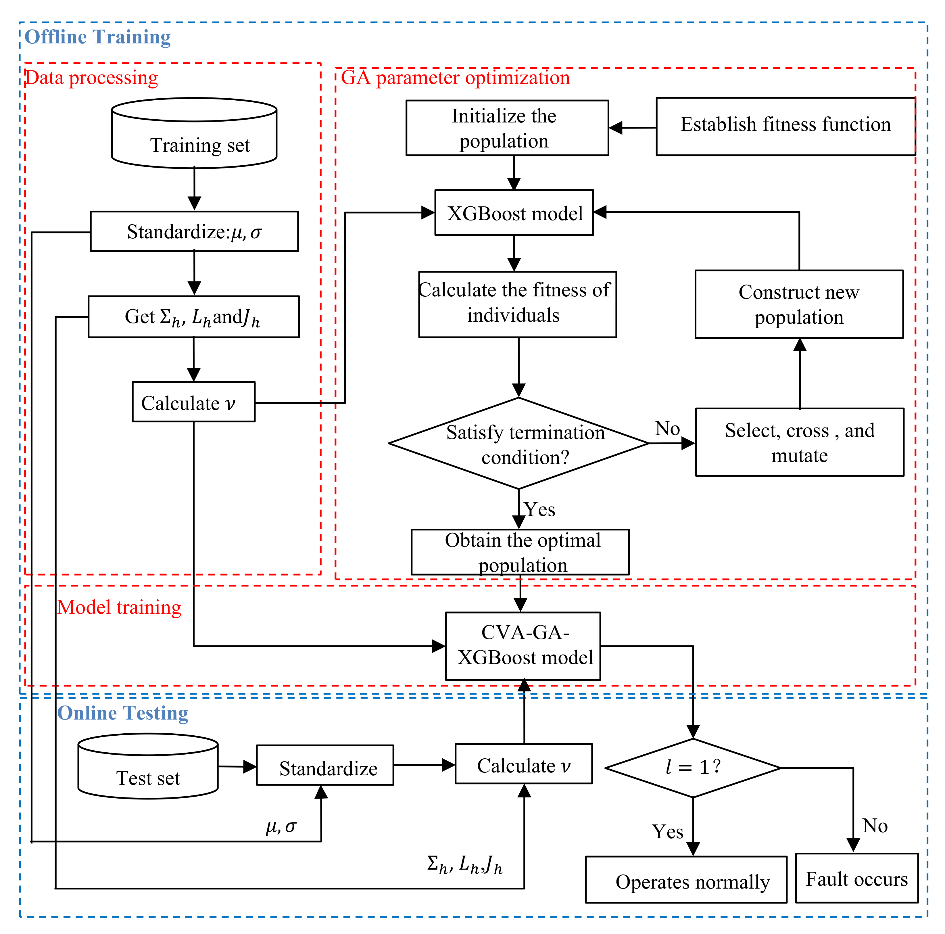
3.4. The Procedure for Fault Detection Based on CVA and GA-XGBoost

In this paper, a method that combines CVA and GA-XGBoost is used to detect the faults of the furnace negative pressure system. The flowchart of the proposed fault detection method is shown in Figure 2. In Figure 2, the purpose of offline training is to obtain the projection matrices and the optimal hyperparameters. In the offline training stage, CVA is mainly used to abstract the maximum correlation between future data and past data and construct $L_h$, $J_h$ and ${\sum }_h$. Then, the canonical residuals ${\nu }_k$ and the corresponding state labels are regarded as the inputs and outputs of XGBoost, respectively. In training the XGBoost model, the fitness function MSE is calculated using the prediction result of XGBoost and GA is used to obtain the optimal hyperparameters of XGBoost. In the online testing stage, the samples with length $p+f$ are collected for online detection. $L_h$, $J_h$ and ${\sum }_h$ are used to update the real-time canonical residuals. In Figure 2, 1 represents the normal operation and 0 represents the faulty operation. A fault can be found if the output of GA-XGBoost is 0.

3.5. The Procedure for the Proposed Fault Identification Method

The fault identification algorithm proposed in this paper is shown in Algorithm 2. The normal samples are collected to obtain the mean $\mu$ and variance $\sigma$ during the offline modeling process. In Algorithm 2, $\delta$, $\gamma$ and $\lambda$ ranges from 0 to 1 and $\delta +\gamma +\lambda =1$.

Algorithm 2. Proposed fault identification algorithm

Offline modeling:

1. Collect normal data sample x, standardize data, and obtain $\mu$ and $\sigma$.

2. Construct $p\left(k\right)$ and $f\left(k\right)$.

3. Construct $H_p$ and $H_f$.

4. Perform SVD on the scaled matrix H and obtain V, U and ∑.

5. Calculate $J=V^T{\left(\frac{1}{W-1}{H}_p{H}_p^T\right)}^{-1/2}$ and $L=U^T{\left(\frac{1}{W-1}{H}_f{H}_f^T\right)}^{-1/2}$

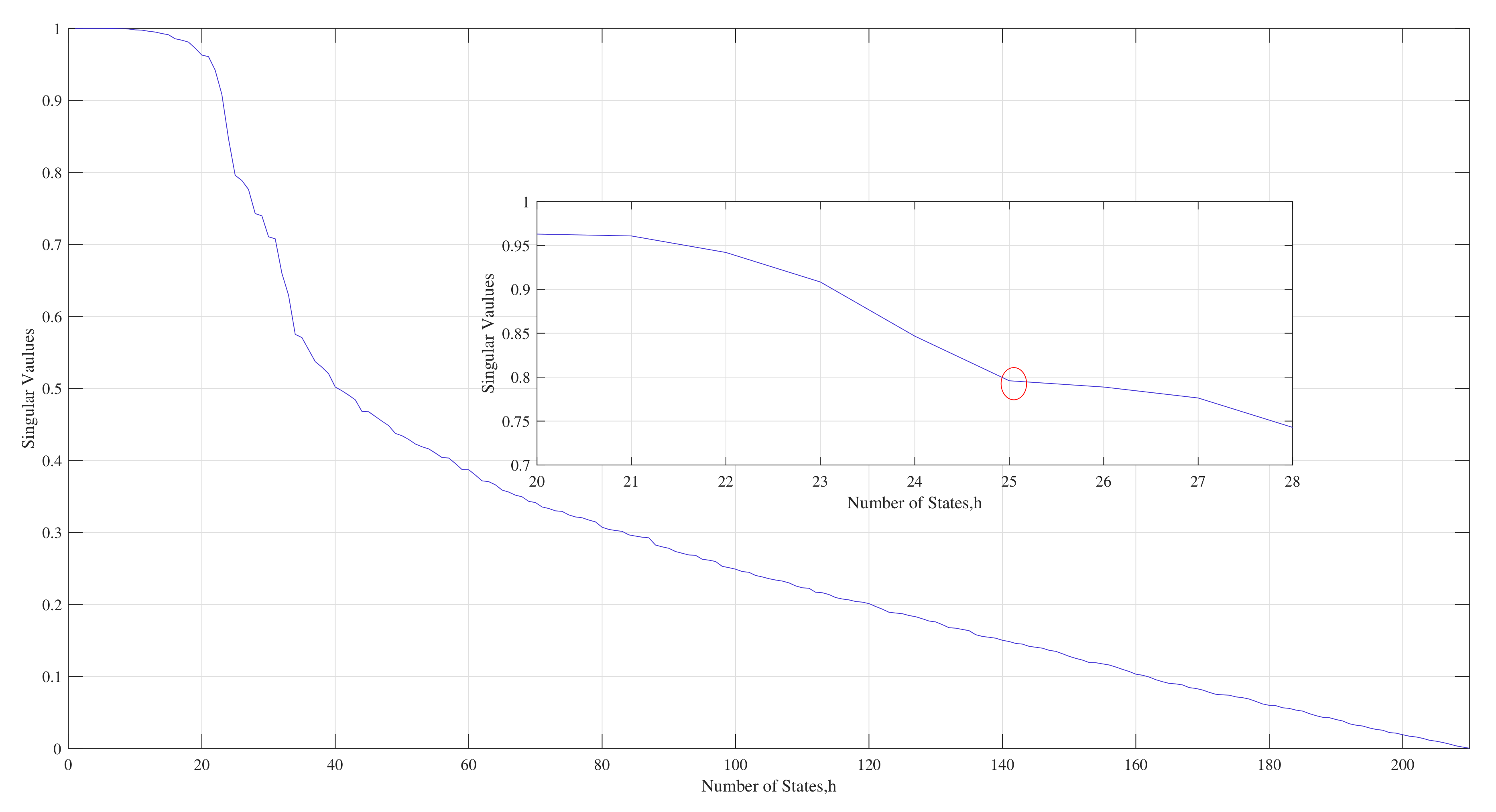
6. Determine h by the fastest descent method.

7. Construct $V_h$, $U_h$ and $F_h$.

Online identification:

1. Collect the monitoring data $x_{new}$.

2. Standardize data $\left(\mu ,\sigma \right)$.

3. Construct $p\left(k\right)$ and $f\left(k\right)$.

4. Calculate $z_k=J_{h}p\left(k\right)$, $e_k=F_{h}p\left(k\right)$

5. Calculate $T_{k,j}=z_k^T{\displaystyle {\displaystyle \sum }_{i=1}^p}\left(J_{h,\left(i-1\right)n_y+j}{p}_{\left(i-1\right)n_y+j}\left(k\right)\right)$.

6. Calculate $Q_{k,j}=e_k^T{\displaystyle {\displaystyle \sum }_{i=1}^p}\left(F_{h,\left(i-1\right)n_y+j}{p}_{\left(i-1\right)n_y+j}\left(k\right)\right)$.

7. Calculate $T_{k,j}^r={\nu }_k^T{\left(I-{\sum }_h^2\right)}^{-1}\left(\begin{array}{c}{\displaystyle {\displaystyle \sum }_{i=1}^f}{L}_{h,\left(i-1\right)n_y+j}{f}_{\left(i-1\right)n_y+j}\left(k\right)-\\ {\displaystyle {\displaystyle \sum }_{i=1}^p}{{\displaystyle \sum }}_h{J}_{h,\left(i-1\right)n_y+j}{p}_{\left(i-1\right)n_y+j}\left(k\right)\end{array}\right)$.

8. Calculate $C_{k,j}=\delta Q_{k,j}+\gamma T_{k,j}+\lambda T_{k,j}^r$.

4. Application

This example collects the true process data of furnace negative pressure control system in boiler chamber of a thermal power plant in China.

Table 1. Process variables and their descriptions.

Process Variables	Description
1	#1 exhaust fan blade opening
2	Current of exhaust fan of #1 furnace A (A)
3	#2 exhaust fan blade opening
4	Current of exhaust fan of #1 furnace B (A)
5	#1 inlet flue gas temperature of exhaust fan (°C)
6	#1 flue gas pressure at the outlet of dust collector (Pa)
7	#2 inlet flue gas temperature of exhaust fan (°C)
8	#2 flue gas pressure at the outlet of dust collector (Pa)
9	#1 blower blade opening
10	Current of blower of #1 furnace A (A)
11	#2 blower blade opening
12	Current of blower of #1 furnace B (A)
13	#1 furnace A primary fan current (A)
14	#1 furnace B primary fan current (A)
15	Side A steam header pressure (MPa)
16	Side A steam header temperature (°C)
17	Compensated blower outlet air volume (t/h)
18	Oxygen content of tail flue gas (%)
19	Furnace negative pressure (Pa)
20	Generator active power (MW)
21	main steam flow (t/h)

presents 21 process variables (PVs) closely related to the working condition of the furnace negative pressure control system.

In this example, a fault occurs in the exhaust fan of # 1 furnace A, in which the exhaust motor blade was jammed. Figure 3 shows the diagram of the base cracking of the exhaust fan blade actuator. When the moving blade of the exhaust fan of #1 furnace A is jammed, the output of the #1 exhaust fan will change and the #2 exhaust fan will track the set point of the furnace negative pressure the automatic state to adjust the furnace negative pressure to be stable. Therefore, the amount of flue gas passing through the #1 and #2 exhaust fan will change, which results in a change in the temperature of the flue gas at the #1 and #2 exhaust fan inlet. Although it has been adjusted by #2 induced draft fan, there is still a certain gap comparing with normal operation. In order to maintain the balance of the pressure in the furnace, it is necessary to adjust the output of the blower, which causes the change of the current of the blower of the #1 furnace A.

In training the CVA model, 4000 normal samples are considered. First, autocorrelation analysis is performed on 4000 normal samples to obtain the number of time lags in the past and future data (p and f). In this case, the ten number of lag is the maximum, after which the autocorrelation does not change significantly within the 5% confidence interval. Therefore, both p and f are set to 10. Figure 4 shows the singular values of the Hankel matrix H. The number of h states in the CVA model is determined according to the trend of the singular values of H. In this paper, the fastest descent method is adopted to decide the proper h and h is considered to be the “critical” point in the singular value curve. According to the point inside the red circle in Figure 4, $h=25$.

To train the fault detection model, 4000 normal samples and 2000 fault samples are collected to compose the training set. Then, the model residuals $v_k$ of the training set are calculated based on p, f and h obtained during CVA training. The $v_k$ is taken as the input of GA-XGBoost and its corresponding label as the output of GA-XGBoost. The GA-XGBoost algorithm is used to build the fault detection model. If the output of GA-XGBoost model is 1, it means that the furnace operates normally. If the output of GA-XGBoost model is 0, it means that a fault occurs. After constructing the fault detection model, 4880 samples are used to online detect the faults. In this paper, the detection rate ${\mathrm{I}}_{DR}$ and the false positive rate ${\mathrm{I}}_{FAR}$ are used to measure the performance of the proposed method. The definitions of ${\mathrm{I}}_{DR}$ and ${\mathrm{I}}_{FAR}$ are given as:

$$\left\{\begin{array}{c}{\mathrm{I}}_{DR}=\frac{{\mathrm{N}}_1}{{\mathrm{N}}_{abnormal}}\times 100\%\\ {\mathrm{I}}_{FAR}=\frac{{\mathrm{N}}_2}{{\mathrm{N}}_{normal}}\times 100\%\end{array}\right.$$

(20)

where ${\mathrm{N}}_{abnormal}$ represents the number of the true fault, ${\mathrm{N}}_1$ represents the number of fault detected, ${\mathrm{N}}_{normal}$ represents the number of the true normal samples, and ${\mathrm{N}}_2$ represents the number of the normal samples diagnosed as faults. A higher $I_{DR}$ combining with a lower $I_{FAR}$ indicates the better performance of the proposed method.

The proposed method is compared with CVA, PCA-SVM and PLS-SVM. Figure 5 presents the fault detection result of CVA, with Figure 5a for CVA-$T_k$, Figure 5b for CVA-$Q_k$ and Figure 5c for CVA-$T_k^r$. The control limits of the three monitoring indicators of CVA are obtained by the kernel density estimation method. In Figure 5a,b, the indicators CVA-$T_k$ and CVA-$Q_k$ in the monitoring phase always exceed their control limits and all of the normal samples are judged to be abnormal. In Figure 5c, CVA-$T_k^r$ are larger than the control limit from the 2752nd sample, and 1249 normal samples are mistakenly diagnosed as malfunctions. This result indicates the two traditional CVA indicators and the newly defined indicator CVA-$T_k^r$ are ineffective to discover the abnormal events of the furnace negative pressure systems. Figure 6 presents the fault detection result of PCA-SVM, from which about 200 faulty samples are judged to be normal. Thus, the detection rate of PCA-SVM is much low. Figure 7 presents the fault detection result of PLS-SVM. All of the faulty samples are judged to be normal, indicating that the PLS-SVM method is invalid for this example. Figure 8 exhibits the fault detection result of the proposed method. In Figure 8, only 12 normal samples are misdiagnosed as malfunctions and only four faulty samples are judged to be normal. As seen from Figure 6, Figure 7 and Figure 8, the number of fault samples correctly detected by the proposed method is much larger than those by PCA-SVM and PLS-SVM. As seen from Figure 5 and Figure 8, the number of the normal samples incorrectly detected by the proposed method is much smaller than that by CVA. Therefore, compared with CVA, PCA-SVM and PLS-SVM, the proposed method is more effective to discover the abnormal events of the furnace negative pressure system.

Table 2. The detection rate, false alarm rate and detection time of the four methods.

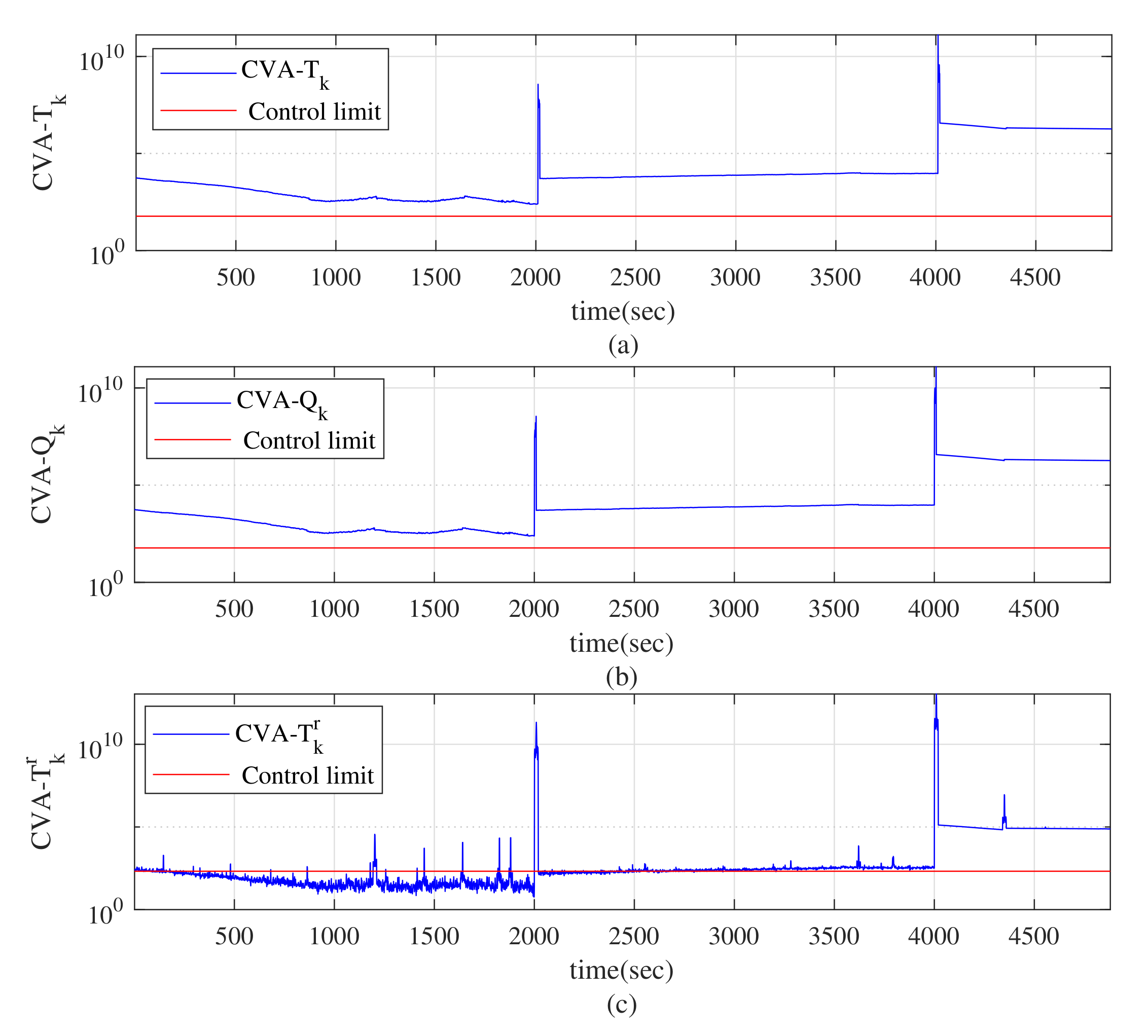
Method	I${}_{\mathit{DR}}$	I${}_{\mathit{FAR}}$	Detection Time
CVA-$T_k$	1	1	3.330 s
CVA-$Q_k$	1	1	3.307 s
CVA-$T_k^r$	1	0.4203	3.561 s
PCA-SVM	0.3148	0	7.304 s
PLS-SVM	0	0	8.403 s
CVA-GA-XGBoost	0.9955	0.0030	3.481 s

gives the detection rate, the false positive rate and the detection time of the four methods. As shown in Table 2, the ${\mathrm{I}}_{FAR}$ of CVA-$T_k$ and CVA-$Q_k$ are 1, indicating that CVA-$T_k$ and CVA-$Q_k$ are ineffective to distinguish the normal samples from the faulty samples. The ${\mathrm{I}}_{DR}$ of the PLS-SVM method is 0, indicating that PLS-SVM is unable to find the abnormal events. The ${\mathrm{I}}_{FAR}$ of the proposed method is 0.0030, which is much smaller than that of CVA-$T_k$, and the ${\mathrm{I}}_{DR}$ of the proposed method is 0.9955, which is only 0.0045 smaller than that of CVA-$T_k^r$. This result indicates that the false alarm rate of the proposed method is much smaller than that of CVA. The ${\mathrm{I}}_{DR}$ of the proposed method is three times larger than that of PCA-SVM, and the ${\mathrm{I}}_{FAR}$ of the proposed method is almost equal to that of PCA-SVM. This result indicates that the detection rate of the proposed method is much larger than that of PCA-SVM. In Table 2, the detection time of the proposed method is 3.481 s, which is 0.0163 s less than that of CVA-$T_k^r$. The detection times of PCA-SVM and PLS-SVM are 7.304 s and 8.403 s, respectively. However, since the canonical residuals constructed by CVA are used to obtain the proposed fault detection model, the detection time of the proposed method is 0.151 s more than that of CVA-$T_k$ and CVA-$Q_k$. This result means that the detection time of the proposed method is much less than that of PCA-SVM and PLS-SVM while it is a little more than that of CVA-$T_k$ and CVA-$Q_k$. Therefore, the proposed method is the most effective than the other three methods in detecting the faults of the furnace negative pressure system for the real thermal power plants.

After detecting the fault, the faulty variables need to be identified. The fault identification results based on state space and canonical residual space are shown in Figure 9 and Figure 10, respectively. In Figure 10, #2 inlet flue gas temperature of exhaust fan (PV7) and current of blower of #1 furnace A (PV10) are identified in several samples. However, no PVs are identified in the subsequent contribution plots. This result suggests that the variable contribution of state space and that of canonical residual space are unable to identify the faulty variable. The fault identification result of the proposed method is shown in Figure 11. For the reconstructed variable contribution of this example, the weights on the residual space, the state space and the space residual space are 0.6, 0.2 and 0.2, respectively. As seen from Figure 11, there are four PVs are identified as faulty variables, such as the current of exhaust fan of #1 furnace A (PV2), #1 inlet flue gas temperature of exhaust fan (PV5), PV7 and PV10. Besides, the contributions of the four PVs always exist. Figure 12 presents the online PV2, PV5, PV7 and PV10. As shown in Figure 12, there is a sharp increase in PV2 and PV5, and there is a sharp decrease in PV7 and PV10 when the fault occurs. It can also be seen from Figure 12 that the changes in PV2 and PV7 are much more significant than those in PV5 and PV10, meaning that the current fault has a more significant effect on PV2 and PV7 than that on PV5 and PV10. Figure 11 clearly shows that the contributions of PV2 and PV7 are much greater than those of PV5 and PV10. This result demonstrates that the proposed method can accurately identify the variables related to the fault. Therefore, the fault identification method based on reconstructed variable contribution is effective for the furnace negative pressure system of the thermal power plant.

5. Conclusions

In this paper, a novel fault detection and identification method based on CVA and GA-XGBoost is proposed for the furnace negative pressure system of a boiler. The CVA method processes the original data to remove noise in the data and constructs the canonical residual vector that quantifies the difference between the future vector and the past vector. The fault detection model based on GA-XGBoost is built using the canonical residuals of the training set. The seven key hyperparameters of XGBoost, including Learning_rate, n_estimators, max_depth, min_child_weight, subsample, colsample_bytree and gamma, are optimized by GA to improve the prediction accuracy. A novel fault identification method based on reconstructed contribution graph is proposed, which can simultaneously capture the abnormal information contained in the state space, residual space and canonical residual space, and the ability of the method can be improved by changing the weights. The furnace negative pressure system of a boiler in a thermal power plant is used to demonstrate the effectiveness of the proposed fault detection and identification method. The ${\mathrm{I}}_{DR}$ of the proposed method is greater than 0.99, which is significantly larger than that of PCA-SVM and PLS-SVM, and the ${\mathrm{I}}_{FAR}$ is lower than 0.01, which is significantly smaller than that of CVA. The proposed fault identification method identifies the variables related to the fault correctly. This result demonstrates that the method proposed in this paper is superior to CVA, PCA-SVM and PLS-SVM.

References

- Khan, F.; Haddara, M.; Khalifa, M. Risk-based inspection and maintenance (RBIM) of power plants Thermal Power. In Plant Performance Analysis; Springer: London, UK, 2012; pp. 249–279. [Google Scholar]
- He, K.X.; Wang, T.; Zhang, F.K.; Jin, X. Anomaly detection and early warning via a novel multiblock-based method with applications to thermal power plants. Measurement 2022, 193, 110979. [Google Scholar] [CrossRef]
- Yu, J.; Jang, J.; Yoo, J.; Park, J.H.; Kim, S. A fault isolation method via classification and regression tree-based variable ranking for drum-type steam boiler in thermal power plant. Energies 2018, 11, 1142. [Google Scholar] [CrossRef]
- Shi, Y.H.; Wang, J.C.; Liu, Z.F. On-line monitoring of ash fouling and soot-blowing optimization for convective heat exchanger in coal-fired power plant boiler. Appl. Therm. Eng. 2015, 78, 39–50. [Google Scholar] [CrossRef]
- Agrawal, V.; Panigrahi, B.K.; Subbarao, P.M.V. Review of control and fault diagnosis methods applied to coal mills. J. Process. Control 2015, 32, 138–153. [Google Scholar] [CrossRef]
- Peng, X.; Ding, S.X.; Du, W.L.; Zhong, W.M.; Qian, F. Distributed process monitoring based on canonical correlation analysis with partly-connected topology. Control Eng. Pract. 2020, 101, 104500. [Google Scholar] [CrossRef]
- Forootan, M.M.; Larki, I.; Zahedi, R.; Ahmadi, A. Machine Learning and Deep Learning in Energy Systems: A Review. Sustainability 2022, 14, 4832. [Google Scholar] [CrossRef]
- Yu, K.J.; While, L.; Reynolds, M.; Liang, J.J.; Zhao, L.; Wang, Z.L. Multiobjective optimization of ethylene cracking furnace system using self-adaptive multiobjective teaching-learning-based optimization. Energy 2018, 148, 469–481. [Google Scholar] [CrossRef]
- Jagtap, H.P.; Bewoor, A.K. Use of analytic hierarchy process methodology for criticality analysis of thermal power plant equipments. Mater. Today Proc. 2017, 4, 1927–1936. [Google Scholar] [CrossRef]
- Li, W.; Peng, M.J.; Wang, Q.Z. False alarm reducing in PCA method for sensor fault detection in a nuclear power plant. Ann. Nucl. Energy 2018, 118, 131–139. [Google Scholar] [CrossRef]
- Li, W.; Peng, M.J.; Wang, Q.Z. Improved PCA method for sensor fault detection and isolation in a nuclear power plant. Nucl. Eng. Technol. 2019, 51, 146–154. [Google Scholar] [CrossRef]
- Qin, Y.H.; Lou, Z.J.; Wang, Y.Q.; Lu, S.; Sun, P. An analytical partial least squares method for process monitoring. Control Eng. Pract. 2022, 124, 105182. [Google Scholar] [CrossRef]
- Pilario, K.E.S.; Cao, Y. Canonical variate dissimilarity analysis for process incipient fault detection. IEEE Trans. Ind. Inform. 2018, 14, 5308–5315. [Google Scholar] [CrossRef]
- Chiang, L.H.; Kotanchek, M.E.; Kordon, A.K. Fault diagnosis based on Fisher discriminant analysis and support vector machines. Comput. Chem. Eng. 2004, 28, 1389–1401. [Google Scholar] [CrossRef]
- Jiang, Q.C.; Yan, X.F.; Huang, B. Review and perspectives of data-driven distributed monitoring for industrial plant-wide processes. Ind. Eng. Chem. Res. 2019, 58, 12899–12912. [Google Scholar] [CrossRef]
- Odgaard, P.F.; Bao, L.; Jorgensen, S.B. Observer and Data-Driven-Model-Based Fault Detection in Power Plant Coal Mills. IEEE Trans. Energy Convers. 2008, 23, 659–668. [Google Scholar] [CrossRef]
- Yu, Y.; Peng, M.; Wang, H.; Ma, Z. Multivariate Alarm Threshold Design Based on PCA. In International Congress and Workshop on Industrial AI; Springer: Cham, Switzerland, 2022. [Google Scholar] [CrossRef]
- Liu, G.J.; Gu, H.X.; Shen, X.C.; You, D.D. Bayesian long short-term memory model for fault early warning of nuclear power turbine. IEEE Access 2020, 8, 50801–50813. [Google Scholar] [CrossRef]
- Ajami, A.; Daneshvar, M. Data driven approach for fault detection and diagnosis of turbine in thermal power plant using Independent Component Analysis (ICA). Int. J. Electr. Power Energy Syst. 2012, 43, 728–735. [Google Scholar] [CrossRef]
- Li, D.; Hu, G.Q.; Spanos, C.J. A data-driven strategy for detection and diagnosis of building chiller faults using linear discriminant analysis. Energy Build. 2016, 128, 519–529. [Google Scholar] [CrossRef]
- Xia, Y.; Ding, Q.; Jing, N.; Tang, Y.; Jiang, A.; Jiangzhou, S. An enhanced fault detection method for centrifugal chillers using kernel density estimation based kernel entropy component analysis. Int. J. Refrig. 2021, 129, 290–300. [Google Scholar] [CrossRef]
- Kourti, T.; MacGregor, J.F. Multivariate SPC methods for process and product monitoring. J. Qual. Technol. 1996, 28, 409–428. [Google Scholar] [CrossRef]
- Alcala, C.F.; Qin, S.J. Reconstruction-based contribution for process monitoring. Automatica 2009, 45, 1593–1600. [Google Scholar] [CrossRef]
- Liu, J.L. Fault diagnosis using contribution plots without smearing effect on non-faulty variables. J. Process. Control. 2012, 22, 1609–1623. [Google Scholar] [CrossRef]
- Liu, J.L.; Chen, D.S. Fault isolation using modified contribution plots. Comput. Chem. Eng. 2014, 61, 9–19. [Google Scholar] [CrossRef]
- Tan, R.M.; Cao, Y. Deviation contribution plots of multivariate statistics. IEEE Trans. Ind. Inform. 2018, 15, 833–841. [Google Scholar] [CrossRef]
- Zhu, X.X.; Braatz, R.D. Two-dimensional contribution map for fault identification [focus on education]. IEEE Control Syst. Mag. 2014, 34, 72–77. [Google Scholar]
- Jiang, B.B.; Huang, D.X.; Zhu, X.X.; Yang, F.; Braatz, R.D. Canonical variate analysis-based contributions for fault identification. J. Process. Control 2015, 26, 17–25. [Google Scholar] [CrossRef]
- Li, X.C.; Yang, X.Y.; Yang, Y.J.; Bennett, L.; Collop, A.; Mba, D. Canonical variate residuals-based contribution map for slowly evolving faults. J. Process. Control 2019, 76, 87–97. [Google Scholar] [CrossRef]
- Rangel-Martinez, D.; Nigam, K.D.P.; Ricardez-Sandoval, L.A. Machine learning on sustainable energy: A review and outlook on renewable energy systems, catalysis, smart grid and energy storage. Chem. Eng. Res. Des. 2021, 174, 414–441. [Google Scholar] [CrossRef]
- Pirdashti, M.; Curteanu, S.; Kamangar, M.H.; Hassim, M.H.; Khatami, M.A. Artificial neural networks: Applications in chemical engineering. Rev. Chem. Eng. 2013, 29, 205–239. [Google Scholar] [CrossRef]
- Mahadevan, S.; Shah, S.L. Fault detection and diagnosis in process data using one-class support vector machines. J. Process Control 2009, 19, 1627–1639. [Google Scholar] [CrossRef]
- Chen, K.Y.; Chen, L.S.; Chen, M.C.; Lee, C.L. Using SVM based method for equipment fault detection in a thermal power plant. Comput. Ind. 2011, 62, 42–50. [Google Scholar] [CrossRef]
- Moradi, M.; Chaibakhsh, A.; Ramezani, A. An intelligent hybrid technique for fault detection and condition monitoring of a thermal power plant. Appl. Math. Model. 2018, 60, 34–47. [Google Scholar] [CrossRef]
- Deb, C.; Zhang, F.; Yang, J.J.; Lee, S.E.; Shah, K.W. A review on time series forecasting techniques for building energy consumption. Renew. Sustain. Energy Rev. 2017, 74, 902–924. [Google Scholar] [CrossRef]
- Wang, H.; Peng, M.J.; Hines, J.W.; Zheng, G.Y.; Liu, Y.K.; Upadhyaya, B.R. A hybrid fault diagnosis methodology with support vector machine and improved particle swarm optimization for nuclear power plants. ISA Trans. 2019, 95, 358–371. [Google Scholar] [CrossRef]
- Wang, Z.Y.; Yao, L.G.; Cai, Y.W.; Zhang, J. Mahalanobis semi-supervised mapping and beetle antennae search based support vector machine for wind turbine rolling bearings fault diagnosis. Renew. Energy 2020, 155, 1312–1327. [Google Scholar] [CrossRef]
- Chen, T.Q.; Guestrin, C. XGBoost: A scalable tree boosting system. In Proceedings of the 22nd ACM SIGKDD International Conference on Knowledge Discovery and Data Mining, San Francisco, CA, USA, 13–17 August 2016; pp. 785–794. [Google Scholar]
- Xiang, C.; Ren, Z.J.; Shi, P.F.; Zhao, H.G. Data-Driven Fault Diagnosis for Rolling Bearing Based on DIT-FFT and XGBoost. Complexity 2021, 2021, 4941966. [Google Scholar] [CrossRef]
- Holland, J.H. Adaptation in Natural and Artificial Systems: An Introductory Analysis with Applications to Biology; University of Michigan Press: Ann Arbor, MI, USA, 1975. [Google Scholar]
- Feng, Z.W.; Guan, N.; Lv, M.S.; Liu, W.C.; Deng, Q.X.; Liu, X.; Yi, W. Efficient drone hijacking detection using two-step GA-XGBoost. J. Syst. Archit. 2020, 103, 101694. [Google Scholar] [CrossRef]
- Zhang, D.H.; Qian, L.Y.; Mao, B.J.; Huang, C.; Si, Y.L. A Data-Driven Design for Fault Detection of Wind Turbines Using Random Forests and XGBoost. IEEE Access 2018, 6, 21020–21031. [Google Scholar] [CrossRef]
- Fitriah, N.; Wijaya, S.K.; Fanany, M.I. EEG channels reduction using PCA to increase XGBoost’s accuracy for stroke detection. AIP Conf. Proc. 2017, 1862, 030128. [Google Scholar]