Abstract
The conventional fracture in shale hydraulic fracturing belongs to the type-I fracture, and the size of the fracture process zone (FPZ) is an important index to measure the fracability of rock mass. This index is also one of the feasible entry points to study the complexity of the fracture network. In order to visually observe the type-I FPZ at the tip of shale fractures, and to study the relationship between the mechanical properties, the shape and size of the FPZ, and the bedding structure, Notched Semi-Circular Bend (NSCB) tests were conducted with three typical fracture direction-bedding orientations (splitter, arrester, divider). The digital image correlation (DIC) method was used to realize the intuitive observation of the real fracture process and the FPZ near the fracture tip. The test found that the FPZ of shale is narrow and long as a whole and is “flame-like”. The height-to-length ratio of the FPZ at the fracture tip determines whether bending and deflection happen between the new fracture and the prefabricated cracks when the fracture occurs. Most of the specimens often appear in the FPZ with a beaded high shear strain zone before the fracture, which is caused by the oblique communication of micro-cracks in the FPZ before the fracture. The appearance of a beaded zone of high shear strain indicates that macroscopic fracture is imminent. The research results can be used for the design of disaster early warning and prevention programs.
1. Introduction
Reservoir shale is the carrier of shale gas and also the matrix for the formation of fracturing networks. Studying the characteristics of reservoir shale is the basis for exploring the complicated mechanism of the fracturing network. Among the many characteristics of reservoir shale, researchers pay more attention to these aspects, including the anisotropy of basic mechanical indicators, fracture toughness, brittleness, fracability, etc. The continuous changes of the depositional environment and sediment composition over time during the shale deposition process result in the unique lamination structure of shale. The composite material formed by the lamination of rock-like materials, its elastic modulus, Poisson’s ratio, compressive and tensile strength, wave speed, electromagnetic response parameters, and other characteristic parameters will change with the difference between the measurement direction and the angle between the sedimentary layers. Thus, it is difficult to use a single numerical value to characterize a certain mechanical property of the rock as a whole, and this type of anisotropy is also called transverse isotropy [1]. Guo et al. [2] pointed out that the development of shale fractures and irregularly filled clay minerals are the main reasons for shale anisotropy.
Josh et al. [3] analyzed the microstructure and anisotropic characteristics of shale by CT and electron microscope scanning techniques and pointed out that this anisotropic characteristic is mainly caused by the clay mineral filling and fracture development of shale. Bayuk et al. [4] believed that attention should be paid to the influence of anisotropy caused by the development of fractures and the irregular filling of clay minerals on the microseismic monitoring signals. Banik [5] studied the anisotropy of shale wave velocity and its causes and pointed out that the wave velocity in the vertical deposition direction is larger than that in the parallel deposition direction, and the main reason for this is that there are gaps and clay filling in the sedimentary layer. Lekhnitskii [6] established the theoretical foundation of anisotropic rock mechanics by solving the elastic solutions of differential equations of anisotropic media with the classical theory of elasticity of continuum media. Wardle and Gerrard [7] introduced the concept of equivalent anisotropy and its suitability for layered media (such as shale materials). Salamon [8] proposed an equivalent model of layered medium and established a mechanical structure model of layered rock mass by simplifying the rock material of the actual complex structure into a homogeneous transversely isotropic material, and then they used five independent parameters to mark the transversely isotropic characteristics, with the isotropy along the deposited layer and the anisotropy along the vertical deposited layer. Based on this model, the authors further simplified the layered rock mass as a layered composition of plate-like uniform elastomers, and the mechanical properties of each layer of material correspond to different elastic parameters. Many researchers carried out uniaxial compressive tests and Brazilian splitting tests of plate-like rocks (shale, schist, mudstone) and summarized the change law of compressive strength, tensile strength, elastic modulus, and Poisson’s ratio [9,10,11,12]. Pomeroy et al. [13] conducted triaxial compression tests on hard coal rock and diatomite rock, respectively, then analyzed the changes of mechanical parameters with the increase of confining pressure. Wang et al. [14] conducted uniaxial compression tests and pseudo-triaxial stress difference compression tests on several types of schist and analyzed the axial and radial deformation of various types of specimens with the change of the inclination angle of the weak plane and different confining pressure conditions. Shi et al. [15] evaluated the applicability of different test methods for testing the mutual orthogonal mechanical parameters of rock in three directions by performing uniaxial compression, Brazilian splitting, and ring restraint experiments on anisotropic rocks.
Fracture toughness is a characteristic index used to measure the difficulty of crack propagation, and it is an important parameter that affects the hydraulic pressure of fracture initiation. The fracture toughness of shale exhibits an obvious difference in the different sedimentary layers. Ke [16] measured the fracture toughness of shale using the three-point bending round bar method (CB) recommended by the International Society of Rock Mechanics. Many researchers carried out type-I fracture toughness anisotropy and composition tests and pointed out that the fracture toughness of Anvil Points oil shale is not only related to the bedding angle, but also to the content of organic matter in the shale [17,18,19]. Timoshenko et al. [20] believed that the material showed a sudden disappearance of ductility at the end of the plastic zone in the latter part of the stress-strain curve, and they indicated that the material showed brittleness in this state. The Poisson-Young method proposed by Rickman at the SPE conference in 2008 considers that rock brittleness is positively related to Young’s elastic modulus and negatively related to Poisson’s ratio [21]. It is easy to obtain a continuous brittleness index (also known as sonic brittleness index) by logging continuously, and this method is widely used in the field of oil and gas engineering.
Regarding the mechanism of the initiation and propagation of hydraulic fractures, the current mainstream view is that when the tensile stress of the weak structure plane of the rock in the area of hydraulic pressure exceeds its tensile strength, the fractured micro-cracks penetrate each other to form tensile fractures connected with the perforation [22]. When the fracturing fluid fills the fracture, the stress intensity factor of the fracture tip increases with the increase of the water pressure in the fracture. When the fracture toughness of the rock at the fracture tip exceeds the fracture toughness, the hydraulic fracture expands [22,23]. However, there exist many factors affecting the local tensile stress and fracture stress intensity factor near the tip, and the influencing process is complicated; the basic hydraulic fracture mechanism cannot be directly used to guide the practice of hydraulic fracturing engineering.
Therefore, this paper mainly discusses the fracture mechanism and combined the DIC method to carry out shale fracture tests. Based on the data obtained from the test results, such as deformation field and strain field, the FPZ of various shale specimens under different bedding orientation loading was observed, and the characteristics of the rock fracture process and its rupture mechanism were analyzed in further steps.
2. FPZ Theory
The traditional theory of the rock fracture process proposed by Atkinson et al. [24] holds that, when loading a cracked specimen with materials such as rock or ceramics as the medium, the fracture process should be as shown in Figure 1. From stage A to stage E in Figure 1, as the stress continues to increase, micro-cracks develop and finally form macro-cracks and expand forward. Stage A: Initially due to stress concentration, a small number of microscopic cracks isolated from each other are formed at the crack tip. Stage B: As the load continues to increase, the high stress range near the crack tip expands and companying the number of microcracks increases, while the microcracks are still relatively isolated; thus, the overall structure maintains linear elastic properties. Stage C: The microcracks continue to increase, some microcracks even begin to affect each other, and the end region of the cracks begins to exhibit nonlinear properties. Stage D: In the fully developed process region, the microcracks are connected with each other, leading to macro crack propagation. Stage E: With the movement of the pre-macro crack process region, the macro crack further expands. The description of stage E in traditional fracture process theory implies that the development of the process zone precedes the expansion of macroscopic fractures, and the macroscopic fractures do not extend beyond the current process zone.
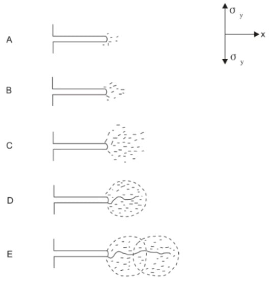
Figure 1.
FPZ development and its effect on macroscopic crack propagation [24].
Atkinson [24] called the region with nonlinear characteristics near the crack tip the FPZ due to the accumulation of micro-cracks, and some scholars also called it the damage zone, plastic zone, and nonlinear zone. The micro-crack cluster in the process zone is the damage cloud of the tip medium under a high stress state, and the expansion of the macro-crack is accompanied by the movement of the process zone and the damage cloud in the process zone. Atkinson also pointed out that the term “process zone”, which is generally used to express full-process tracing, includes all the nonlinear behavior in the region of the crack tip, but, for rocks, it initially appears as an expansion zone characterized by the formation of numerous micro-cracks. A large number of brittle rock fracture process observations show that such microcracks can appear at a considerable distance from the macro crack tip, which is comparable to the scale of commonly used specimens; that is, the real process zone size can be the same order of magnitude as the specimen size.
Irwin [25] gave the polar coordinate Mises yield formula under the critical condition of plastic failure as shown in Equation (1), and, based on this, the contour and range of the crack tip process region were given as shown in Figure 2.

Figure 2.
The shape and size of the process zone near the crack tip calculated theoretically [25].
In particular, when θ = 0, the diameter of the process zone in the direction of the crack propagation is obtained:
Irwin also made a simple correction to the stress intensity factor K of brittle rock and replaced the original crack length with the equivalent crack length, c = a + r0, so that the linear elastic fracture criterion after the correction can be applied to rock materials.
It is worth noting that Irwin’s theoretical calculation does not consider the influence of the stress relaxation effect in the process zone. This effect can reduce the degree of stress concentration in the process zone so that the maximum true stress in the process zone is lower than the theoretically calculated maximum stress. The area range increases, even if the real process zone size r0 is larger than the theoretically calculated value in Equation (2), specifically as is shown in Figure 3.
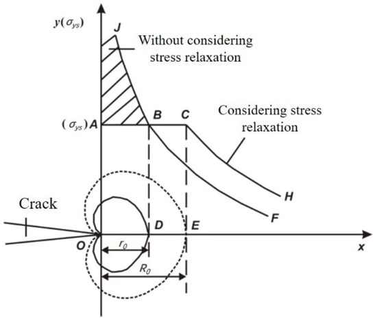
Figure 3.
The effect of stress relaxation on fracture process zone size [25].
At present, different opinions exist on the specific calculation formula of the size for the rock FPZ, but the opinion with a high degree of acceptance holds that no matter whether the process zone expands due to stress relaxation or not, its size range diameter is positively correlated with the square of the bracket in Equation (2), namely:
The size of the process zone is an important index to measure the rock fracability, and it is also one of the feasible entry points used to study the complexity of the fracture network.
The strain field at the crack tip can be obtained using the DIC method. The premise of obtaining the process zone at the crack tip according to the strain field is that there must be a criterion for measuring which areas near the crack tip enter the process zone and which areas are outside the process zone, that is, the damage criterion. At present, the academic community has not formed a unified consensus on the criterion for judging the FPZ (also known as the damage zone) at the crack tip, but it is generally believed that the process zone is nominally in the yield stage; thus, the process zone is also called the nominal plastic zone. At present, the most widely used is the maximum tensile stress criterion based on the first strength theory, as shown in Formula (4):
Among them, σ1 is the maximum tensile stress, and σt is the tensile strength of the material. This criterion considers that, in the area near the crack tip, the area where the maximum tensile stress reaches or exceeds the tensile strength of the rock has actually suffered a certain degree of damage, and thus it is located in the process zone; the area where the maximum tensile stress is less than the tensile strength, no damage has occurred, and thus it is outside the process zone.
However, shale is an anisotropic material; it is difficult to convert its tensile stress from the strain field obtained by the DIC method, but its maximum tensile strain can be obtained according to its strain field distribution. Then, the maximum tensile strain criterion based on the second strength theory is used. Therefore, it is very convenient to judge whether the crack tip area enters the process zone. Here, Equation (5) can also be used as the criterion for delineating the crack process zone:
where ε1 is the maximum tensile strain, and εtc is the material critical tensile strain. This criterion considers that, in the region near the crack tip, the region where the maximum tensile strain reaches or exceeds the critical tensile strain εtc has actually undergone a certain degree of damage (microscopic cracks are generated inside) or has entered a nonlinear stage; thus, it can be considered that it is located within the process zone. The area where the maximum tensile strain ε1 is less than the material critical tensile strain εtc is slightly damaged; thus, it can be considered to be outside the process zone.
Critical tensile strain is a material mechanical property similar to tensile strength; considering that shale is an anisotropic material, the critical tensile strain εtc will change when the loading direction or crack propagation direction has a different azimuthal relationship with the bedding. Therefore, in order to analyze the change of the FPZ at the crack tip, it is necessary to study the anisotropy of the critical tensile strain εtc of shale. By carrying out compression tests of three typical loading methods on unfractured shale specimens, the surface strain field before failure of the specimens was obtained by means of DIC, and then the critical tensile strain of the shale specimen when the loading direction and bedding were in three typical orientations was obtained, along with the changes in εtc and other key parameters. According to the results of the fracture test, the intuitive distribution map of the FPZ at the crack tip of the specimen was obtained. Based on these data, three modes of εtc corresponding to the three loading-direction bedding orientations were obtained to determine the type-I FPZ of the sample.
3. Sample Preparation and Instrumentation
3.1. Sample Processing
In this paper, the NSCB specimen with no change of shape or structure in the thickness direction, recommended by International Society of Rock Mechanics (ISRM), was used. The geometric configuration is shown in Figure 4. The recommended value range and the design value selected in this experiment are shown in Table 1. Considering the transverse isotropy of shale, different fracture characteristics will be presented when the cracking direction and the bedding orientation are different. Therefore, three typical cracking direction-bedding orientations (splitter, arrester, and divider) were processed in this paper (as shown in Figure 5), and then the deformation near the crack tip before the fracture was observed by DIC. Accordingly, the FPZ near the crack tip was delineated. For comparison, Figure 5 also shows the non-cracked cuboid specimens with a length of 50 mm, a width of 30 mm, and a thickness of 10 mm with three cracking-direction bedding orientations.
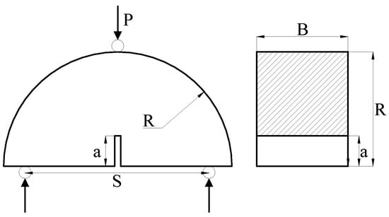
Figure 4.
Specimen geometry and ligament surface.

Table 1.
NSCB specimen geometry specifications.
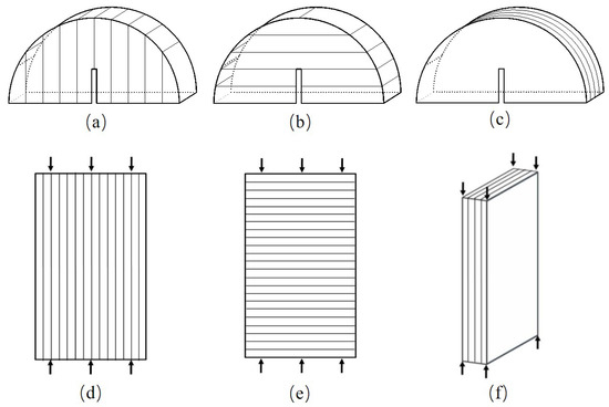
Figure 5.
Three modes of shale fracture specimens and corresponding non-cracked specimens: (a) splitter-mode fracture specimen, (b) arrester-mode fracture specimen, (c) divider-mode fracture specimen, (d) splitter-mode non-cracked specimen, (e) arrester-mode non-cracked specimen, (f) divider-mode non-cracked specimen.
A cylinder with a 75 mm diameter was drilled parallel and perpendicular to the shale bedding and cut into thin discs with a thickness of 30 mm, and then the NSCB specimens were prepared by a diamond wire cutting machine as shown in Figure 6.
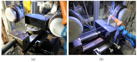
Figure 6.
NSCB specimens prepared by a diamond wire cutting machine: (a) semicircle cut by a diamond wire cutting machine; (b) slit by diamond wire cutting machine.
A diamond circular saw blade was used to cut the large rock sample into small cuboids that met the requirements of Figure 5. In order to meet the test accuracy, 6 planes of the specimen were ground with a stone grinder to ensure that the unevenness of the three pairs of surfaces was less than 0.05 mm and that the maximum deviation angle was not greater than 0.25.
In order to use DIC equipment to observe the deformation of the surface of the sample in the experiment, the surface of the sample was painted and colored (Figure 7) to create speckle observation points. The specific operation was as follows: firstly, the surface of the test piece was sprayed with black paint evenly to form a single background color, and, after drying, it was sprayed with white paint that highly contrasted with the background color to make speckle observation points, ensuring that the sizes of the speckles were the same and the distribution was uniform and irregular.
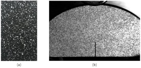
Figure 7.
Preparation of artificial speckles by spray painting the surface of the specimen: (a) speckle of non-cracked specimen; (b) speckle of NSCB specimen.
3.2. Test Equipment
As shown in Figure 8, this paper used the electronic universal testing machine (MTS-SANS CMT5504/5105, made in Shanghai, China, by MTS) to carry out the non-cracked cuboid thin plate test and the NSCB test. The equipment can apply a maximum load of 100 kN and set the loading speed to 0.06 mm/min. In the experiment, a digital camera (MV-VD500SM/SC, made in Xi’an, China, by Microvision) was used to record the development of the process zone near the crack and the crack expansion. For the non-cracked cuboid compression test and the NSCB test, the cameras were set to shoot the frequency of 10 and 2 per second, respectively. A roller-type loading fixture was used to carry out three-point bending loading to avoid side load on the specimen, and the loading form is shown in Figure 9.
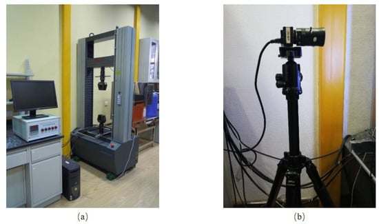
Figure 8.
Test equipment: (a) MTS electronic universal testing machine; (b) MV-VD500SM/SC digital camera.
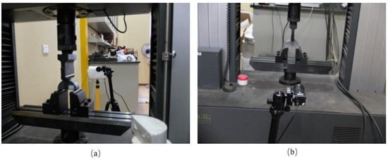
Figure 9.
Test loading diagram: (a) NSCB test with roller type three-point bending jig; (b) NSCB speckle side photographed with digital camera.
4. Test Results
4.1. Non-Cracked Compression Failure Test
The typical load-displacement curves of the three kinds of non-cracked shale specimens in the compression failure test are shown in Figure 10, and the peak load, maximum displacement, compressive strength, and elastic modulus of the test are summarized in Table 2.
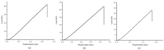
Figure 10.
Load-displacement diagram of the failure test that corresponds to three kinds of shale fracture modes: (a) splitter fracture corresponding to the failure test (S0); (b) arrester fracture corresponding to the failure test load-displacement diagram (A0); (c) divider fracture corresponding to the failure test (D0).
Table 2.
Compression test results of three modes of non-cracked shale specimens.
It can be seen from Table 2 that the compressive strength of the specimen S0 and the loading direction of D0 are parallel to the bedding, but both the compressive strength and elastic modulus of S0 are greater than that of D0; the elastic modulus of the specimen A0 is the smallest, but the compressive strength is the highest. In the test, DIC technology was used to observe the change characteristics of the speckle position on the surface of the test piece, and the NCORR software was used to analyze the distribution cloud map of horizontal and vertical displacement U, V, horizontal strain εx, and the vertical strain of each test piece before failure. The distribution cloud map of εy and shear strain εxy, i.e., the displacement field and strain field before shale failure under the three loading methods, are shown in Figure 11.
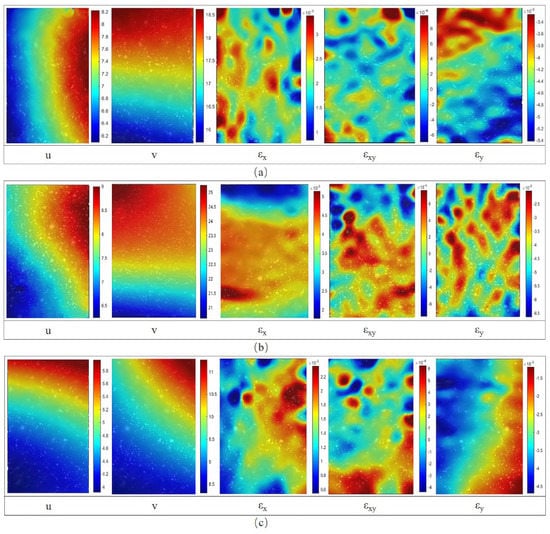
Figure 11.
Displacement field and strain field of each specimen before failure in the compression failure test without cracks: (a) specimen S0, (b) specimen A0, (c) specimen D0.
The corresponding unit of the displacement field is pixels, and each pixel of the test photo is about 0.02675 mm long. It can be seen from the observation that the specimen S0 was deformed by 8.2 pixels in the horizontal direction before the failure, i.e., 0.219 mm, and the vertical deformation was 18.7 pixels, i.e., 0.501 mm. The deformation was 25.5 pixels, i.e., 0.682 mm; before the specimen D0 was destroyed, the horizontal deformation was 5.9 pixels, or 0.158 mm, and 10.8 pixels in the vertical direction, or 0.289 mm. In terms of deformation amplitude, A0 was the highest, S0 was in the middle, and D0 was the lowest, which is related to the load level and the respective elastic modulus of the three before failure. The maximum horizontal-to-maximum vertical deformation ratios of S0, A0, and D0 before failure were 0.44, 0.35, and 0.52, respectively. Compared with shale, the Poisson’s ratio is generally higher than 0.33, particularly for specimens S0 and D0 with the loading direction parallel to the bedding direction. This indicates that shale is more prone to lateral deformation when subjected to loads parallel to the bedding direction before failure. The specimens are compressively deformed in the vertical direction, and the horizontal direction is tensile deformation due to the generalized Hooke’s law. The horizontal and vertical strains are of the same order of magnitude, and both of them are higher than the shear strain. The definition of the process zone implies that the deformation or stress conditions in the inner area of the process zone have reached or exceeded the strength limit of the material.
According to the second strength theory, starting from the strain, the maximum tensile strain that the non-fractured specimen can reach before failure is taken as the critical strain value of failure; thus, the process zone criterion is obtained. The region near the crack tip where the maximum principal strain value ε1 reaches or exceeds the material failure critical strain value εtc can be considered to be on the verge of failure or to have entered the nonlinear stage, i.e., it is within the fracture process region. According to the known εx, εy, and εxy, the maximum principal strain ε1 can be obtained by the following formula:
MATLAB was used to compile simple data processing commands, and the distribution data of εx, εy, and εxy obtained by the NCORR software were used to calculate the distribution data of the maximum principal strain ε1 of the specimen before failure and to visualize the calculation result as the maximum principal strain and distribute it in the cloud map, as shown in Figure 12.
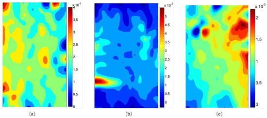
Figure 12.
Cloud map of the maximum principal strain distribution before the failure of the shale specimen without cracks: (a) ε1 distribution before splitter destruction (S0), (b) ε1 distribution before arrester destruction (A0), and (c) ε1 distribution before divider destruction (D0).
By observing Figure 12, it can be seen that the distribution cloud diagram of the maximum tensile strain ε1 has a large similarity with the horizontal strain εx of the specimen. Both values are positive, indicating that the tensile failure of the non-cracked specimen has occurred. These values have a high correlation with its horizontal strain. The maximum value of ε1 is the maximum principal strain that the non-cracked specimen can reach before failure at the corresponding temperature. According to the maximum tensile strain strength theory, these can be used as the failure critical strain value εtc of shale under different loading methods (as seen in Table 3).
Table 3.
The critical strain value of shale failure measured by the non-cracked compression test.
It can be seen from Table 3 that the critical strain value εtc of each specimen is of the same order of magnitude. The critical strain value of specimen A0 is relatively large, that of specimen D0 is relatively small, and that of specimen S0 is located between D0 and A0. Among the three loading conditions, when the shale is loaded by the arrester type, the local deformation that can be endured before failure is the largest, followed by the splitter type, and the divider type can bear the smallest deformation. According to the maximum tensile strain strength theory, when the rock strain reaches or exceeds the critical value εtc, it can be determined that the rock is on the verge of failure or has entered a nonlinear stage. So the critical strain value obtained in the compression failure tests can be used to delimit the fracture process zone from the principal strain distribution diagram obtained in the NSCB tests.
4.2. Fracture Toughness Test Results
After the fracture test, three kinds of classical NSCB test load-displacement diagrams for type-I fracture were obtained (Figure 13). It can be seen from the figure that the peak load of the divider type specimen was the highest, followed by the arrester type specimen, and the splitter type specimen was the smallest. The level of peak load indicates how easy it is for the specimen to break; thus, it is relatively more difficult for a divider to break.
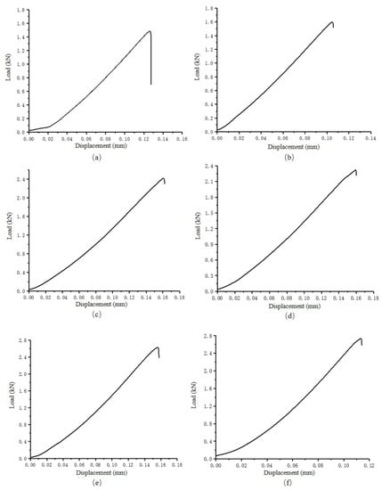
Figure 13.
NSCB test load-displacement diagram of three modes of type-I fractures in shale: (a) for the splitter fracture of specimen S1, (b) for the splitter fracture of specimen S2, (c) for the arrester fracture of specimen A1, (d) for the arrester fracture of specimen A2, (e) for the divider fracture of specimen D1, (f) for the divider fracture of specimen D2.
The type-I fracture toughness of NSCB specimens can be calculated by the standard Formula (7) recommended by ISRM:
where KIC is the type-I fracture toughness, Pmax is the peak load, a is the length of artificial prefabricated cracks, B is the thickness of the specimen, R is the radius of the semi-disk NSCB specimen, and Y′ is the infinite amount determined by the shape of the specimen and the loading conditions. In the recommended standard of ISRM, the calculation formula of Y′ under the condition of plane stress is given as follows:
where s is the span between the lower two pivot points in the three-point bending test, and β is the ratio of the thickness B to the radius R. In this test, s was set to 60 mm. After calculating Y’, the type-I fracture toughness of three different mode specimens was obtained (as in Table 4), and the average value of the results and related analysis data are listed in Table 5.
Table 4.
Type-I fracture toughness determined by the NSCB test for three kinds of shale specimen.
Table 5.
Statistics of NSCB test results for three kinds of shale specimen.
It can be seen that the fracture toughness of the divider specimens is the highest, the value of the splitter specimens is the lowest, and the fracture toughness of the arrester specimens is in the middle. This shows that, among the three typical modes of shale type-I fractures, divider fractures are the most difficult to expand, arrester fractures are the next most difficult, and splitter fractures are the easiest to expand.
The coefficient of variation of the type-I fracture toughness for the S-type specimens is significantly higher, and that of the A-type and D-type specimens is relatively low. This shows that, among the three typical types of shale type-I fracture specimens, the expansion degree of splitter fractures is quite different. This is probably due to the fact that the propagation direction of splitter fractures is parallel to the bedding plane of shale; thus, the fractures are often uniformly located in a specific bedding plane. The mechanical and fracture properties of the bedding plane have a great influence on the KIC of the splitter fracture. The fracture characteristics of the bedding planes near the fractures reflected by the KIC of the splitter fracture, even for the same batch of shale specimens, are quite different from each other due to the different bedding planes where the prefabricated fractures of specimens are located.
However, the expansion directions of the arrester and divider fractures are both perpendicular to the bedding plane, and their KIC is jointly affected by the many layers of shale. Therefore, the KIC of the same batch of shale arrester fractures and divider fractures will tend to reflect the overall fracture characteristics common to all bedding planes in this direction; thus, little difference exists in the test results of different shale specimens of the same fracture mode. It can be seen from Table 3 that the critical strain value εtc of each specimen is of the same order of magnitude. The critical strain value of specimen A0 is relatively large, that of specimen D0 is relatively small, and that of specimen S0 is located between D0 and A0. Among the three loading conditions, when the shale is loaded by the arrester type, the local deformation that can be endured before failure is the largest, followed by the splitter type, and the divider type can bear the smallest deformation. According to the maximum tensile strain strength theory, when the rock strain reaches or exceeds the critical value εtc, it can be determined that the rock is on the verge of failure or has entered a nonlinear stage.
4.3. Fracture Mechanism
According to the order in which the speckle photos were collected and compared with the fracture time of the sample observed in the experiment, three photos corresponding to the fracture time were chosen from many photos, which were defined as before the fracture, during the fracture, and after the fracture. By inputting the speckle photos at various stages in the test process, the latter photo was only slightly deformed compared to the previous photo, so that the NCORR software could accurately match according to its internal algorithm and then compare the speckle before the fracture. The differences between the photo and the no-load reference speckle photo, the distribution cloud map of the horizontal displacement V, vertical displacement U, horizontal strain εy, vertical strain εx, and shear strain εxy of each specimen before the fracture occurred are shown in Figure 14, Figure 15 and Figure 16; the displacement field and strain field of a typical specimen before failure and the speckle photos taken before and after failure are shown under the three loading methods.
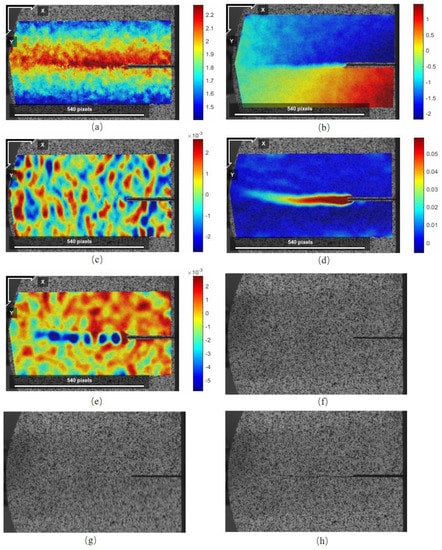
Figure 14.
Displacement field, strain field, and photos of specimen S2 before and after fracture: (a) distribution field of vertical displacement U before the occurrence of the S2 fracture; (b) distribution field of horizontal displacement V before the occurrence of the S2 fracture; (c) distribution field of strain εx before the occurrence of the S2 fracture; (d) distribution field of strain εy before the occurrence of the S2 fracture; (e) distribution field of strain εxy before the occurrence of the S2 fracture; (f) photo before the occurrence of the S2 fracture (the original 2932th photo); (g) photo during the occurrence of the S2 fracture (the original 2933th photo); (h) photo after the S2 fracture (the original 2934th photo).
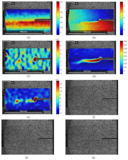
Figure 15.
Displacement field, strain field, and photos of specimen A2 before and after the fracture: (a) distribution field of vertical displacement U before the occurrence of the A2 fracture; (b) distribution field of horizontal displacement V before the occurrence of the D2 fracture; (c) distribution field of strain εx before the occurrence of the A2 fracture; (d) distribution field of strain εy before the occurrence of the A2 fracture; (e) distribution field of strain εxy before the occurrence of the A2 fracture; (f) photo before the occurrence of the A2 fracture (the original 4401th photo); (g) photo during the occurrence of the A2 fracture (the original 4402th photo); (h) photo after the A2 fracture (the original 4403th photo).
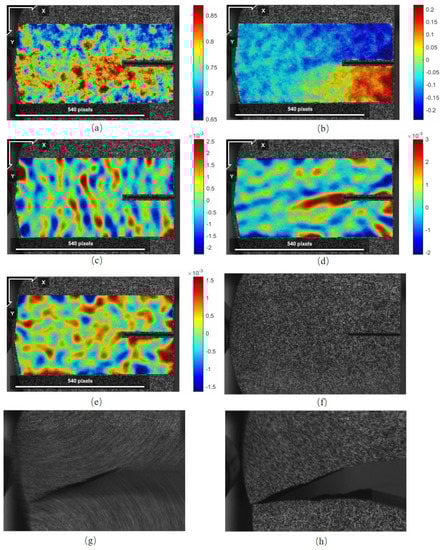
Figure 16.
Displacement field, strain field, and photos of specimen D2 before and after the fracture: (a) distribution field of vertical displacement U before the occurrence of the D2 fracture; (b) distribution field of horizontal displacement V before the occurrence of the D2 fracture; (c) distribution field of strain εx before the occurrence of the D2 fracture; (d) distribution field of strain εy before the occurrence of the D2 fracture; (e) distribution field of strain εxy before the occurrence of the D2 fracture; (f) photo before the occurrence of the D2 fracture (the original 3057th photo); (g) photo during the occurrence of the D2 fracture (the original 3058th photo); (h) photo after the D2 fracture (the original 3059th photo).
When the NCORR software processes the speckle image, the unit of the output displacement field is pixel. Taking the line segment with a length of 540 pixels in Figure 16 as the reference, the length of each pixel of the NSCB test photo was calculated to be about 0.055 mm. Based on this, the strain field at the crack tip of the specimen was analyzed, and it was found that the horizontal strain εy near the prefabricated crack tip before the fracture was significantly larger than the vertical strain εx and shear strain εxy, indicating that the region near the tip was mainly deformed in the horizontal direction (perpendicular to the crack direction). The shape of the high-strain region on the horizontal strain εy distribution map had a certain similarity with the shape of the new macroscopic crack after the fracture occurred.
By observing the shear strain cloud map of each specimen, it was found that the high shear strain zone of almost all specimens was located in the process zone, the shear strain amplitude was significantly different from the surrounding area, and there were also many adjacent high shear strain zones. Regarding the obvious spacing, its overall distribution shape resembles a string of beads connected in a line; thus, it may be called a beaded high shear strain area. Comparing the crack morphology of the specimen after the fracture occurred, it could be seen that the beaded high shear strain area was especially obvious in the area where the macroscopic crack was bent and deflected. The positive and negative of the beaded high-shear strain region εxy was highly correlated with the spatial variation of the shape of the high-strain region on the horizontal strain εy distribution map.
Some of the beaded high shear strain zones εxy of the S-type specimens had positive values, and the shape of the high strain regions on the horizontal strain εy distribution map was downwardly inclined, with some having negative values. The shape of the high strain area was upwardly biased. However, the beaded high shear strain zone εxy of the A-type specimen was generally positive, and the shape of the high-strain region on the horizontal strain εy distribution map was downwardly inclined; the “bead- shaped” high shear strain zone of the D-type specimen was along the crack. In the expansion direction, the first shear strain was negative (negative bead), and the shear strain εxy was positive, indicating that the specimen had both clockwise and counter-clockwise shear deformations before the fracture. Correspondingly, the shape of the high-strain region in the horizontal strain εy distribution graph was first upward and then downward.
It was concluded that the crack propagation distance of different specimens was different a short time after the fracture occurred, the S-type specimen had the shortest crack propagation distance, the A-type specimen had the second longest, the D-type specimen had the longest, and most specimens had cracks. The extension distance was similar to the length of its process zone. The crack propagation distance of individual D-type specimens (such as specimen D2) far exceeded the length of its process zone, and even reached the specimen boundary. It can be inferred from the speed at which the specimen broke that if the size of the specimen can be increased, the potential crack propagation distance can be beyond the boundary of the original specimen.
5. Discussion
5.1. FPZ Features
The data of the distribution cloud map of the horizontal displacement V, vertical displacement U, horizontal strain εy, vertical strain εx, and shear strain εxy before the expansion of prefabricated cracks in each specimen were stored in NCORR in the form of a data matrix. In the output m file, the maximum principal strain ε1 of each NSCB specimen was calculated with the help of MATLAB software, and the maximum principal strain distribution map before fracture of each specimen was also obtained (Figure 17).
For the maximum principal strain distribution map of each group of specimens, the maximum value of the color bar was set to the corresponding failure critical strain value in Table 3. In the new distribution map, the areas where the maximum principal strain exceeded the critical value were marked as the same color, reddish brown. According to the second strength theory, the area where the maximum principal strain exceeded the critical strain value was already in the damaged state (or yield state, plastic stage); thus, these reddish-brown areas can be considered the FPZ at the crack tip. The FPZ at the crack tip of each specimen is visually displayed in Figure 17.

Figure 17.
Maximum principal strain distribution and FPZ of the NSCB specimen before the fracture: (a) distribution diagram for the splitter fracture (specimen S1); (b) splitter FPZ (specimen S1); (c) distribution diagram for the shale splitter fracture (specimen S2); (d) splitter FPZ (specimen S2); (e) distribution map for the shale arrester fracture (specimen A1); (f) arrester FPZ (specimen A1); (g) distribution map for the shale arrester fracture (specimen A2); (h) arrester FPZ (specimen A2); (i) distribution map for the shale divider fracture (specimen D1); (j) divider FPZ (specimen D1); (k) distribution map for the shale divider fracture (specimen D2); (l) divider FPZ (specimen D2).
By comparing the maximum principal strain distribution and FPZ of different types of specimens, it can be seen that, before the fracture of all specimens, the FPZ was generally narrow and long, and the shape was similar to a flame. There is a big difference between the “fire-shaped” process zone in the real situation, the “apple-shaped” process zone calculated under ideal conditions in Figure 2, and the “peach-shaped” process zone in Figure 3 considering stress relaxation. This paper believes that the reason for the difference is that the rock-like materials have obvious directionality due to the stress relaxation in the process zone. The shape of the process zone of each specimen was highly similar to the high-level directional strain area in Figure 14, Figure 15 and Figure 16, and it was also very close to the macroscopic new crack shape after the fracture occurred, indicating that the occurrence of the fracture was highly related to the horizontal direction strain. Except for individual D-type specimens (D2), the length of the process zone for other specimens differed little. The process zone of these specimens was small, the crack propagation distance was long, and the crack extended beyond the process zone or even beyond the boundary of the specimen, which is inconsistent with the description of the fracture process stage E in the traditional fracture process theory. In the process zone, the closer the vertical direction is to the crack tip and the closer the horizontal direction is to the area of the new crack after the fracture occurs, the greater the maximum principal strain, i.e., the greater the tensile deformation strength. The image of the FPZ at the crack tip of each specimen in Figure 17 was measured, and the relevant geometric dimension indicators of the process zone of different specimens are shown in Table 6:
Table 6.
The geometric size index of the process zone for three modes of specimens.
From Table 6 and Figure 17, it can be seen that the maximum height, range height, and range length of the FPZ at the crack tip before the fracture of different specimens were quite different, and whether there was obvious bending deflection between the new crack and the prefabricated crack after the fracture was also different. Among them, the maximum height and range height of the FPZ of the crack tip of the S-type specimen before the fracture occurred were small, but the length of the process zone was not much different from the other types of specimens. Therefore, the height-to-length ratio of the process zone of the S-type specimen was relatively low (about 0.17), and there was no obvious bending deflection between the new crack and the prefabricated crack after the fracture occurred.
The maximum height and range height of the FPZ at the crack tip of the A-type specimen were relatively large before the fracture occurred. Therefore, the height-to-length ratio of the process zone of the A-type specimen was generally high (about 0.25), and there was obvious bending deflection between the new crack and the prefabricated crack after the fracture occurred. The height-to-length ratio of the process zone of the D-type specimen was obviously larger than that of other types of specimens, while the specimen D1 was not much different from the S-type specimen. Therefore, the height-to-length ratio of the process zone of the D-type specimen also varied within a large range (0.17~0.38).
The specimen D1 with a low height-to-length ratio in the process zone had no obvious bending deflection between the new crack and the prefabricated crack after the fracture. However, the specimen D2 with a high height-to-length ratio in the process zone had obvious bending between the new crack and the prefabricated crack after the fracture occurred.
By comparing the fracture characteristics of S-type, A-type, and D-type shale specimens, it was found that there was no significant difference in the extent length of the extended process zone of the splitter fracture, but the maximum height, the extent height, and the extent height-to-length ratio were smaller, and the probability of bending deflection between new cracks and prefabricated cracks after the fracture was smaller. No significant difference existed in the extent length of the expansion process zone of the arrester fracture, but it had a larger maximum height of the process zone, the extent height, and the range height-to-length ratio. The probability of bending deflection between the new crack and the prefabricated crack after the fracture was the highest among the three expansion modes. There was no significant difference in the extent length of the extended process zone of the divider fracture, and it had a relatively large maximum height of the process zone, area height, and range height-to-length ratio. The probability of bending deflection between the new crack and the prefabricated crack after the divider fracture was between the splitter fracture and the arrester fracture. Generally speaking, whether the bending deflection occurs between the new crack and the prefabricated crack after the fracture occurs mainly depends on the height-to-length ratio of the FPZ at the crack tip, which is not highly correlated with the maximum height and range length of the process zone, but it has a certain correlation with the range height.
5.2. Analysis of Crack Propagation Mechanism
In order to compare the shear strain distribution fields of different types of specimens more conveniently, the shear strain cloud diagrams of typical specimens are drawn in Figure 18.
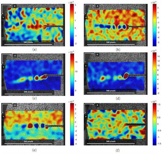
Figure 18.
The distribution field of shear strain εxy before the fracture of different NSCB specimens: (a) εxy for S1; (b) εxy for S2; (c) εxy for A1; (d) εxy for A2; (e) εxy for D1; (f) εxy for D2.
For individual D-type specimens, the range of high strain in the horizontal direction εy was obviously small, and the shear strain εxy did not have a beaded distribution, indicating that the size of the FPZ was small. It was found that, in the photos taken by the high-speed camera, there was a certain blurred area along the direction of the crack extension, indicating that the two sides of the crack deviated from each other at a relatively high speed at this time (Figure 16). At the same time, it was observed that the deviation of both sides of the fracture was large and the speed was fast; the newly formed fracture was straight, but there was a bending phenomenon between the fracture and the prefabricated fracture. It can be explained that the direction re-selection of fractures may occur in the development stage of the process zone, but it is not easy to change direction in the stage of rapid intrusion and expansion of fractures. In addition, according to the statistics of the shooting time, the specimen completed crack initiation and penetration within 0.1 s and was completely destroyed. Combined with the load-displacement curve, it can be inferred that the specimen with a small size in the fracture process zone or no obvious beaded high shear strain zone has high brittleness or strong bursting liability. The brittleness of shale is one of the three key parameters used to evaluate the fracability of shale gas reservoirs [26,27], and strong bursting liability is an important parameter used to evaluate the possibility of rock burst in underground engineering, especially in coal mines [28,29]. The observation results suggest that the size of the fracture process zone before fracture propagation is very likely to be negatively correlated with the strength of the fracture impact, and there may be a new method to measure brittleness or impact propensity by observing the pre-crack strain field and fracture process zone around the crack tip.
Combined with the distribution characteristics of fracture toughness of different types of specimens in Table 4 and the cloud diagram of continuous bead shear strain, it can be seen that the peak load and the type-I fracture toughness of the S-type specimens were low, the “bead” formed before the fracture was smaller and denser, and the amplitude of the shear strain in this region was also relatively low. The peak load and the type-I fracture toughness of the A-type and D-type specimens were relatively high, the “connected bead type” before the fracture was larger and sparser, and the amplitude of the shear strain in the “connected beaded type” region was higher. It can be seen that the size and density of the “bead “ area were greatly affected by the relationship between the direction of the fracture propagation and shale bedding. However, there was a high correlation between the amplitude of shear strain in the “bead” region and the height-to-length ratio of the process region. Whether the bending deflection occurs between the new crack and the original prefabricated crack after the fracture mainly depends on the height-to-length ratio of the FPZ at the crack tip. Therefore, it can be considered that the magnitude of the shear strain in the “bead” region determines whether the new crack will bend or deflect relative to the original crack.
Combined with the fracture morphology of each specimen (Figure 14, Figure 15 and Figure 16), it was found that the new cracks generated after the fracture can well connect the beaded high shear strain zones before the fracture, and these beaded distributions of high shear strain areas mostly occur in the bending and deflection of new cracks. It can be concluded that there is a very close relationship between the new fractures and the beaded distribution of high shear strain zones. The author believes that the reason for the appearance of the high shear strain zone of the beaded distribution is that micro-fractures exist in the process zone of the fracture tip, and the micro-fractures are connected with each other before the fracture, forming a connected area and small shear deformation. The mutually overlapping regions are deflected towards each other, resulting in the formation of high shear strain zones in the interconnected regions.
The FPZ at the fracture tip of the fractured rock structure subjected to type-I static loading can be divided into three stages from development to fracture propagation (Figure 19). When the cracked rock is subjected to type-I static loading, the stress concentration at the crack tip is much larger than that in the surrounding area. Due to the uneven distribution of tensile strength everywhere, as the load increases, the weak areas near the crack tip begin to fracture one after another and create micro-cracks. Since the positions of these weak areas are randomly distributed, the newly generated micro-cracks in the process zone are also randomly distributed. The tensile stress is dominant in the whole process zone, and the main direction of the random microcracks is perpendicular to the loading direction.
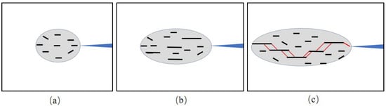
Figure 19.
The three stages of the type-I crack structure from static loading to crack propagation: (a) there is stress concentration at the crack tip, and micro-cracks and the process zone appear; (b) the load continues to increase, the number of micro-cracks increases, and the process zone becomes larger; (c) when the load reaches the peak value, the micro-cracks penetrate each other, new macroscopic cracks appear, and the cracks expand.
In the early stages of the development of the process zone, the micro-fractures that are parallel to each other and are located in different positions have a low degree of development, their expansion is subcritical, and the influence on each other can be ignored. Fractures with vertical directions are more likely to develop and expand. As the load increases, the process zone gradually increases, and the fractures that are parallel to each other but randomly located gradually develop and grow. The expansion of micro-cracks at this stage belongs to subcritical expansion, and the structural stiffness will decrease to a certain extent due to the increase of cracks, but the overall bearing capacity will not greatly decrease with the expansion of cracks.
There will be interactions between adjacent cracks, but the propagation direction of micro-cracks is still mainly determined by the direction of the external load. At this stage, it can be seen that the micro-fractures show an “echelon” distribution. Subsequently, when the parallel but non-collinear geese micro-fractures in the process zone continue to grow and overlap each other, the interaction between adjacent micro-fractures will affect the direction of fracture propagation. The micro-fractures change from pure type-I expansion to I-II compound-type expansion. In the overlapping area, the two adjacent echelon-type cracks no longer continue to expand perpendicular to the loading direction, but are centro-symmetrically deflected and expanded toward the adjacent cracks.
This leads to the interpenetration of the originally parallel but non-collinear microcracks. With the deflection of the propagation direction of microfractures, the rocks in the overlapping area of adjacent microfractures also undergo shear deformation, resulting in the appearance of high shear strain zones. As shown in Figure 19, when the high shear strain zone is distributed in a bead shape, it means that multiple micro-cracks in the process region are connected to each other to form new macro-cracks. The size of the crack will be equivalent to the total length of the beaded high shear strain zone, which will have a non-negligible effect on the crack-containing structure.
It was found that there were both positive shear strain beads and negative shear strain beads in the shear strain distribution diagram of some specimens. The positive and negative shear strains were very close in absolute value, indicating that both clockwise and counterclockwise shear deformations existed before the fracture. The positive or negative of the strain amplitude in the high shear strain zone is determined by the positional relationship between the adjacent micro-cracks that are about to penetrate. The distribution of echelon-shaped micro-cracks is random, and the shear deformation before interconnection is clockwise or counter-clockwise, which is also random. The positive and negative arrangement of beaded high shear strain areas in the FPZ at the crack tip is the “mutual cancellation” of shear deformation in this area. Therefore, there is no obvious bending direction between the new macro-cracks formed by the mutual penetration of the micro-cracks in this area and the prefabricated cracks.
Since the interconnection between adjacent micro-fractures is centrosymmetric, clockwise or counter-clockwise can be used to distinguish their interrelationships. As shown in Figure 20, if the crack on the right is under the adjacent crack on the left, then the deflection of the crack is clockwise when they are connected to each other, and the shear strain in the diamond-shaped area surrounded by the cracks is positive (marked in red in the Figure 20). If the fracture on the right is above the adjacent fracture on the left, then the deflection of the fracture is counterclockwise when they are interconnected, and the shear strain in the diamond-shaped region is negative (marked in blue).
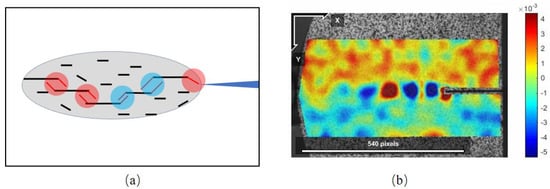
Figure 20.
The schematic diagram of the origin of the high shear strain with beaded distribution: (a) the micro−cracks in the process zone are connected to each other to form a high shear strain area; (b) the high shear strain area with a beaded distribution.
The micro-fractures that develop separately in the process zone lead to shear deformation in the area between the fractures (the diamond-shaped area in Figure 20a) when they are interconnected. When a high shear strain zone with a beaded distribution appears in the process zone at the tip of the type−I crack, it means that the micro-cracks are connected to each other at multiple places that can be connected in a line in the process zone at the same time. Multiple high shear strain zones are connected in a series to form a “connection line”, which can basically be regarded as a new crack after the fracture occurs. This is a through-type macroscopic crack, which will greatly change the structural stiffness.
5.3. Engineering Significance of Beaded High Shear Strain Zone
The tensile strength of the rock is low, and the main direction of the micro-cracks generated in the process zone is mostly parallel to the direction of crack propagation, resulting in the stress relaxation in the process zone also having obvious directionality. This makes the process zone extend longer in the direction parallel to the crack propagation direction and inconspicuous in the direction perpendicular to the crack propagation direction, forming a flame-shaped process zone. The appearance of the beaded high shear strain zone indicates that the interaction between multiple micro-cracks in the region accelerates the penetration of micro-cracks, resulting in the appearance of macro-cracks. Therefore, the appearance of the beaded high shear strain zone indicates that the type I fracture is about to expand.
When carrying out some displacement monitoring or strain monitoring in engineering, special attention should be paid to the phenomenon of high shear strain area with continuous beaded distribution. The engineering rock mass itself is a body with cracks. The appearance of finite cracks often has a limited impact on the bearing capacity of the rock mass. However, the appearance of a beaded high shear strain area means that multiple cracks are connected to each other at the same time. The simultaneous interconnection of such multiple cracks will greatly change the overall stiffness of the structure in a very short period of time, which may easily lead to disaster. Therefore, by monitoring the strain field of the key parts of the engineering rock mass and analyzing the specific location of the beaded high shear strain area, the location and timing of dynamic instability can be predicted to play a preventive or early warning role.
6. Conclusions
In this paper, shale compression failure tests and NSCB tests were carried out, and, with the help of DIC technology, the critical strain values of different failure modes of shale were obtained. Then, intuitive distribution maps of strain and fracture process zones around the prefabricated fracture tip before the fracture propagation were created. By comparing the fracture process zone distribution maps and test results of different types of shale specimens, it was found that different types of shale specimens have different crack deflection probabilities. The deflection probability of A-type specimens is the largest, followed by D-type specimens, and the deflection probability of S-type specimens is the lowest.
The fracture process zone of shale observed in the tests was narrow and long with a shape similar to a flame. It was quite different from the short and round fracture process zone obtained by theoretical calculation, which may have been induced by the microcracks whose directions were close to those of prefabricated cracks and inhomogeneous stress relaxation in the fracture process zone. Whether the bending deflection occurs between the new crack and the prefabricated crack after the fracture occurs has a high correlation with the height-to-length ratio of the fracture process area around the crack tip.
The crack propagation of most specimens after the fracture is confined to the range of the fracture process zone, but the fracture process zone size of a few samples was significantly smaller than that of the others. The failure impact of these samples was significantly stronger, so that the crack propagation exceeded the range of the fracture process zone. The observation results suggest that the size of the fracture process zone before fracture propagation is very likely to be negatively correlated with the strength of the failure impact.
In most of the specimens, a beaded high shear strain zone appeared in the distribution map of shear strain fracture before the fracture propagation. The beaded high shear strain zone is caused by the oblique communication of micro-fractures distributed in a “geese-pattern” in the fracture process zone before the fracture. The appearance of a beaded high shear strain zone indicates that the interconnection between different microcracks is intensified and that macrocracks are about to occur.
The research conclusions can be used for predicting the direction and shape of crack propagation, estimating the brittleness or bursting liability of rock, and disaster early warning and prevention.
Author Contributions
Conceptualization, T.T.; methodology, T.T. and X.S.; formal analysis, T.T. and X.S.; investigation, T.T., X.S. and X.Z.; writing-original draft preparation, T.T. and L.L.; writing-review and editing, X.S. and X.Z.; visualization, T.T. and X.S.; supervision, L.L.; funding acquisition, T.T., X.S. and X.Z. All authors have read and agreed to the published version of the manuscript.
Funding
This research was supported by the Innovation and Entrepreneurship Science and Technology Special Project of Coal Research Institute [grant No. 2021-KXYJ-002], China Coal Science and Industry Group Co., Ltd. Technology Innovation and Entrepreneurship Fund Special Project [grant No. 2022-2-QN002], Science and Technology Development Fund Project of China Coal Research Institute [grant No. 2021CX-II-11].
Acknowledgments
The authors gratefully acknowledge test equipment and technical support provided by Da’an Liu, Rock Fracture Mechanics Specialist, Institute of Geology and Geophysics, Chinese Academy of Sciences, Beijing.
Conflicts of Interest
The authors declare no conflict of interest.
References
- Bai, B.; Elgmati, M.; Hao, Z.; Wei, M. Rock characterization of Fayetteville shale gas plays. Fuel 2013, 105, 645–652. [Google Scholar] [CrossRef]
- Guo, Z.; Li, X.; Liu, C. Anisotropy parameters estimate and rock physics analysis for the Barnett Shale. J. Geophys. Eng. 2014, 11, 065006. [Google Scholar] [CrossRef]
- Josh, M.; Esteban, L.; Piane, C.D.; Sarout, J.; Dewhurst, D.N.; Clennell, M.B. Laboratory characterisation of shale properties. J. Pet. Sci. Eng. 2012, 88–89, 107–124. [Google Scholar] [CrossRef]
- Bayuk, I.O.; Ammerman, M.; Chesnokov, E.M. Upscaling of elastic properties of anisotropic sedimentary rocks. Geophys. J. R. Astron. Soc. 2010, 172, 842–860. [Google Scholar] [CrossRef]
- Banik, N.C. Velocity anisotropy in shales and depth estimation in the North Sea Basin. Geophysics 1984, 49, 15. [Google Scholar] [CrossRef]
- Lekhnitskii, S.G. Radial distribution of stresses in a wedge and in a half-plane with variable modulus of elasticity. J. Appl. Math. Mech. 1962, 26, 199–206. [Google Scholar] [CrossRef]
- Wardle, L.J.; Gerrard, C.M. The “equivalent” anisotropic properties of layered rock and soil masses. Rock Mech. 1972, 4, 155–175. [Google Scholar] [CrossRef]
- Salamon, M. Elastic moduli of a stratified rock mass. Int. J. Rock Mech. Min. Sci. Geomech. Abstr. 1968, 5, 519–527. [Google Scholar] [CrossRef]
- Amadei, B. Importance of anisotropy when estimating and measuring in situ stresses in rock. Int. J. Rock Mech. Min. Sci. Geomech. Abstr. 1996, 33, 293–325. [Google Scholar] [CrossRef]
- Kwasniewski, M.; Neuyen, H.V. Experimental studies on anisotropy of time-dependent behaviour of bedded rocks. In Proceedings of the International Symposium on Engineering in Complex Rock Formations, Beijing, China, 1 January 1988; pp. 325–337. [Google Scholar]
- Pinto, J.L. Deformability of schistous rocks. In Proceedings of the International Society of Rock Mechanics, Bergama, Turkey, 21 September 1970. [Google Scholar]
- Read, S.; Perrin, N.D.; Brown, I.R. Measurement and Analysis of Laboratory Strength and Deformability Characteristics of Schistose Rock. In Proceedings of the ISRM Congress, Montreal, QC, Canada, 3 September 1987. [Google Scholar]
- Pomeroy, C.D.; Hobbs, D.W.; Mahmoud, A. The effect of weakness-plane orientation on the fracture of Barnsley Hards by triaxial compression. Int. J. Rock Mech. Min. Sci. Geomech. Abstr. 1971, 8, 227–238. [Google Scholar] [CrossRef]
- Wang, H.; Wang, Z.; Wang, J.; Wang, S.; Wang, H.; Yin, Y.; Li, F. Effect of confining pressure on damage accumulation of rock under repeated blast loading. Int. J. Impact Eng. 2021, 156, 103961. [Google Scholar] [CrossRef]
- Shi, X.; Zhao, Y.; Gong, S.; Wang, W.; Yao, W. Co-effects of bedding planes and loading condition on Mode-I fracture toughness of anisotropic rocks. Theor. Appl. Fract. Mech. 2022, 117, 103158. [Google Scholar] [CrossRef]
- Ke, C.C. Determination Fracture of Anisotropic Rocks Boundary Element Method. Rock Mech. Rock Eng. 2008, 41, 509–538. [Google Scholar] [CrossRef]
- Kenner, V.H.; Advani, S.H.; Richard, T.G. A Study of Fracture Toughness for an Anisotropic Shale. In Proceedings of the US Symposium on Rock Mechanics, Berkeley, CA, USA, 25–27 August 1982. [Google Scholar]
- Schmidt, R.A. Fracture Mechanics of Oil Shale-Unconfined Fracture Toughness, Stress Corrosion Cracking and Tension Test Results. In Proceedings of the 18th U.S. Symposium on Rock Mechanics, Keystone, CO, USA, 22–24 June 1977. [Google Scholar]
- Shi, X.S.; Yao, W.; Liu, D.; Xia, K.W.; Tang, T.W.; Shi, Y.R. Experimental study of the dynamic fracture toughness of anisotropic black shale using notched semi-circular bend specimens. Eng. Fract. Mech. 2019, 205, 136–151. [Google Scholar] [CrossRef]
- Timoshenko, S.P. Strength of Materials; D. Van Nostrand Company, Inc.: New York, NY, USA, 1940. [Google Scholar]
- Rickman, R.; Mullen, M.; Petre, E.; Grieser, B.; Kundert, D. A Practical Use of Shale Petrophysics for Stimulation Design Optimization: All Shale Plays Are Not Clones of the Barnett Shale. In Proceedings of the SPE Annual Technical Conference & Exhibition, Denver, CO, USA, 21–24 September 2008; Society of Petroleum Engineers: Richardson, TX, USA, 2008. [Google Scholar]
- Liu, D.A.; Shi, X.; Zhang, X.; Wang, B.; Tang, T.; Han, W. Hydraulic fracturing test with prefabricated crack on anisotropic shale: Laboratory testing and numerical simulation. J. Pet. Sci. Eng. 2018, 168, 409–418. [Google Scholar] [CrossRef]
- Nakano, M.; Kishida, K.; Yamauchi, Y.; Sogabe, Y. Dynamic fracture initiation in brittle materials under combined mode I/II loading. J. Phys. 1994, 4, 695–700. [Google Scholar] [CrossRef][Green Version]
- Atkinson, C.; Smelser, R.E.; Sanchez, J. Combined mode fracture via the cracked Brazilian disk test. Int. J. Fract. 1982, 18, 279–291. [Google Scholar] [CrossRef]
- Irwin, G.R. Analysis of Stresses and Strains Near End of a Crack Traversing a Plate. J. Appl. Mech. 1956, 24, 361–364. [Google Scholar] [CrossRef]
- Yuan, J.L.; Deng, J.G.; Zhang, D.Y.; Li, D.H.; Yan, W.; Chen, C.G.; Cheng, L.G.; Chen, Z.J. Fracability evaluation of shale-gas reservoirs. Acta Pet. Sin. 2013, 34, 523–527. [Google Scholar]
- Tang, Y.; Xing, Y.; Li, L.Z.; Zhang, B.H.; Jiang, S.X. Influence factors and evaluation methods of the gas shale fracability. Earth Sci. Front. 2013, 19, 356–363. [Google Scholar]
- Pan, Y.S.; Dai, L.P. Theoretical formula of rock burst in coal mines. J. China Coal Soc. 2021, 46, 789–799. [Google Scholar]
- Ju, W.J.; Lu, Z.G.; Gao, F.Q.; Zhao, Y.X.; Li, W.Z.; Sun, Z.Y.; Hao, X.J. Research progress and comprehensive quantitative evaluation index of coal rock bursting liability. Chin. J. Rock Mech. Eng. 2013, 40, 1839–1856. [Google Scholar]
Publisher’s Note: MDPI stays neutral with regard to jurisdictional claims in published maps and institutional affiliations. |
© 2022 by the authors. Licensee MDPI, Basel, Switzerland. This article is an open access article distributed under the terms and conditions of the Creative Commons Attribution (CC BY) license (https://creativecommons.org/licenses/by/4.0/).