Medium-Voltage Distribution Network Parameter Optimization Using a Thyristor Voltage Regulator

Abstract

The article is devoted to the study of steady-state conditions of a distribution network containing a thyristor voltage regulator. The thyristor voltage regulator (TVR) is a new controlled semiconductor device developed at Nizhny Novgorod State Technical University n.a. R.E. Alekseev (NNSTU). The TVR allows the optimization of the parameters of 6–20 kV distribution networks (currents and voltages) by voltage regulation. An analytical calculation of electromagnetic processes of a distribution network with the TVR has been carried out. The verification of the obtained results has been made using a computer simulation. The dependences of the current and power on additional voltage introduced by the TVR under different voltage regulation modes have been obtained. It has been shown that the use of the TVR enables optimal flow distribution to be ensured over the power transmission lines in proportion to their transfer capability when changing load power and its power factor.

1. Introduction

Modern medium-voltage distribution networks (DNs) are characterized by a number of problems [1,2,3]. As a rule, step-down substations (SSs) 35–220/6–20 kV are significantly far from transformer substations (TSs) 6–20/0.4 kV. This leads to a voltage level decrease at TS 6–20/0.4 kV and, as a consequence, to the quality loss of power supply to low-voltage consumers [4]. Medium-voltage transmission lines are often characterized by a nonoptimal power flow distribution along parallel lines, and, as a result, a limited transfer capability, increased power and electricity losses, and increased power transmission costs [5,6]. Weak medium-voltage DN interconnections limit the energy exchange between the energy market subjects. First, it leads to profit decreases for generating companies, and secondly, it reduces the electromagnetic compatibility of small-scale generation devices, and renewable and nontraditional energy sources with the network. In addition, such networks are characterized by low regime controllability [7].

Most of these problems can be solved by using flexible alternating current transmission system (FACTS) technologies [8,9]. At the same time, automated devices for voltage regulation have been introduced into the electrical network [10,11,12,13,14,15]. One of such devices is the thyristor voltage regulator (TVR), developed at NNSTU [16,17]. The TVR can operate in the voltage magnitude, phase angle, and combined control modes.

Figure 1 shows a single-line diagram of the DN with the TVR. The purpose of the TVR is to regulate the network parameters with different nominal voltages (110 and 10 kV). A connection between 110 and 10 kV networks is carried out using 16,000 kVA 110/10 kV ONAF transformers located at step-down substations SS1 and SS2. The 110 kV network and the 10 kV distribution network have different power-line lengths and impedances. They are not loaded in proportion to their transfer capability. Load node voltages may differ from the regulated values.

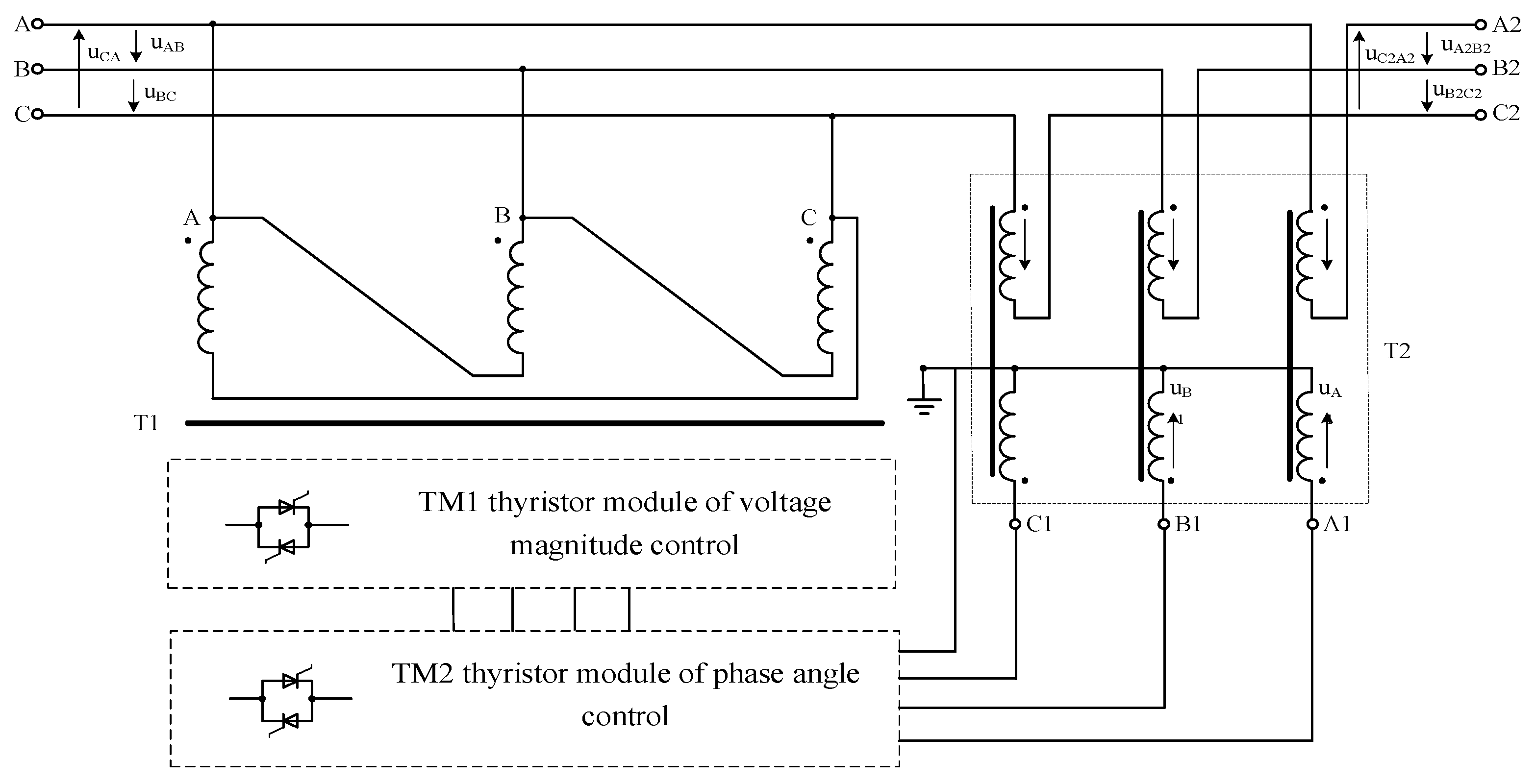
Figure 2 shows the TVR electrical circuit diagram.

The TVR includes thyristor modules of voltage magnitude (TM1) and phase angle (TM2) control, parallel T1 and series T2 transformers, and a control system. The TM1 and TM2 modules of each phase of the TVR contain regulation sections switched by thyristor switches. The output voltages of regulation modules feed the primary windings of transformer T2. Additional voltage is introduced into the line by the T2 secondary windings. The use of the pulse-phase control with the combined use of TM1 and TM2 modules allows one to change smoothly the output voltage magnitude and phase in the required range [18].

It is possible to load power lines with different parameters in proportion to their transfer capability by changing the magnitude and phase of the TVR additional voltage vector. It is also possible to control the directions of the real and reactive power flows of different parts of the network by voltage magnitude and phase angle control. It allows one to optimize the operation modes at the substations, reducing the losses of the DN parts by partial compensation of the current reactive component.

The article is devoted to the study of the TVR influence on the power and current values and directions in a medium-voltage distribution network under steady-state network conditions.

2. Methods

The research requires the development of adequate analytical models. There are different approaches to modeling steady-state network conditions. One way is to compile and calculate a single-line-equivalent circuit for a network. In this case, lines, transformers, and voltage regulators are represented by their equivalent circuits consisting of branches with conductivities and power sources.

A calculating technique for steady-state DN conditions using the graph and matrix theories has been developed. This approach allows one to write compactly and solve the equations of the circuit.

The calculation algorithm is as follows:

1. Determining assumptions.

2. Drawing up a DN-equivalent circuit.

3. Determining the parameters of the DN-equivalent circuit elements.

4. Referring the parameters of the transmission line to the base voltage.

5. Drawing up a directed graph that repeats the graphical representation of the circuit.

6. Drawing up an incidence matrix. The incidence matrix defines the connection between the nodes and branches. It consists of «0» and «1». The lines are assigned to the graph nodes. Each row of the linked graph has at least one «1». It indicates if there is a connection between the corresponding node and the branches of the graph. If there is a connection, then «1» is set. The «+» sign means that the direction is set from the node, and the «–» sign means the direction is set to the node.

7. Calculating the steady-state conditions by the node voltage method, taking nodal potentials as unknown:

$$\stackrel{•}{\mathsf{\phi }}=-{(A{\stackrel{•}{Y}}_d{A}^T)}^{-1}A{\stackrel{•}{Y}}_{d}E,$$

(1)

where A is the nodal matrix (incident matrix) of the circuit; ${\stackrel{•}{Y}}_d$ is the diagonal matrix of branch conductivities; $A{\stackrel{•}{Y}}_d{A}^T$ is the square matrix of nodal conductivities; $\stackrel{•}{\mathsf{\phi }}$ is the vector of the required node potentials; $\stackrel{•}{U}$ is the voltage vector of the branches corresponding to the parameters of the supply feeders; $\stackrel{•}{E}$ is the matrix-column of the branches’ EMF connected to the corresponding node.

8. Determining branches’ currents I of the equivalent circuit:

$$\stackrel{•}{I}={\stackrel{•}{Y}}_d(\stackrel{•}{E}+A^T\phi ).$$

(2)

9. Determining branches’ voltages:

$$\stackrel{•}{\mathrm{U}}=A^T\mathsf{\phi }.$$

(3)

10. Determining the complex power S in the circuit branches:

$$S=\sqrt{3}(\stackrel{•}{E}+A^T)I^{*}=P\pm \mathrm{j}Q,$$

(4)

where I* are conjugate vectors of branch currents.

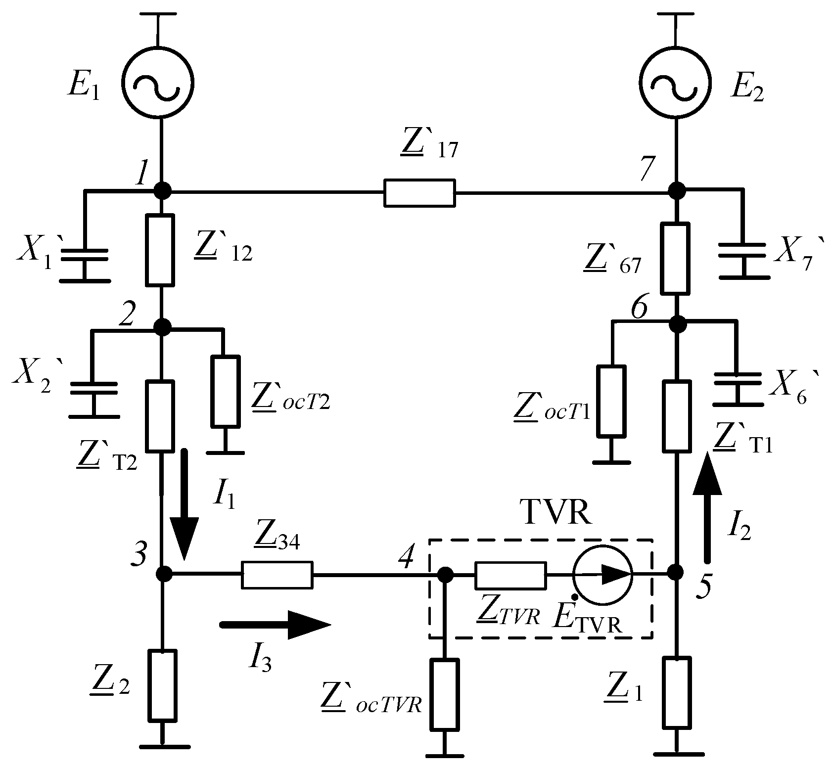
3. Calculation of the Steady-State Network Condition

The steady-state DN condition was calculated according to the proposed algorithm (Figure 2).

3.1. Assumptions

−

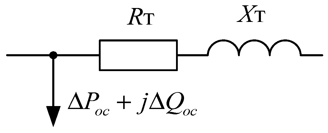
Two-winding transformers with U_HV.nom < 220 kV are represented by the following equivalent circuit (Figure 3) [19]:

−

The voltage regulator is characterized by an impedance introduced by series and shunt transformers, and a voltage source, which introduces an additional voltage into the line (Figure 4):

−

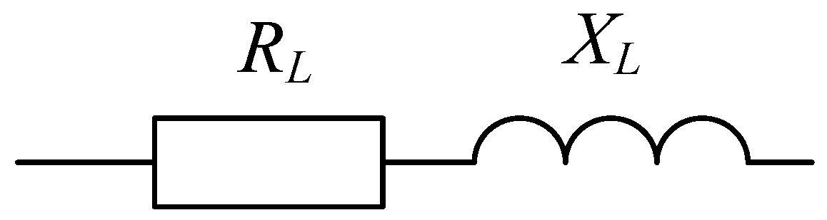
The equivalent circuit for the 110 kV transmission line (Figure 5) [19] is:

−

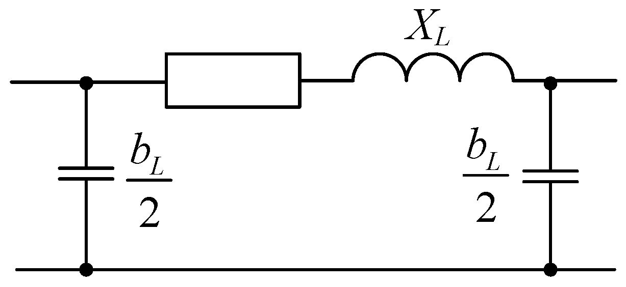
For overhead (OHL) and cable (CL) 10 kV lines, the admittance is not taken into account. The equivalent circuit in this case (Figure 6) is:

3.2. Equivalent Circuit

The calculated equivalent circuit for a network with a TVR is shown in Figure 7. It contains 8 nodes and 18 branches.

3.3. Parameters of Equivalent Circuit Elements

The calculated parameters of the power transmission lines are shown in

Table 1. Power transmission lines data.

Resistance, Ohm	Length, km	Wire Type	Specific Resistance, Ohm/km	Specific Inductive Reactance, Ohm/km	Specific Susceptance b0, S/km·10−6
Z12 = 10.55 + j11.1	25	ACSR 70/11	0.422	0.444	2.547
Z17 = 23.21 + j24.42	55	ACSR 70/11	0.422	0.444	2.547
Z67 = 29.54 + j31.08	70	ACSR 70/11	0.422	0.444	2.547
Z34 = 3.01 + j4.01	10	ACSR 95/16	0.301	0.401	–

, and the load data are presented in

Table 2. Load data.

Load	S, kVA	P, kW	Q, kvar	cosφ	Zph, Ohm
S12	5488	5268	1537	0.96	17.493 + j5.102
S21	4952	4605	1820	0.93	18.782 + j7.423

.

The TVR parameters are as follows:

−

Network voltage U_L = 10 kV ± 10%;

−

Phase angle between the output and input voltage θ = ±5°;

−

Range of output voltage amplitude relative to the input voltage amplitude regulation D = ±10%;

−

Load power 1800 kVA.

−

Load current I_L = 104 A.

3.4. Calculation of Transformers Parameters

Table 3. Transformers data.

Transformer Type	Snom, kVA	UHV, V	ULV, V	Ioc, %	Usc, %
Distribution transformer	16,000	110,000	10,000	0.7	10.5
Shunt (three-phase)	300	10,000	500/330/330	2.2	6.0
Serial (single-phase)	80	765	765	1.5	4.2

shows the main parameters of transformers. According to the catalog [20], the short-circuit impedance of the transformer referred to the primary side is Z`t = 4.38 + j86.7 Ohm.

The short-circuit impedance referred to the secondary side 10 kV is:

$${\underset{\_}{\mathrm{Z}`}}_{\mathrm{T}}=\frac{{\underset{\_}{\mathrm{Z}}}_{\mathrm{T}}}{{\mathrm{K}}^2}=\frac{4.38+\mathrm{j}86.7}{{11}^2}=0.036+\mathrm{j}0.717 \mathrm{Ohm},$$

(5)

where K is the transformation ratio.

The referred impedance of the magnetization branch is:

$${\underset{\_}{\mathrm{Z}`}}_{\mathrm{ocT}}=\frac{{\underset{\_}{\mathrm{Z}}}_{\mathrm{ocT}}}{{\mathrm{K}}^2}=\frac{5.34·{10}^4+\mathrm{j}3.15·{10}^4}{{11}^2}=441.7+\mathrm{j}2604 \mathrm{Ohm}.$$

(6)

To determine the TVR impedance Z_TVR, the equivalent circuit of one TVR phase under the combined control mode is considered. It is assumed that there is no pulse-phase regulation to simplify the calculations. In this case, the regulation steps of voltage magnitude and phase angle control modules are completely included in the work during the period of the supply voltage. In this mode, the maximum possible Z_TVR is included into the line (Figure 8).

For the presented equivalent circuit (Figure 8):

Z`<sub>sh</sub> = Z<sub>sc</sub>`_TM2 + Z_sc`<sub>TM11</sub> + Z<sub>sc</sub>`_TM12,

(7)

where Z`_sh is the shunt transformer impedance, referred to the voltage of the series transformer primary winding. According to the manufacturer’s data, the short-circuit impedance of the shunt and series transformers referred to the secondary side is:

Z`_sh = 1.103 + j0.679 Ohm;

(8)

Z`_se = 0.531 + j0.708 Ohm.

(9)

Taking into account that the transformation ratio of the series transformer K = 1, the maximum value of the impedance introduced by the TVR into the line is:

Z_TVR = Z`<sub>sh</sub> + Z`_se = 1.634 + j1.1387 Ohm;

(10)

Z_TVR = 2.143 Ohm.

(11)

The no-load losses of the TVR transformer equipment are made up of the no-load losses of the shunt and series transformers:

$${\underset{\_}{\mathrm{Z}`}}_{\mathrm{ocTVR}}=75454+\mathrm{j}41281 \mathrm{Ohm}.$$

(12)

3.5. Referring Line Parameters to Base Voltage

The network parameters are referred to the base voltage U_L = 10 kV to simplify the calculations. The parameters’ recalculation is carried out through the square of the transformation ratio of the transformer, which connects networks of different rated voltages.

Thus, the parameters of the 110 kV line referred to a voltage of 10 kV are:

$${\underset{\_}{\mathrm{Z}`}}_{17}=\frac{{\underset{\_}{\mathrm{Z}}}_{17}}{{\mathrm{K}}^2}=\frac{23.21+\mathrm{j}24.42}{{11}^2}=0.192+\mathrm{j}0.202 \mathrm{Ohm};$$

(13)

$${\underset{\_}{\mathrm{Z}`}}_{12}=\frac{{\underset{\_}{\mathrm{Z}}}_{12}}{{\mathrm{K}}^2}=\frac{10.55+\mathrm{j}11.1}{{11}^2}=0.087+\mathrm{j}0.092 \mathrm{Ohm};$$

(14)

$${\underset{\_}{\mathrm{Z}`}}_{67}=\frac{{\underset{\_}{\mathrm{Z}}}_{67}}{{\mathrm{K}}^2}=\frac{29.54+\mathrm{j}31.08}{{11}^2}=0.244+\mathrm{j}0.257 \mathrm{Ohm},$$

(15)

where K is the transformation ratio of the distribution transformer.

The susceptance b at the end of the 110 kV line [19] is:

$${\mathrm{b}}_{17}={\mathrm{b}}_{0}55\frac{1}{2}=2.547·{10}^{-6}·55\frac{1}{2}=7·{10}^{-5} \mathrm{S};$$

(16)

$${\mathrm{b}}_{12}={\mathrm{b}}_{0}15\frac{1}{2}=2.547·{10}^{-6}·15\frac{1}{2}=1.91·{10}^{-5} \mathrm{S};$$

(17)

$${\mathrm{b}}_{67}={\mathrm{b}}_{0}70\frac{1}{2}=2.547·{10}^{-6}·70\frac{1}{2}=8.91·{10}^{-5} \mathrm{S}.$$

(18)

OHL reactive power in nodes 1, 2, 6, and 7 (Figure 7) are as follows:

$${\mathrm{Q}}_1={\mathrm{U}}_{\mathrm{OHL}}^2·{\mathrm{b}}_{17}+{\mathrm{U}}_{\mathrm{OHL}}^2·{\mathrm{b}}_{12}={110000}^2·7·{10}^{-5}+{110000}^2·1.91·{10}^{-5}=1.079 \mathrm{Mvar}.$$

(19)

$${\mathrm{Q}}_2={\mathrm{U}}_{\mathrm{OHL}}^2·{\mathrm{b}}_{12}={110000}^2·1.91·{10}^{-5}=0.231 \mathrm{Mvar}.$$

(20)

$${\mathrm{Q}}_6={\mathrm{U}}_{\mathrm{OHL}}^2·{\mathrm{b}}_{67}={110000}^2·8.914·{10}^{-5}=1.078 \mathrm{Mvar}.$$

(21)

$${\mathrm{Q}}_7={\mathrm{U}}_{\mathrm{OHL}}^2·{\mathrm{b}}_{17}+{\mathrm{U}}_{\mathrm{OHL}}^2·{\mathrm{b}}_{67}={110000}^2·7·{10}^{-5}+{110000}^2·8.914·{10}^{-5}=1.929 \mathrm{Mvar}.$$

(22)

The referred reactance corresponding to the OHL reactive power in nodes 1, 2, 6, and 7 (Figure 7) is:

$$\mathrm{X}{`}_1=-\mathrm{j}\frac{{\mathrm{U}}_{\mathrm{OHL}}{}^2}{{\mathrm{Q}}_1{\mathrm{K}}^2}=-\mathrm{j}92.708 \mathrm{Ohm};$$

(23)

$${\mathrm{X}}_2`=-\mathrm{j}\frac{{\mathrm{U}}_{\mathrm{OHL}}{}^2}{{\mathrm{Q}}_2{\mathrm{K}}^2}=-\mathrm{j}432.6 \mathrm{Ohm};$$

(24)

$$\mathrm{X}{`}_6=-\mathrm{j}\frac{{\mathrm{U}}_{\mathrm{OHL}}{}^2}{{\mathrm{Q}}_6{\mathrm{K}}^2}=-\mathrm{j}117.9 \mathrm{Ohm};$$

(25)

$$\mathrm{X}{`}_7=-\mathrm{j}\frac{{\mathrm{U}}_{\mathrm{OHL}}{}^2}{{\mathrm{Q}}_6{\mathrm{K}}^2}=-\mathrm{j}51.9 \mathrm{Ohm}.$$

(26)

3.6. Directed Graph

The calculated equivalent circuit (Figure 7) corresponds to the directed graph shown in Figure 9. An incidence matrix is compiled for it.

3.7. Incidence Matrix

The incidence matrix for the graph (Figure 9) is as follows:

$$A=\left[\begin{array}{cccccccccccccccccc}-1& 1& 1& 1& 0& 0& 0& 0& 0& 0& 0& 0& 0& 0& 0& 0& 0& 0\\ 0& 0& -1& 0& 1& 1& 1& 0& 0& 0& 0& 0& 0& 0& 0& 0& 0& 0\\ 0& 0& 0& 0& 0& -1& 0& 1& 1& 0& 0& 0& 0& 0& 0& 0& 0& 0\\ 0& 0& 0& 0& 0& 0& 0& 0& -1& 1& 1& 0& 0& 0& 0& 0& 0& 0\\ 0& 0& 0& 0& 0& 0& 0& 0& 0& 0& -1& 1& -1& 0& 0& 0& 0& 0\\ 0& 0& 0& 0& 0& 0& 0& 0& 0& 0& 0& 0& 1& 1& 1& -1& 0& 0\\ 0& 0& 0& -1& 0& 0& 0& 0& 0& 0& 0& 0& 0& 0& 0& 1& 1& -1\end{array}\right]$$

(27)

The obtained equations (Equations (1)–(27)) allow the main electrical quantities (currents, voltages, and powers) under voltage magnitude, phase angle, and combined TVR control modes to be determined. The calculation was carried out using the Mathcad program. As a result of the calculations, the dependences of the power, voltage, and current of the DN on the additional voltage were obtained. The calculations show that accounting for the transformers’ magnetization branches and the reactive power generated by 110 kV power transmission lines has a small effect on the currents and power flows transmission in the lines. Neglecting these parameters introduces an inaccuracy in the calculations of less than 0.5%. Thus, in further calculations, in order to reduce the number of equations, simplify the model, and reduce the simulation time, these parameters can be ignored.

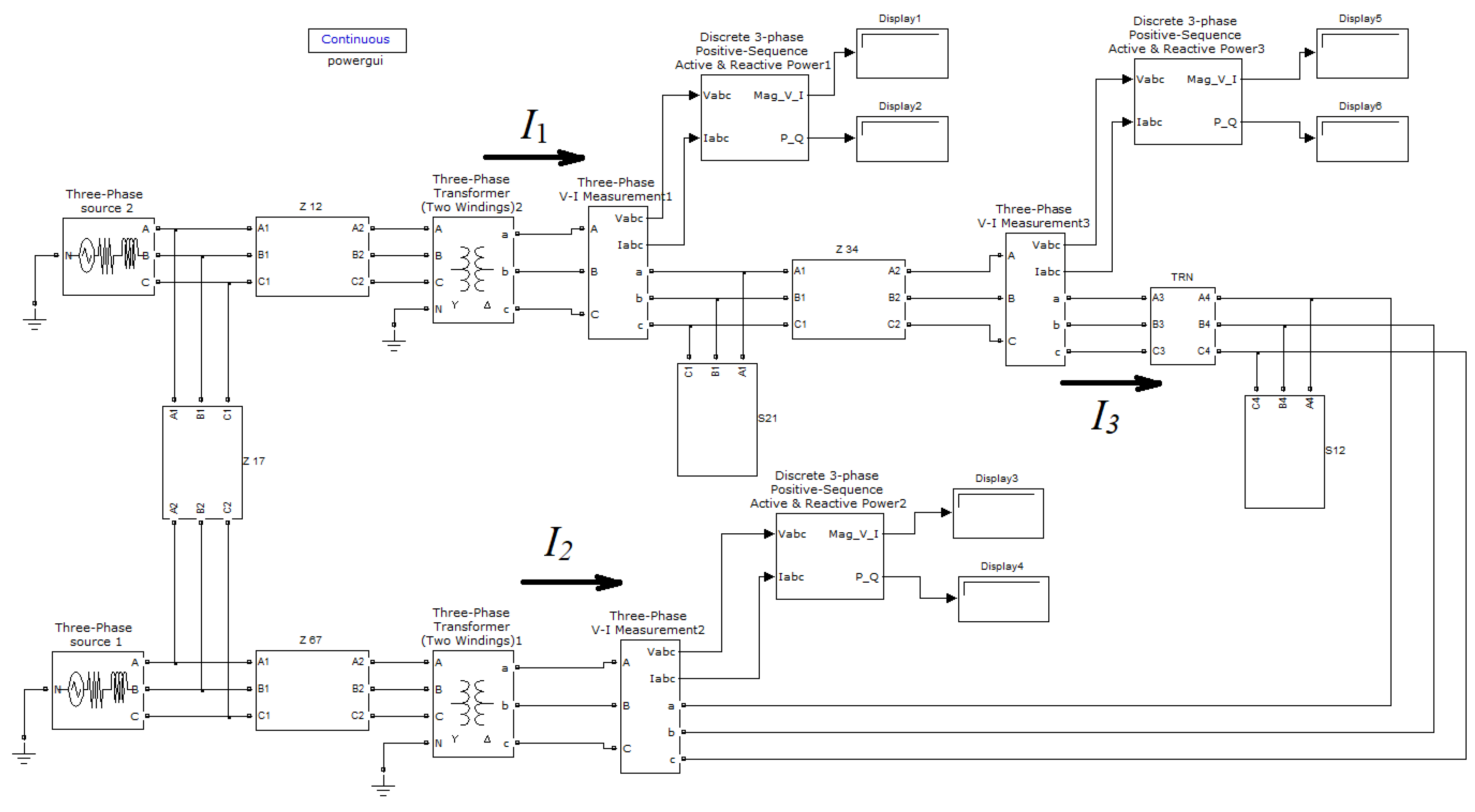
4. Simulation of the DN Operating Modes in Matlab Simulink

A simulation model was developed for the MV DN (Figure 10) in order to verify the analytical calculations obtained by the matrix-oriented method [21]. The model was developed in the MATLAB Simulink according to the equivalent circuit (Figure 7).

The simulated 10 kV DN is fed by the power system through two step-down substations SS 110/10 kV and contains 2 load nodes. When developing the model, the resistances of 110 kV overhead power transmission lines and 10 kV distribution power lines located between load nodes and the short-circuit impedance of transformers were taken into account.

The TVR model was made with Simulink blocks. When developing it, a modular principle of implementing the power circuit and control system was used. To implement vector control, the power circuit has series-connected voltage magnitude and phase angle control modules in a three-phase design. The voltage magnitude control module generates a voltage injected in-phase or anti-phase with the voltages of the 10 kV network. The phase angle control module generates a voltage injected with an angular relationship with respect to phase voltage that achieves the desired phase shift (advance or retard) without any change in magnitude.

5. Results and Discussion

The TVR efficiency is illustrated by the dependences of currents and powers on the TVR additional voltage, obtained by modeling in Simulink and the matrix-oriented method in Mathcad.

It has been established that the difference between the results of a computer simulation and analytical calculations is no more than 2% under voltage magnitude and phase angle control modes. This difference is due to the assumptions made when compiling an equivalent circuit for analytical calculations and the Simulink model. The analytical model does not take into account the voltage drops across the thyristors and the change in the TVR impedance introduced into the line under regulation. The transformers have been represented by a simplified equivalent circuit [22].

Figure 11 shows the graphs of current components I₁, I₂, and I₃ under voltage magnitude and phase angle control modes.

The step of the additional voltage of the voltage magnitude and phase angle control modules is ±600 V. It provides a range of voltage magnitude controls of ±10.4% and phase angle controls of ±5.9°. It can be seen from the dependencies (Figure 11) that the control of the real and reactive components of the currents occurs both under voltage magnitude and phase angle control modes.

The largest range of current regulation is observed under the combined control mode. Figure 12 shows the dependences of RMS currents I₁, I_2, and I₃ with different regulating methods of the TVR output voltage. The presented graphs allow the determination of the current of the considered DN parts under the voltage magnitude, phase angle, and combined control modes.

The use of the TVR allows loading the lines with currents I₁ and I₂ (Figure 7) in proportion to the power transmission line transfer capability in the selected range of magnitude and phase of the additional voltage vector. In this case, the currents I₁ and I₂ will be equal when using overhead lines with the same characteristics. The condition I₁ = I₂ can be fulfilled at different proportions of the voltage of the voltage magnitude and phase angle control modules (Figure 13). I₁ and I₂ surfaces determine all possible values of these currents under combined control modes at the ±600 V range of additional voltage variation. The presented dependencies were obtained with constant load parameters.

The DN power flow transmission parameters have been calculated (Figure 7) for voltage magnitude, phase angle, and combined control modes. Figure 14 shows the ranges of real and reactive power changes of power lines with currents I₁, I₂, and I₃ under the combined control mode.

It has been established that in all ranges of the combined control mode, the real power flows P₁ and P₂ do not change their sign. Consequently, the direction of real power in the DN containing distribution transformers (Figure 7) is unchanged and is directed from the high-voltage network to the load.

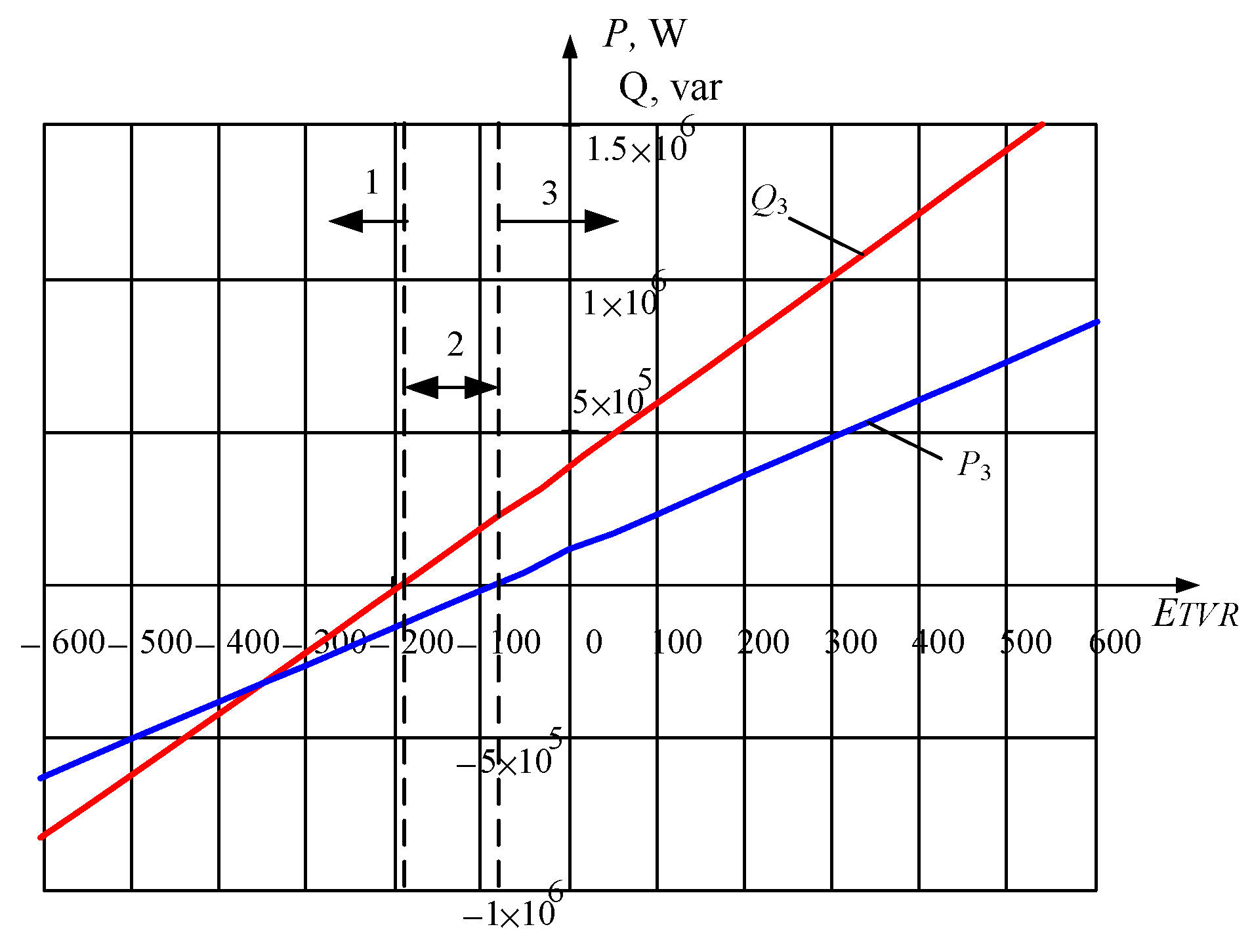
The conducted studies have shown that the direction and value of real and reactive power transmission between substations SS1 and SS2 (Figure 1) depend significantly on the regulation step of voltage magnitude and phase angle control modules. Figure 15 shows an example of the dependences of real and reactive power flows transmission between substations SS1 and SS2 on the additional voltage under the voltage magnitude control mode.

There are the following modes of power transmission under the combined control mode:

1. The mode corresponding to negative values of real P₃ and reactive Q₃ powers. Their flow is directed through the TVR from SS1 to SS2 (Figure 1).

2. The mode corresponding to the negative value of real power P₃ and the positive value of reactive power Q₃. The real power flow is directed from SS1 to SS2 through the TVR, and the reactive power flow is directed from SS2 to SS1.

3. The mode corresponding to the positive values of real P₃ and reactive Q₃ powers. Their flow is directed through the TVR from SS2 to SS1.

4. For the mode P₃ = 0, there is no real power flow between SS1 and SS2.

5. For the mode Q₃ = 0, there is no reactive power flow between SS1 and SS2.

6. For the mode of simultaneous implementation of the conditions P₃ = 0 and Q₃ = 0 (Figure 16), there are no real and reactive power flows between SS1 and SS2 at the point I₃ = 0.

6. Conclusions

The use of semiconductor devices for automatic voltage regulation and real and reactive power flows control is one of the ways to increase the efficiency of medium-voltage distribution networks. One of such devices is the thyristor voltage regulator.

The developed device allows vector voltage regulation to be carried out (i.e., changing the voltage vector in magnitude and phase). The article presents the results of the study of steady-state conditions of the distribution network with a TVR. Power and current dependencies are obtained from the additional voltage of voltage magnitude, phase angle, and combined control.

The studies allowed the determination of the possibility of providing with the TVR the optimal flow transmission of real and reactive power over the power transmission lines in proportion to their transfer capability when the load and power factor change. The determination of parameters of these modes is necessary to create and configure an efficient TVR control system.

The results of the conducted studies can be used in the design and reconstruction of medium-voltage distribution networks using the TVR, which provide optimal current and power transmission modes. The TVR in distribution networks reduces power and voltage losses, increases transfer capability, and reduces the cost of transmitted electricity.