Author Contributions
Conceptualization, D.N., C.G., J.W. and C.F.; methodology, D.N. and J.S.; software, D.N. and J.S.; validation, D.N. and J.S.; investigation, D.N., J.S. and J.W.; resources, J.W.; writing—original draft preparation, D.N.; visualization, D.N. and J.S.; supervision, A.M. and C.F.; project administration, A.M., C.G. and C.B.; funding acquisition, A.M., C.G. and C.B. All authors have read and agreed to the published version of the manuscript.
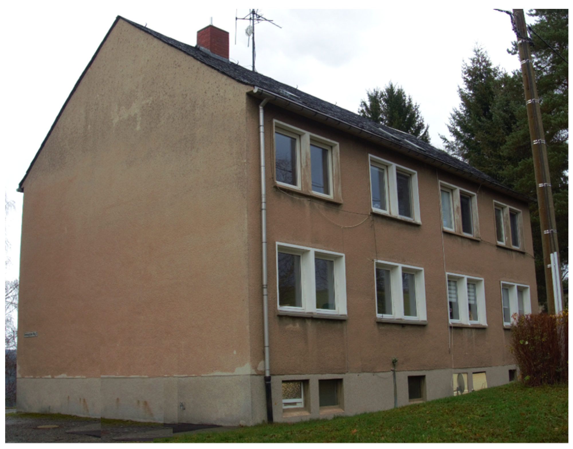
Figure 1.
West-side view of the field trial building.
Figure 1.
West-side view of the field trial building.
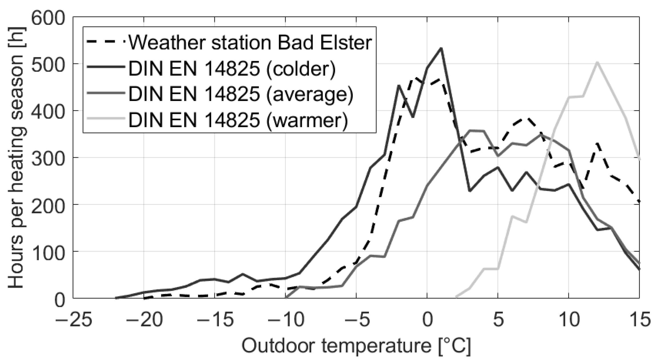
Figure 2.
Outdoor temperature distribution of the DWD weather station Bad Elster from 28 June 2020 to 27 June 2021 compared to DIN EN 14825 [
23].
Figure 2.
Outdoor temperature distribution of the DWD weather station Bad Elster from 28 June 2020 to 27 June 2021 compared to DIN EN 14825 [
23].
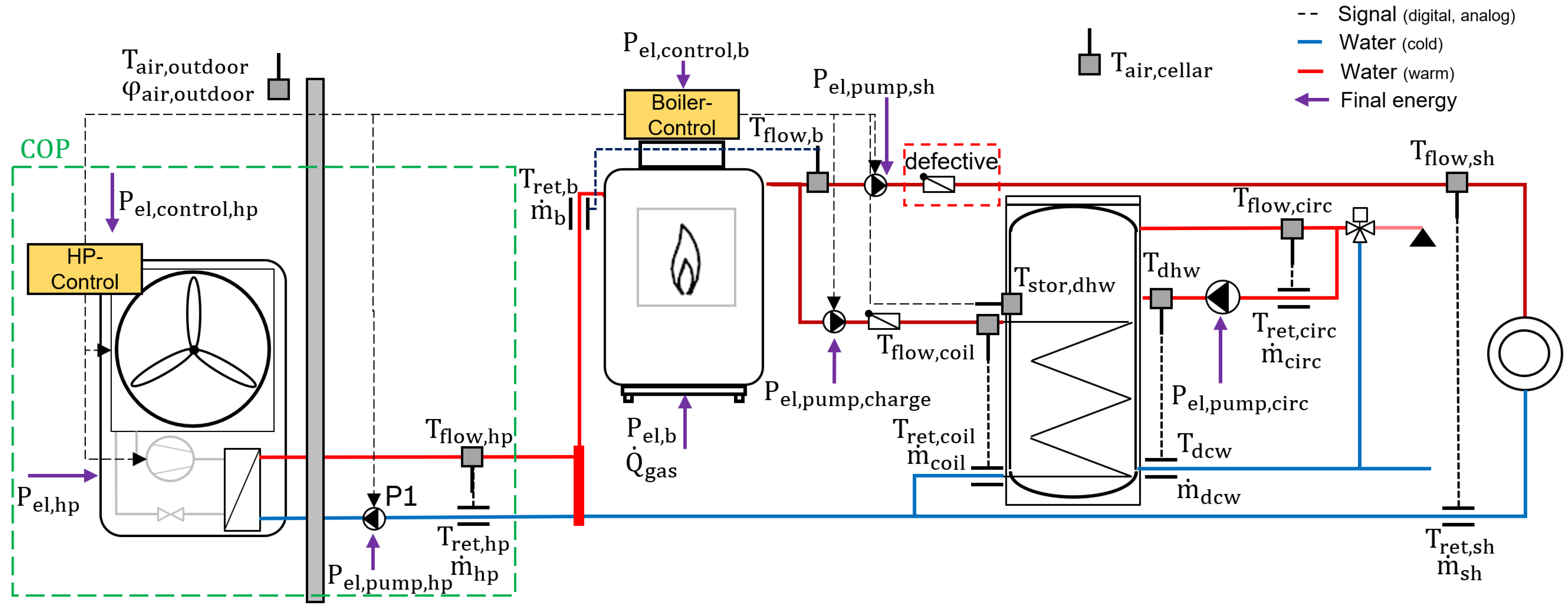
Figure 3.
Hydraulic and control schematic of the field trial with measurement positions and defective SH nonreturn valve.
Figure 3.
Hydraulic and control schematic of the field trial with measurement positions and defective SH nonreturn valve.
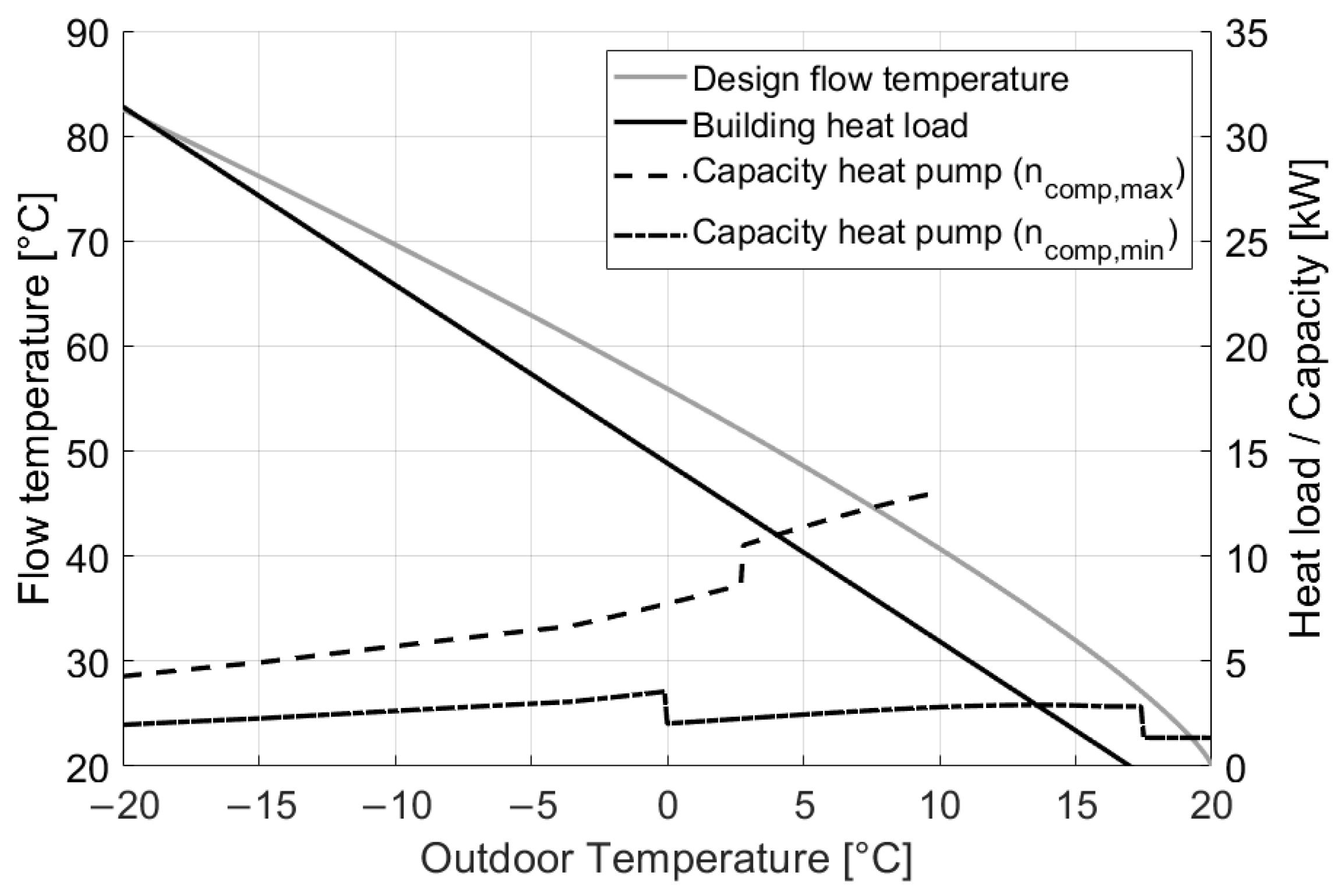
Figure 4.
WCC flow temperature and heat load of the building with the thermal capacity of the heat pump with maximum and minimum compressor frequency.
Figure 4.
WCC flow temperature and heat load of the building with the thermal capacity of the heat pump with maximum and minimum compressor frequency.
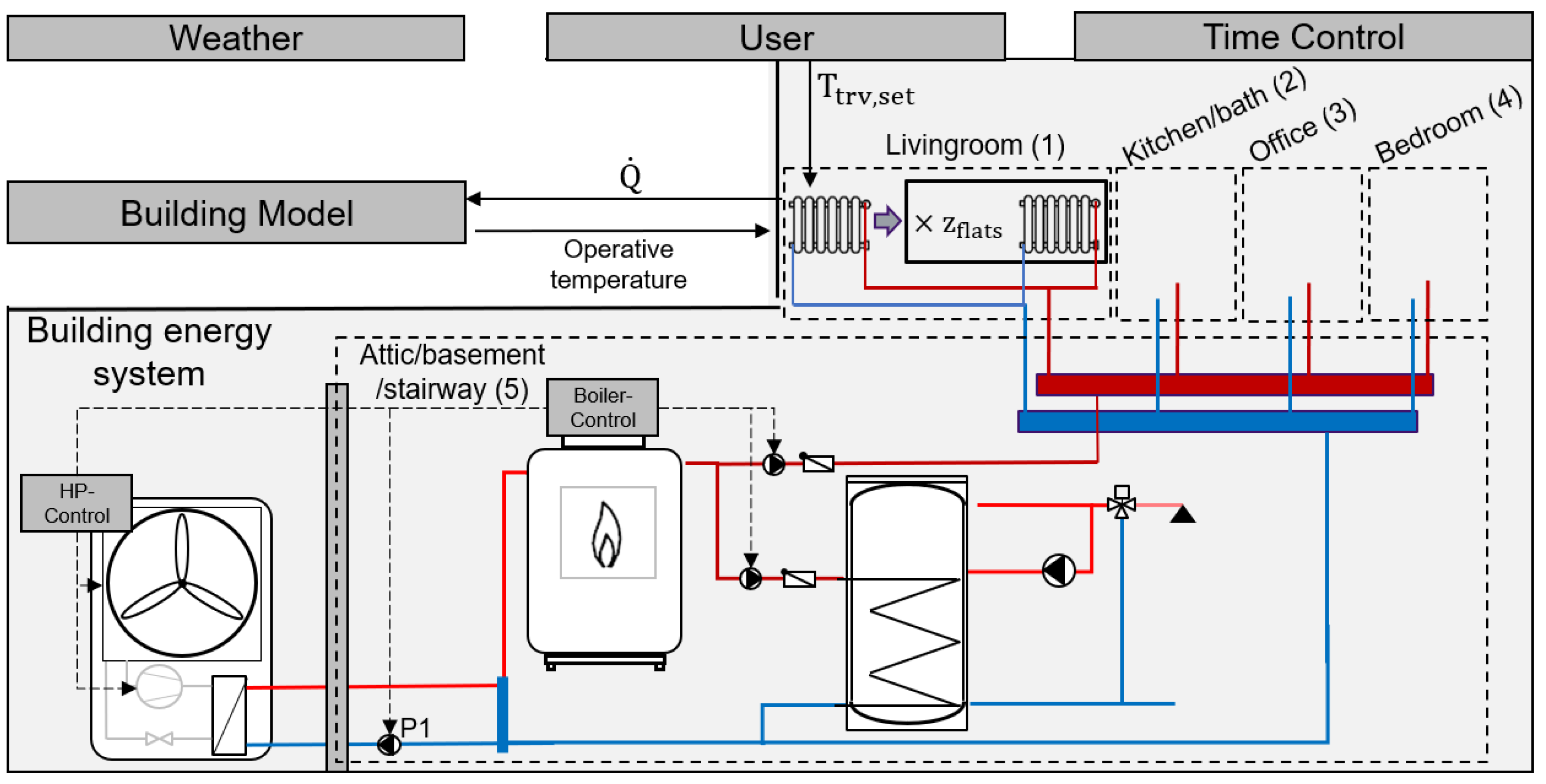
Figure 5.
Building simulation model schematic.
Figure 5.
Building simulation model schematic.
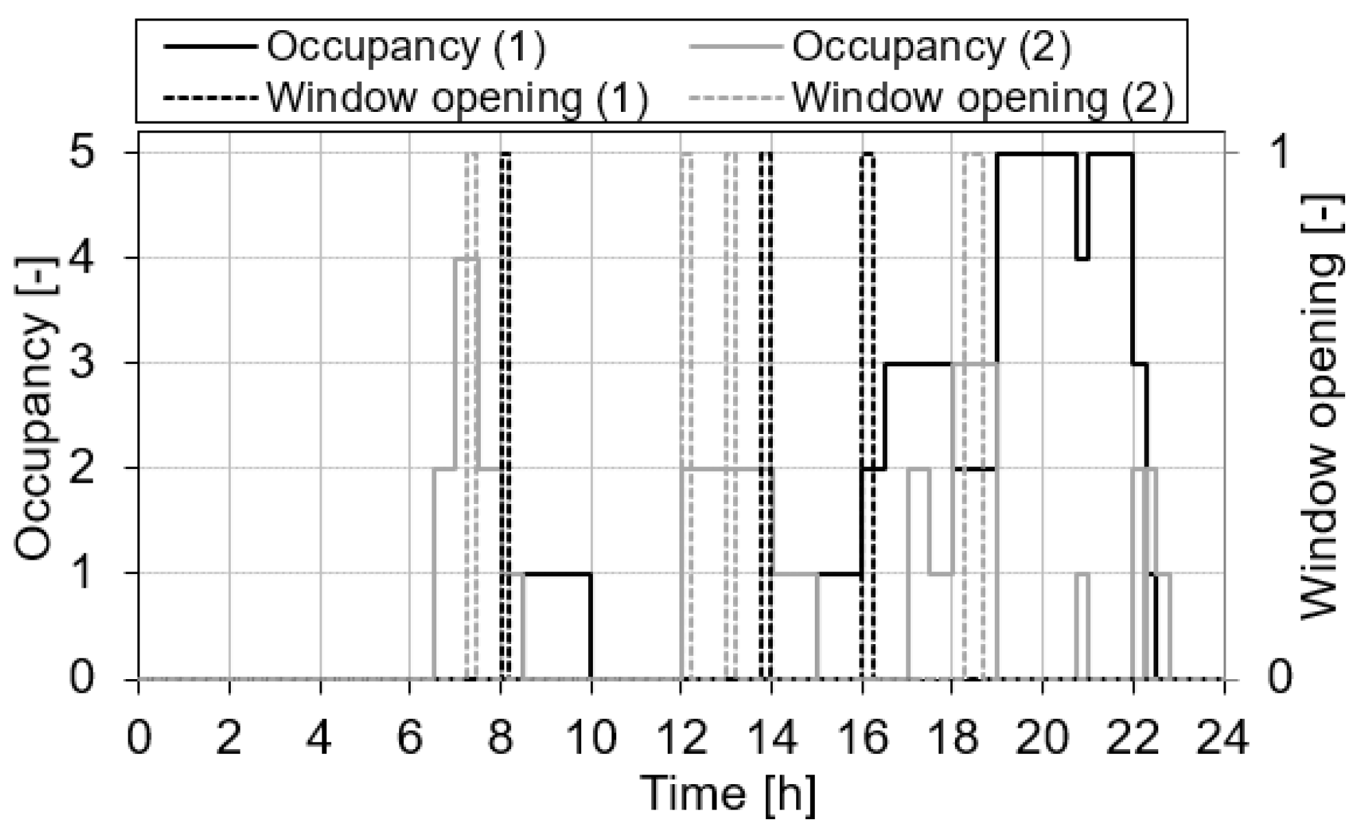
Figure 6.
Occupancy and ventilation profile of the living room (1) and the kitchen/bath (2).
Figure 6.
Occupancy and ventilation profile of the living room (1) and the kitchen/bath (2).
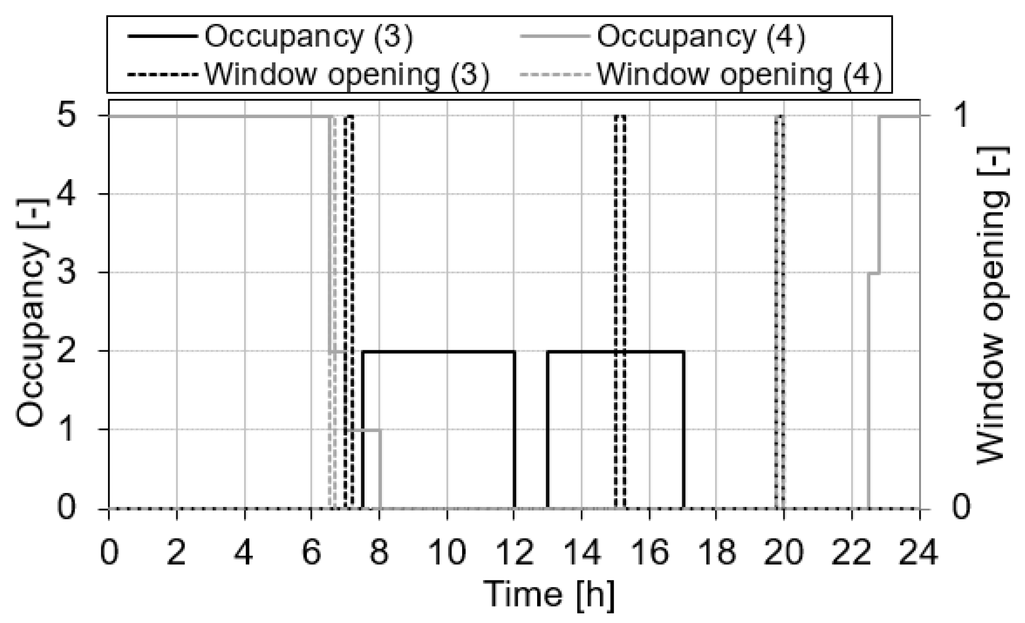
Figure 7.
Occupancy and ventilation profile of the office room (3) and the bedroom (4).
Figure 7.
Occupancy and ventilation profile of the office room (3) and the bedroom (4).
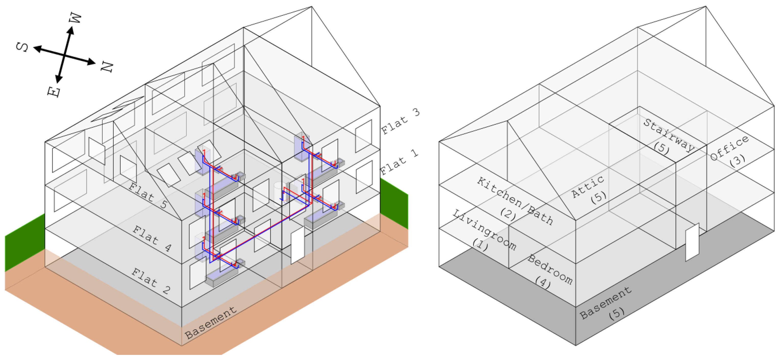
Figure 8.
Schematic building structure (left) and simulation model representation (right).
Figure 8.
Schematic building structure (left) and simulation model representation (right).
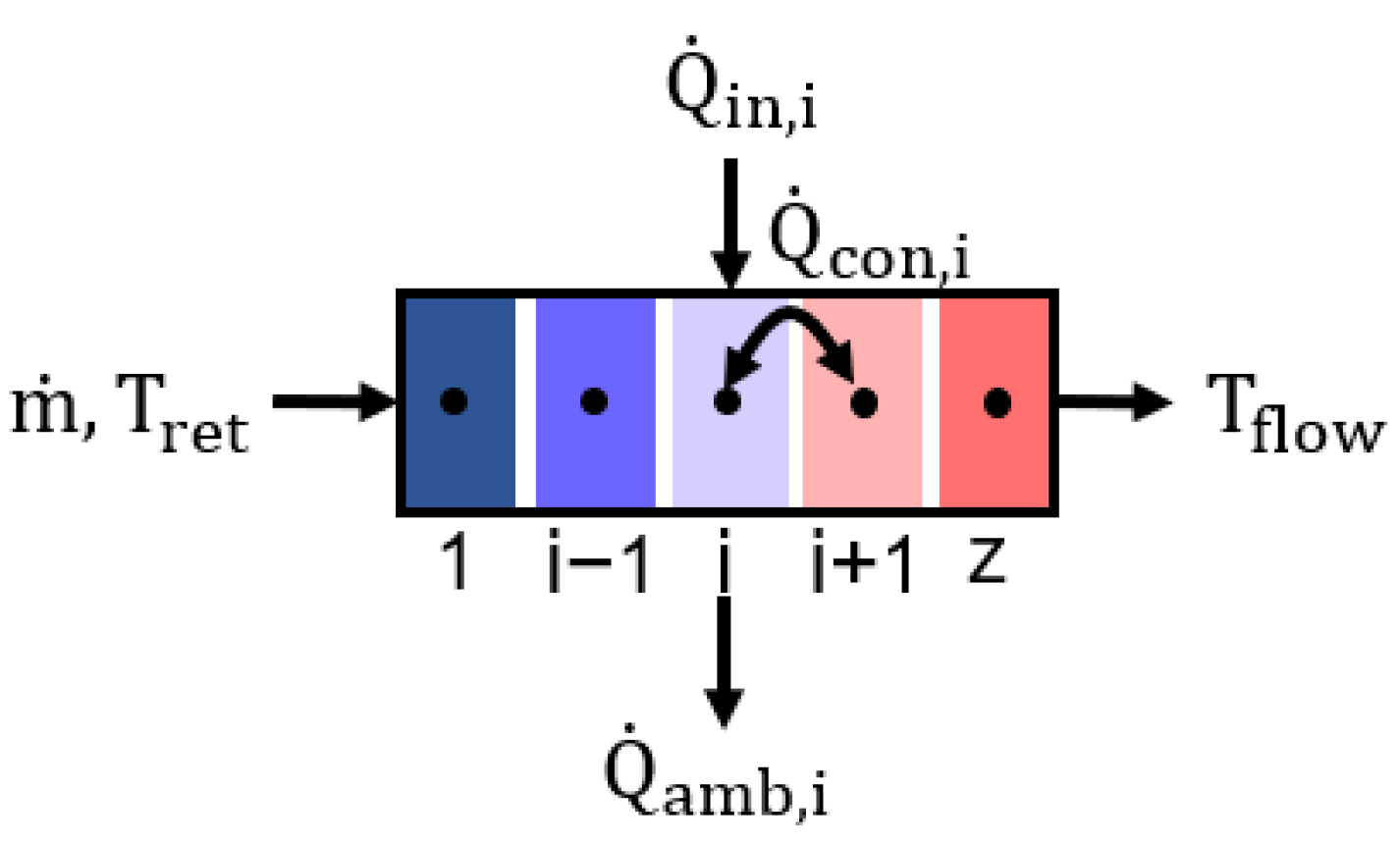
Figure 9.
Schematic heat balance of the 1-D capacity model.
Figure 9.
Schematic heat balance of the 1-D capacity model.
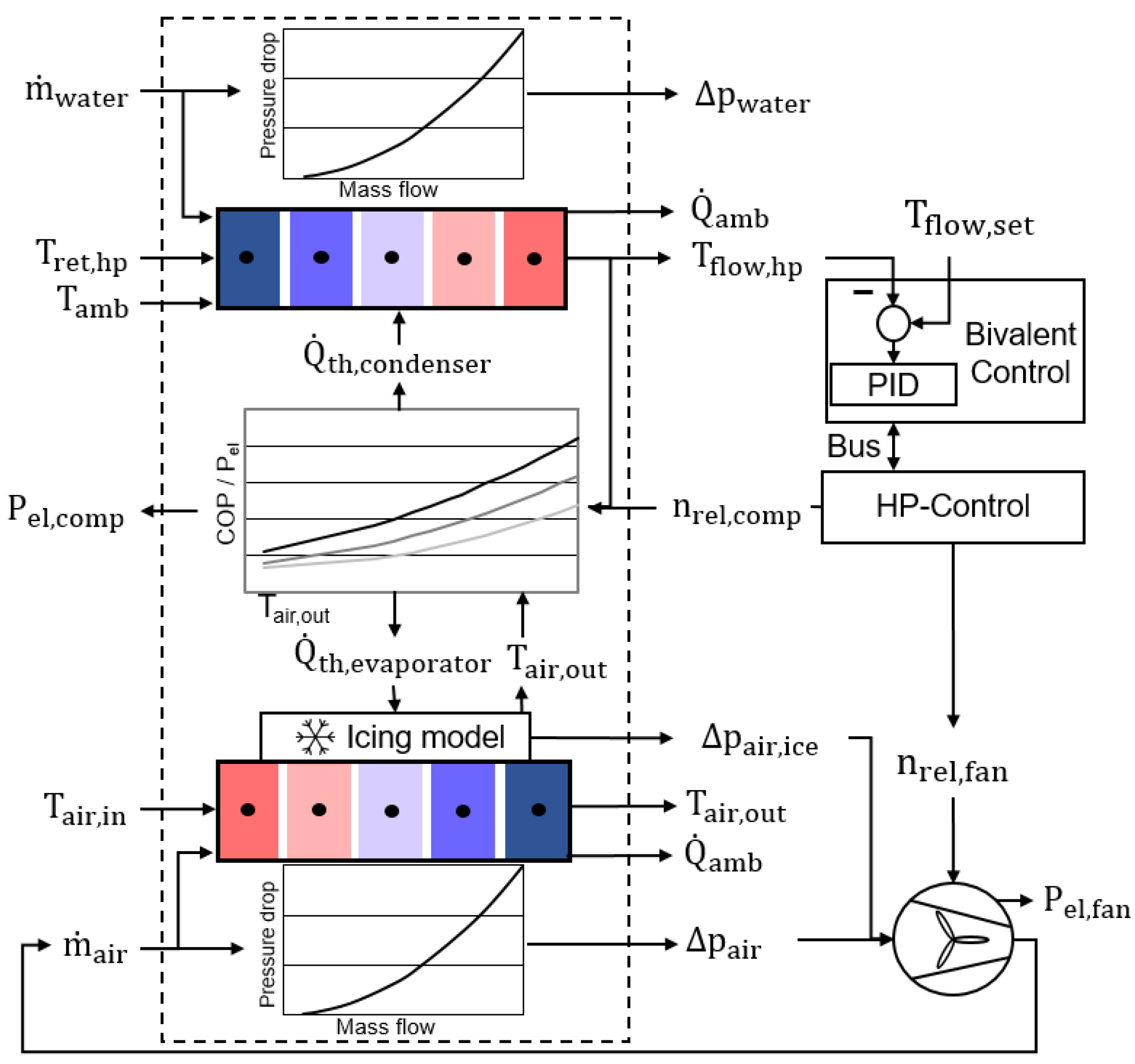
Figure 10.
Thermohydraulic heat pump model with curve-based efficiency model and controller scheme.
Figure 10.
Thermohydraulic heat pump model with curve-based efficiency model and controller scheme.
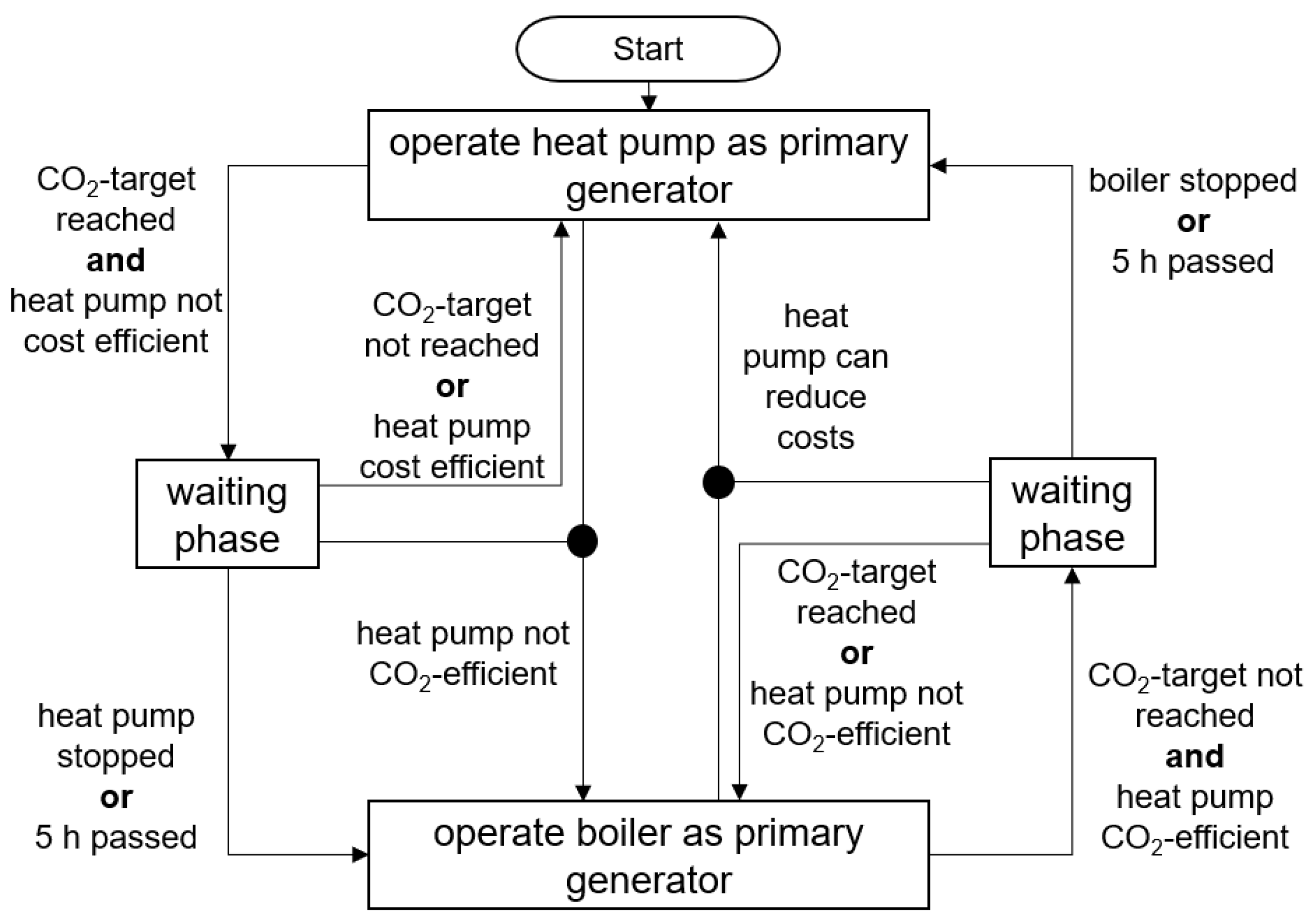
Figure 11.
Algorithm scheme to reach defined specific CO2 emission.
Figure 11.
Algorithm scheme to reach defined specific CO2 emission.
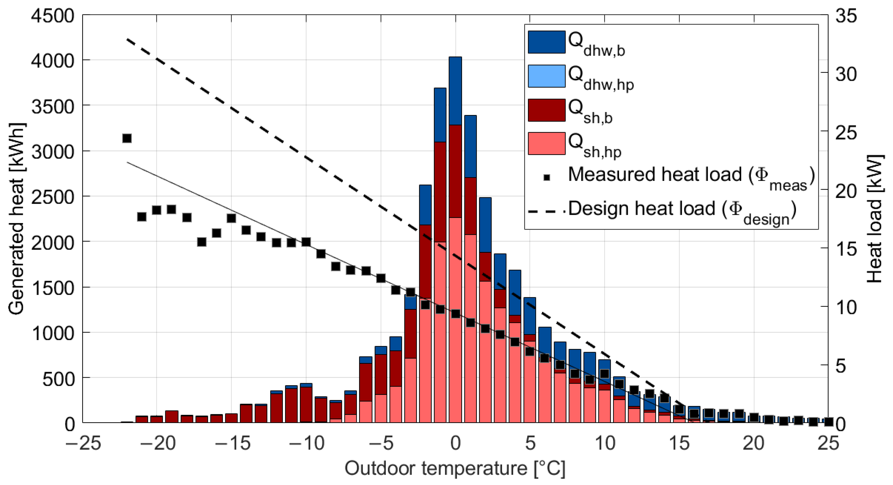
Figure 12.
Provided heat from heat pump and boiler with the calculated and measured mean building heat load.
Figure 12.
Provided heat from heat pump and boiler with the calculated and measured mean building heat load.
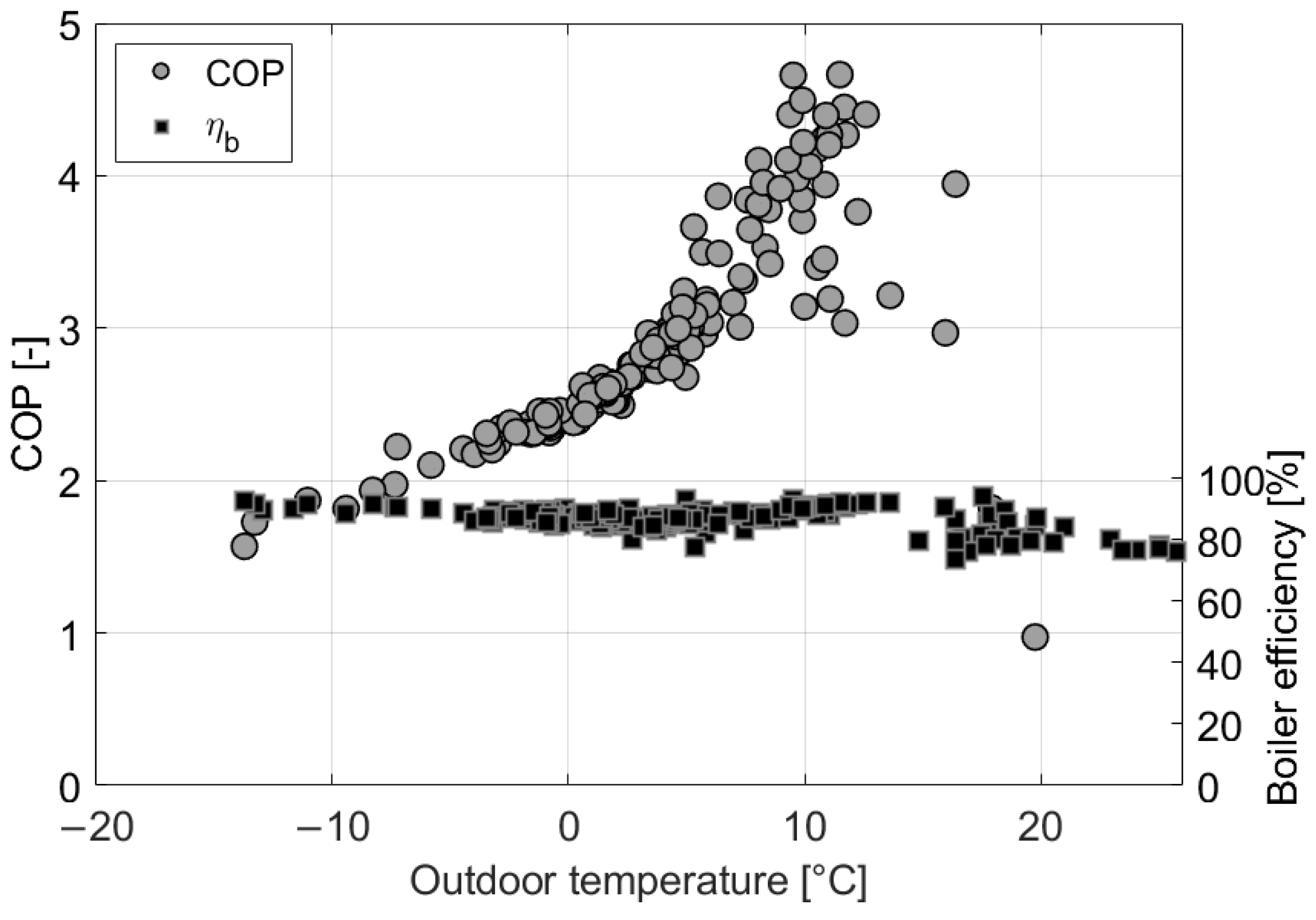
Figure 13.
Daily COP and boiler efficiency (axis scaled with the ratio of the CO2 emission factors).
Figure 13.
Daily COP and boiler efficiency (axis scaled with the ratio of the CO2 emission factors).
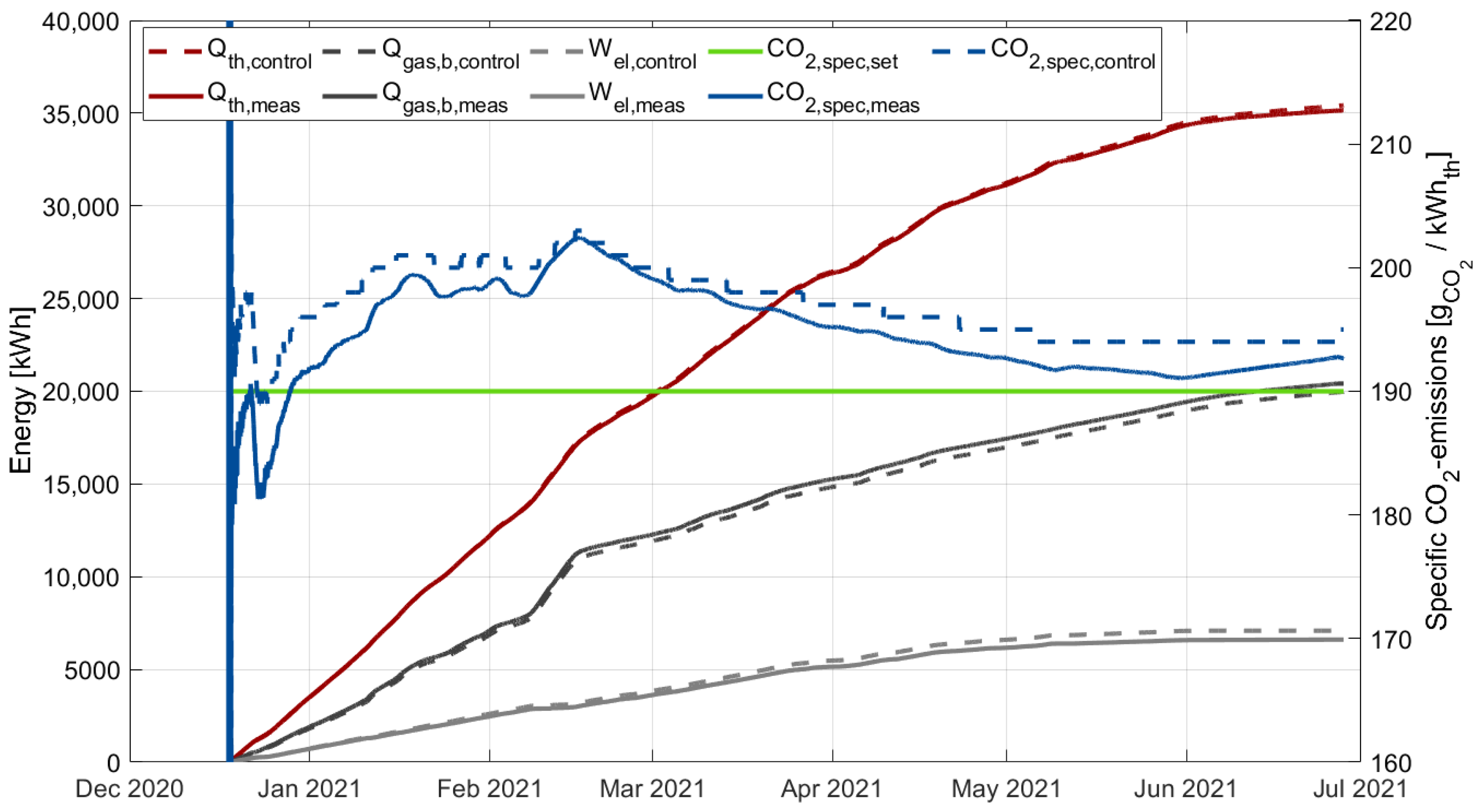
Figure 14.
Comparison of measured and internally calculated provided heat and used final energy of both heat generators and respective specific CO2 emission with corresponding set point.
Figure 14.
Comparison of measured and internally calculated provided heat and used final energy of both heat generators and respective specific CO2 emission with corresponding set point.
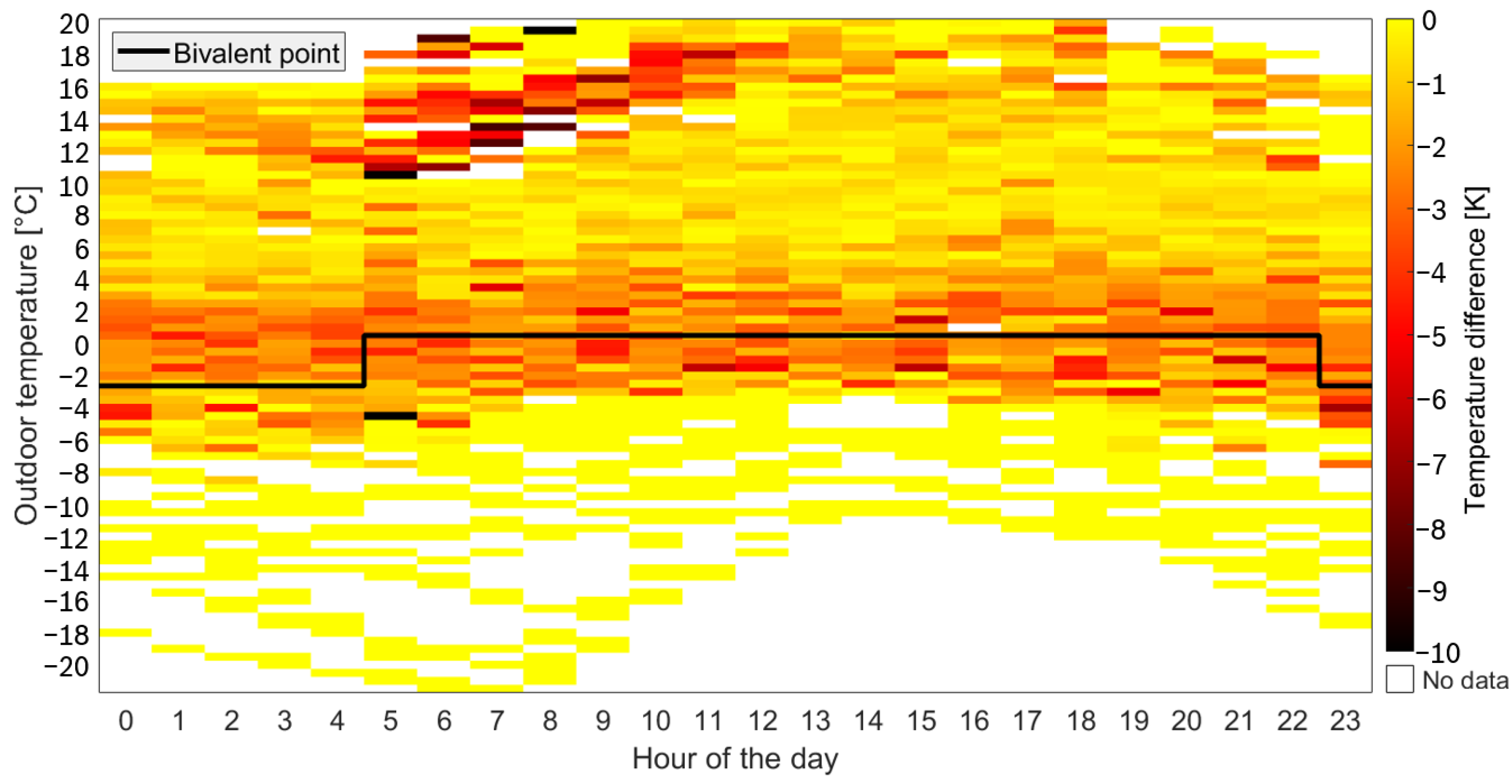
Figure 15.
Negative temperature differences of 15 min periods in dependency of the outdoor temperature and time of the day with bivalent point.
Figure 15.
Negative temperature differences of 15 min periods in dependency of the outdoor temperature and time of the day with bivalent point.
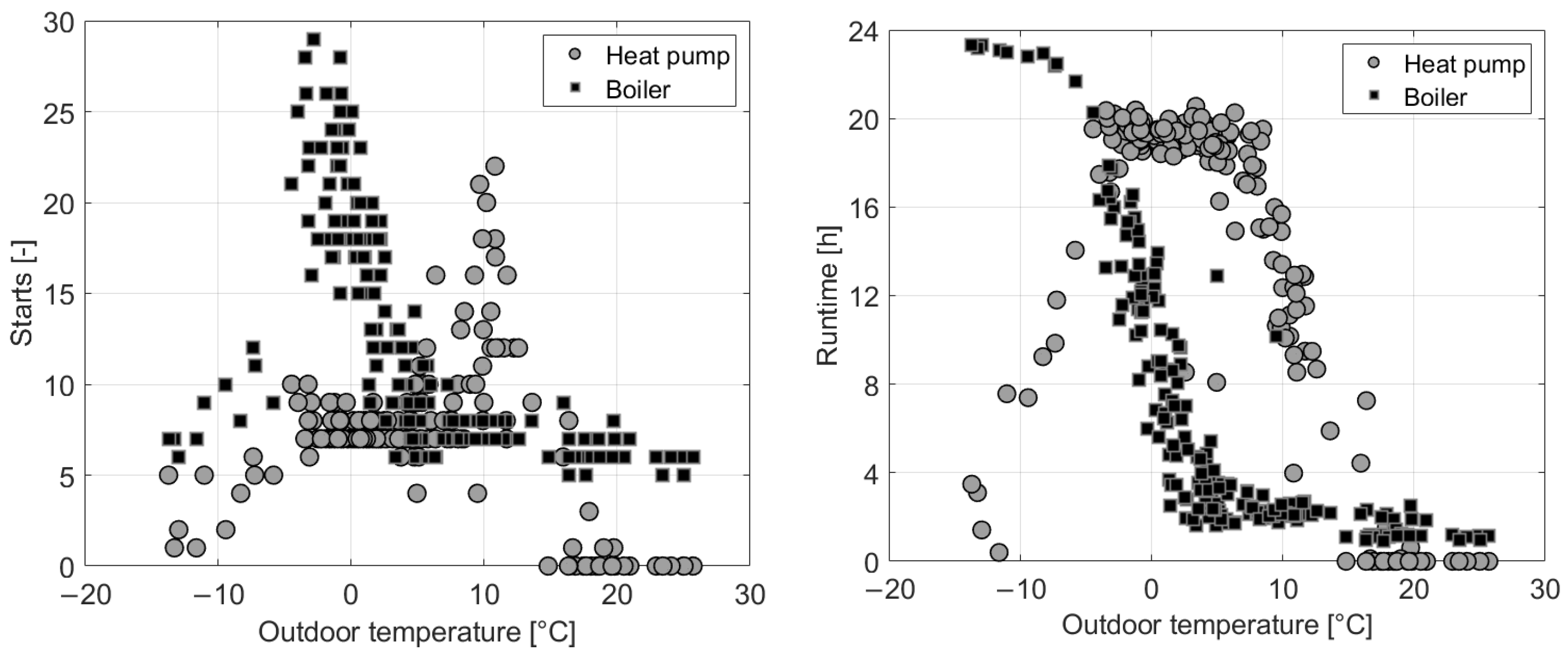
Figure 16.
Number of daily starts (left) and runtime (right) of the heat pump and boiler.
Figure 16.
Number of daily starts (left) and runtime (right) of the heat pump and boiler.
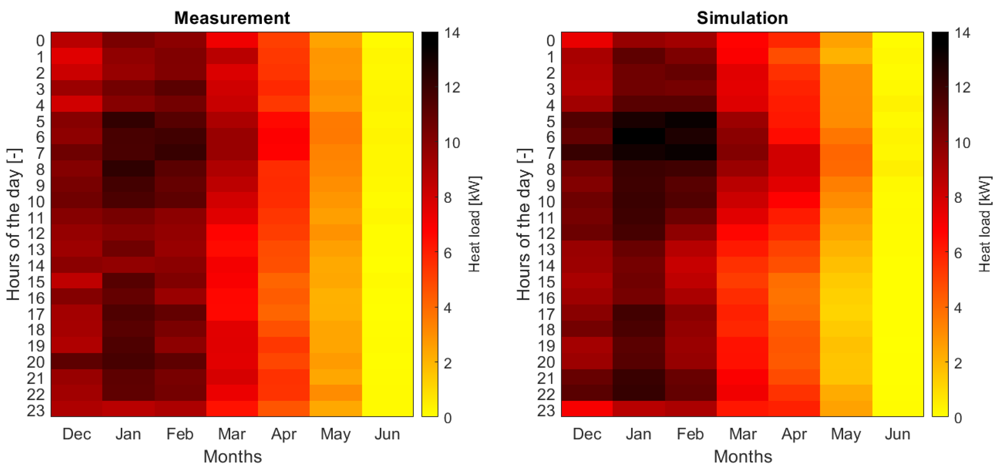
Figure 17.
Measured (left) and simulated (right) mean space heating demand for the hours of the day of all months.
Figure 17.
Measured (left) and simulated (right) mean space heating demand for the hours of the day of all months.
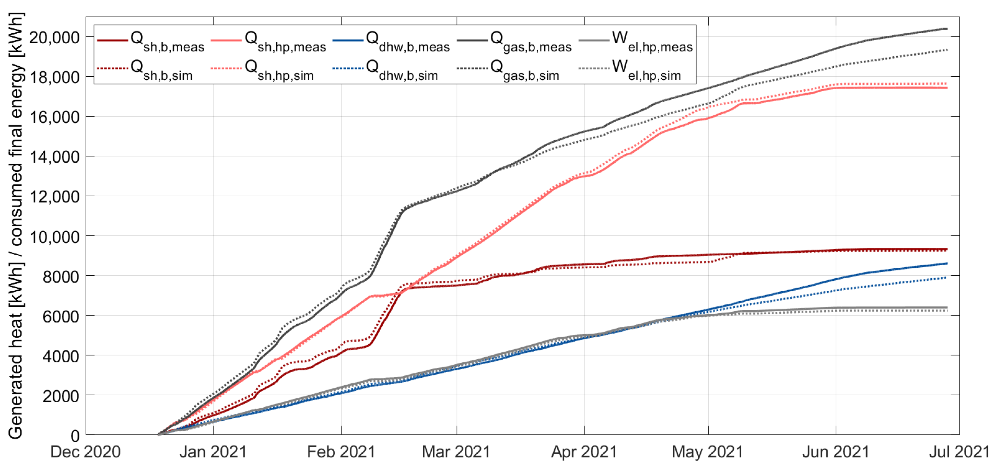
Figure 18.
Comparison of measured and simulated provided heat for space heating and domestic hot water preparation and used final energy of both heat generators.
Figure 18.
Comparison of measured and simulated provided heat for space heating and domestic hot water preparation and used final energy of both heat generators.
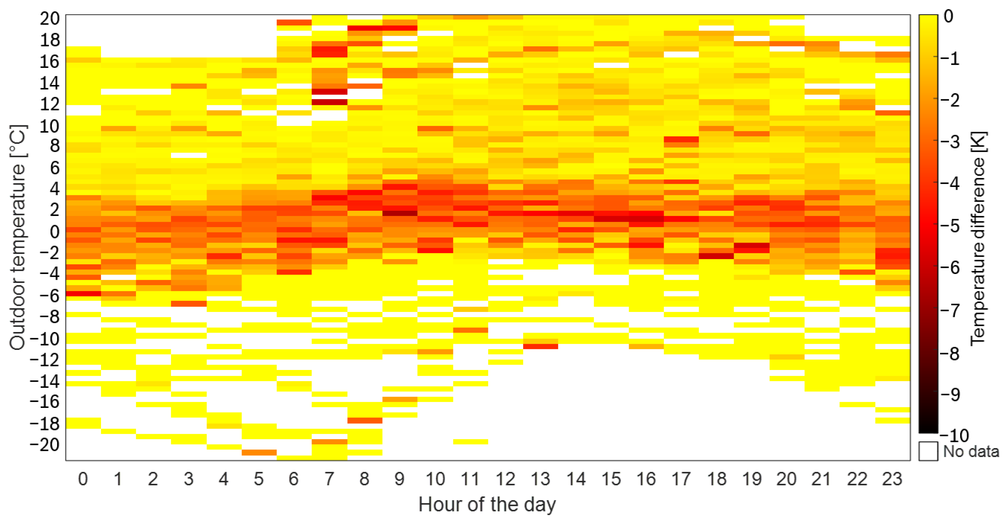
Figure 19.
Simulated negative temperature differences of 15-min periods in dependency of the outdoor temperature and time of the day.
Figure 19.
Simulated negative temperature differences of 15-min periods in dependency of the outdoor temperature and time of the day.
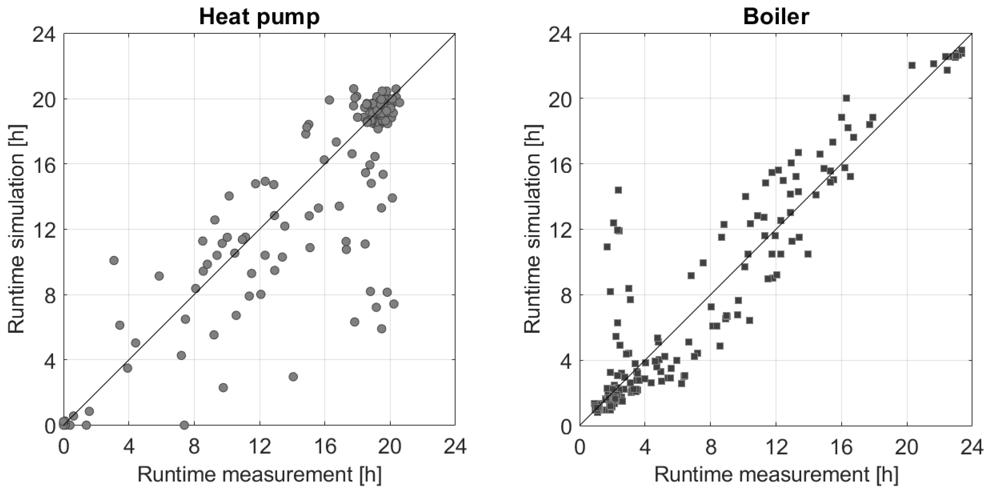
Figure 20.
Daily runtime of the heat pump (left) and the boiler (right) in simulation and measurement.
Figure 20.
Daily runtime of the heat pump (left) and the boiler (right) in simulation and measurement.
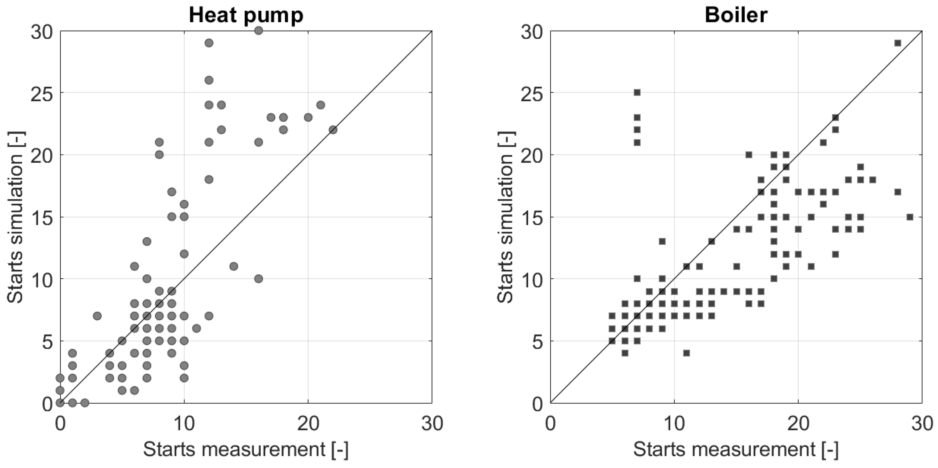
Figure 21.
Daily number of starts of the heat pump (left) and the boiler (right) in simulation and measurement.
Figure 21.
Daily number of starts of the heat pump (left) and the boiler (right) in simulation and measurement.
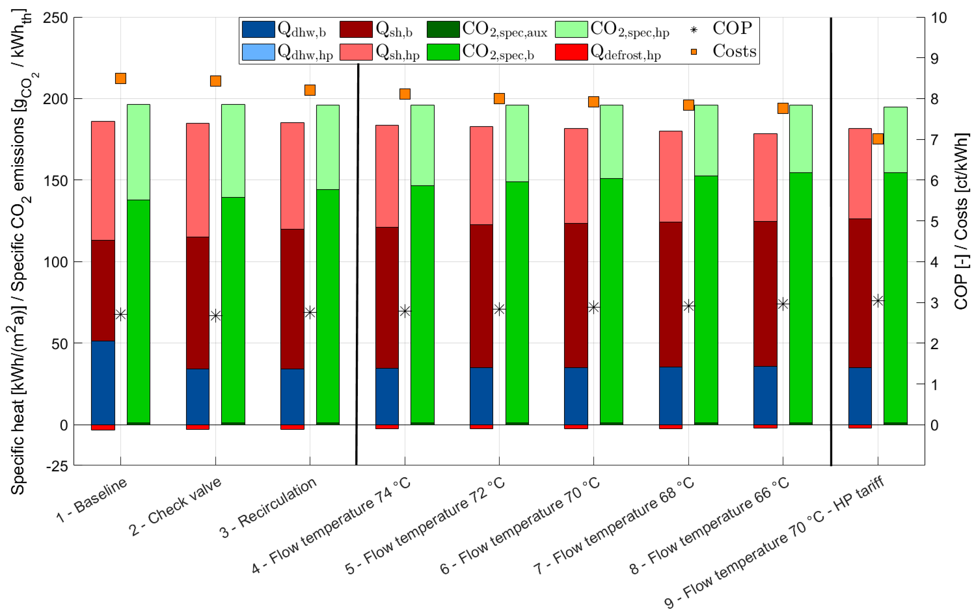
Figure 22.
Comparison of the provided heat and specific CO2 emissions and costs with different improvement measures.
Figure 22.
Comparison of the provided heat and specific CO2 emissions and costs with different improvement measures.
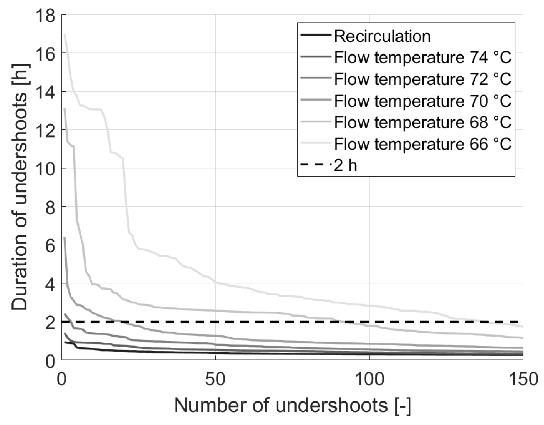
Figure 23.
Zone temperature undershoot time of different applied WCC design set points.
Figure 23.
Zone temperature undershoot time of different applied WCC design set points.
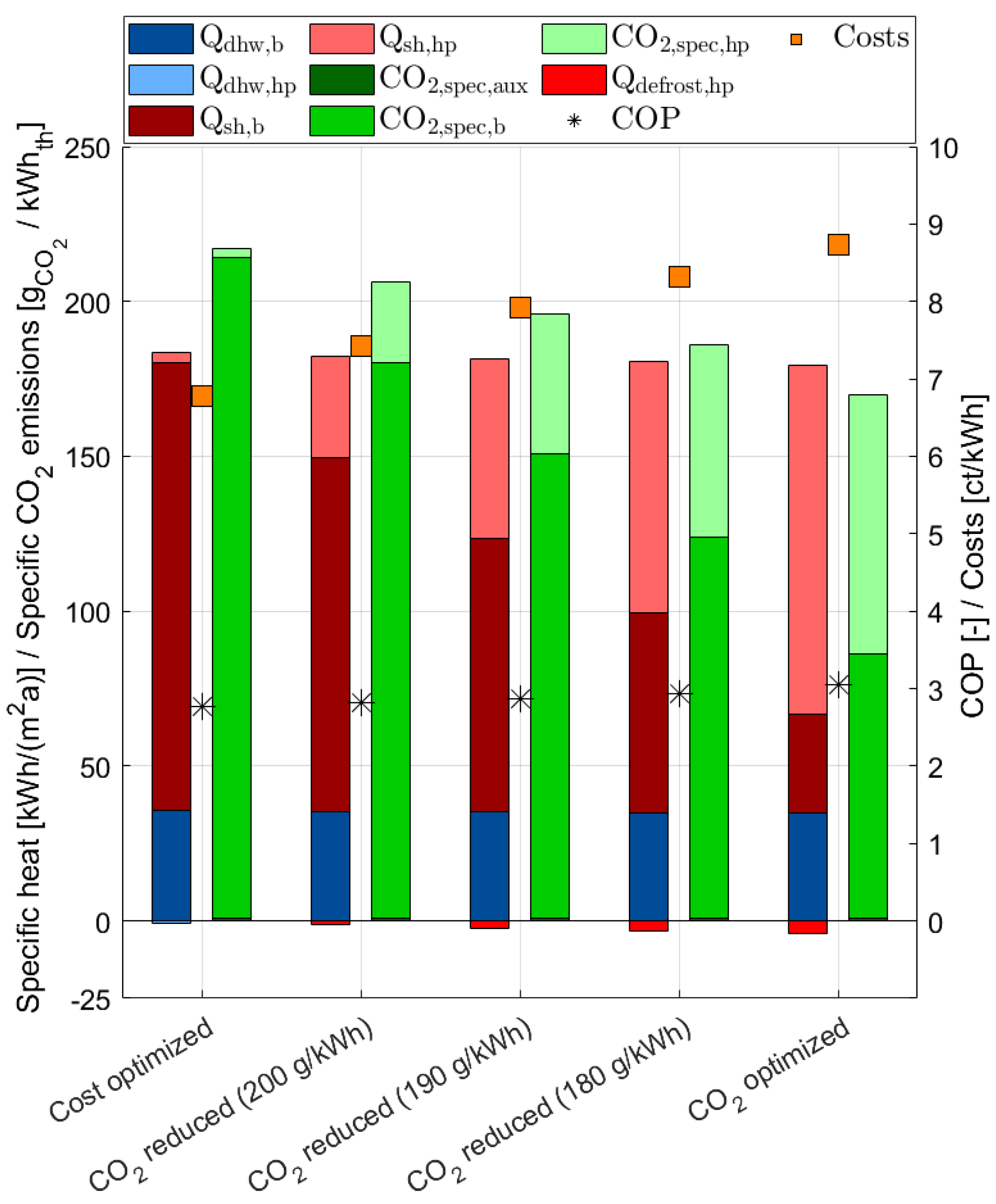
Figure 24.
Comparison of a cost and CO2-optimized strategy with different specific CO2 emission set points of the newly developed algorithm and a household electricity tariff.
Figure 24.
Comparison of a cost and CO2-optimized strategy with different specific CO2 emission set points of the newly developed algorithm and a household electricity tariff.
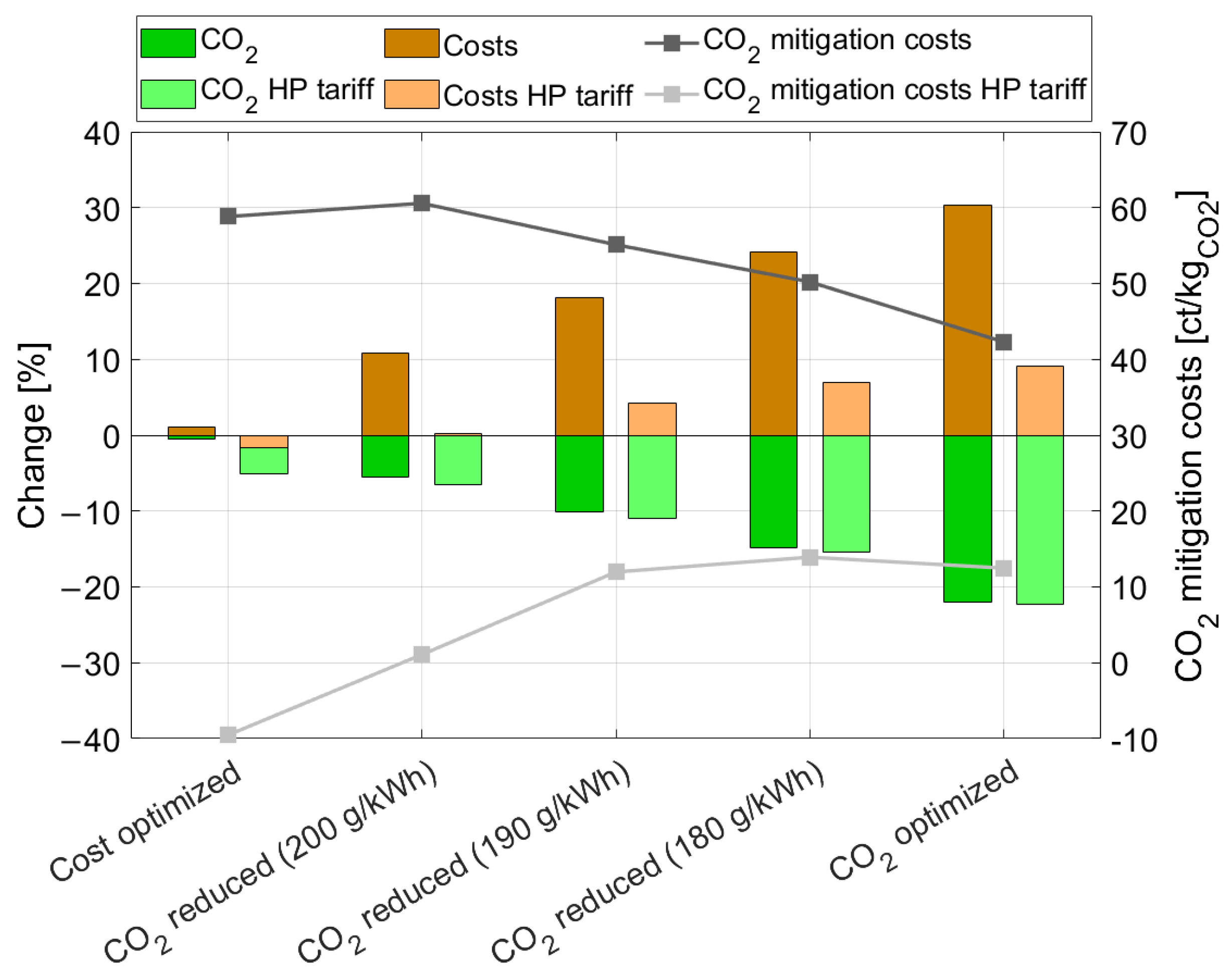
Figure 25.
Changes of CO2 emissions and operation costs with respective CO2 mitigation costs of different operation strategies compared to a boiler system for household and heat pump tariff.
Figure 25.
Changes of CO2 emissions and operation costs with respective CO2 mitigation costs of different operation strategies compared to a boiler system for household and heat pump tariff.
Table 1.
Building data of the field trial.
Table 1.
Building data of the field trial.
| Number of floors | 3 |
| Number of flats (inhabited) | 5 (4) |
| Base area | 151 m2 |
| Window area | 62 m2 |
| Useable building area | 292 m2 |
| U-value exterior wall (W/(m2K)) | 1.40 |
| U-value roof (W/(m2K)) | 1.40 |
| U-value top floor (W/(m2K)) | 1.00 |
| U-value ground floor (W/(m2K)) | 0.56 |
| U-value windows (W/(m2K)) | 1.90 |
| Heat load, transmission | 24.2 kW |
| Heat load, ventilation | 2.7 kW |
| Total heat load | 27.0 kW |
Table 2.
Thermal zones of the building model with respective usage type and heating set point.
Table 2.
Thermal zones of the building model with respective usage type and heating set point.
| Zone Number | Zone Description | Heating Set Point (C) |
|---|
| 1 | Living room | 20 |
| 2 | Kitchen/bath | 20 |
| 3 | Office | 20 |
| 4 | Bedroom | 19 |
| 5 | Cellar/Attic/Stairway | - |
Table 3.
Daily heat load parameter.
Table 3.
Daily heat load parameter.
| | Gas | Electricity |
|---|
| Emission | 222.9 | 404.7 |
| Price | 6.1 | 29.3/22.5 |
Table 4.
Measured and internally calculated provided and used energy with respective deviation.
Table 4.
Measured and internally calculated provided and used energy with respective deviation.
| Property | Measurement (kWh) | Calculation (kWh) | Deviation (%) |
|---|
| Heat | Boiler | 17,978 | 18,181 | 1.3 |
| Heat pump | 17,183 | 17,210 | 0.2 |
| Final energy | Boiler (gas) | 20,415 | 19,979 | −2.1 |
| Boiler (electricity) | 63 | 51 | −18.5 |
| Heat pump | 6441 | 6991 | 8.5 |
| Supply pump P1 | 44 | 45 | 5.7 |
| SH pump | 21 | - | - |
| DHW charge pump | 19 | - | - |
| DHW circulation pump | 21 | - | - |
Table 5.
Provided and used energy with respective deviation in measurement and simulation.
Table 5.
Provided and used energy with respective deviation in measurement and simulation.
| Property | Measurement (kWh) | Simulation (kWh) | Deviation (%) |
|---|
| Heat | Boiler | 17,943 | 17,165 | −4.3 |
| Heat pump | 17,116 | 17,009 | −0.6 |
| Final energy | Boiler (gas) | 20,379 | 19,336 | −5.1 |
| Boiler (electricity) | 62.5 | 48 | −23.5 |
| Heat pump | 6416 | 6268 | −2.3 |
| Supply pump P1 | 44 | 48 | 8.2 |
| SH pump | 21 | 34 | 63.6 |
| DHW charge pump | 19 | 20 | 2.9 |
| DHW circulation pump | 21 | 19 | −7.6 |
Table 6.
Heating set point and mean operative temperature with corresponding undershoot time of the simulated heated zones.
Table 6.
Heating set point and mean operative temperature with corresponding undershoot time of the simulated heated zones.
| Zone Number | Heating Set Point (C) | Mean Operative Temperature (C) | (h) |
|---|
| 1 | 20 | 20.1 | 0 |
| 2 | 20 | 20.4 | 0 |
| 3 | 20 | 20.2 | 0 |
| 4 | 19 | 19.5 | 0 |
Table 7.
Performance indicators of investigated scenarios with different setup changes.
Table 7.
Performance indicators of investigated scenarios with different setup changes.
| Scenario | Nonreturn | Air | Design Flow | | COP | | | Cost | |
|---|
| Valve | Recirculation | Temperature (C) | (%) | (-) | (%) | (g/kWhth) | (ct/kWhth) | (h) |
|---|
| 1 | defect | yes | 76 | 46 | 2.72 | 89.7 | 196.5 | 8.50 | 0 |
| 2 | normal | yes | 76 | 44 | 2.69 | 91.0 | 196.3 | 8.42 | 0 |
| 3 | normal | no | 76 | 41 | 2.76 | 91.3 | 196.1 | 8.21 | 0 |
| Investigation of WCC set point |
| 4 | normal | no | 74 | 40 | 2.80 | 91.4 | 196.1 | 8.11 | 0 |
| 5 | normal | no | 72 | 39 | 2.84 | 91.6 | 196.1 | 8.00 | 7 |
| 6 | normal | no | 70 | 38 | 2.88 | 91.7 | 196.0 | 7.92 | 52 |
| 7 | normal | no | 68 | 37 | 2.92 | 91.8 | 196.0 | 7.85 | 296 |
| 8 | normal | no | 66 | 36 | 2.96 | 91.9 | 196.0 | 7.76 | 673 |
| Heat pump electricity tariff |
| 9 | normal | no | 70 | 36 | 3.05 | 91.7 | 194.9 | 7.01 | 37 |
Table 8.
Performance indicators of different operation strategies with household and heat pump electricity tariff.
Table 8.
Performance indicators of different operation strategies with household and heat pump electricity tariff.
| Scenario | (%) | COP (-) | (%) | (g/kWh) | Cost (ct/kWh) |
|---|
| Household electricity tariff |
| Boiler | - | - | 93.2 | 218.1 | 6.71 |
| Cost opt. | 2 | 2.72 | 93.2 | 216.9 | 6.78 |
| 200 g/kWh | 21 | 2.82 | 92.5 | 206.2 | 7.43 |
| 190 g/kWh | 38 | 2.88 | 91.7 | 196.0 | 7.92 |
| 180 g/kWh | 53 | 2.94 | 90.6 | 185.9 | 8.33 |
| CO2 opt. | 74 | 3.05 | 87.7 | 170.0 | 8.74 |
| Heat pump electricity tariff |
| Cost opt. | 11 | 4.13 | 92.8 | 207.7 | 6.62 |
| 200 g/kWh | 18 | 3.40 | 92.6 | 204.5 | 6.74 |
| 190 g/kWh | 36 | 3.05 | 91.7 | 194.9 | 7.01 |
| 180 g/kWh | 52 | 3.00 | 90.6 | 185.0 | 7.20 |
| CO2 opt. | 74 | 3.05 | 87.7 | 170.0 | 7.34 |


