1. Introduction
Drilled lithology is among the most significant real-time factors influencing the decision in drilling operations, useful for the prediction of drilling fluid lost circulation, parameter optimization in drilling, reducing shale problem, and maintaining wellbore stability. Lithology identification can be divided into direct and indirect measurements. Logging while drilling (LWD) tools and surface measurements are directly measured to optimize drilling operations. Surface measurements include analysis of cores and drilling cuttings, which are time-consuming and expensive. Some drilling parameters such as the rate of penetration (ROP), cuttings analysis, hook load, weight on bit (WOB), and surface torque are used in intelligence models to estimate lithology indirectly.
LWD tools, placed 20–30 m above the drilling bit in the drill string, provide crucial information about reservoir characteristics and downhole conditions. The most widely used LWD tools are density, caliper, resistivity, and neutron log. They are attributed to lithology types drilled in the wellbore. However, due to their place in the drill string, LWD tools provide information about previously drilled lithology, which might not be considered real-time lithology.
Surface measurement involves cutting analysis and drilling hydraulics. Similar to LWD, cutting analysis provides slightly delayed information about real-time lithology. Drilling hydraulics such as WOB, surface torque, and ROP information can be attributed to drilled lithology in real-time. Machine learning techniques are useful in constructing predictive models for lithology prediction from drilling data. Like the cutting analysis technique, the image process of core samples is used for lithology classification using core CT images. The conventional CT image interpretation, such as direct visual inspections by geologists, is time-consuming and a subjective interpretation that might lead to wrong classifications. In addition, the extraction of detailed core data requires high capital investment. Therefore, machine learning algorithms are employed to identify lithology types quickly. The authors of [
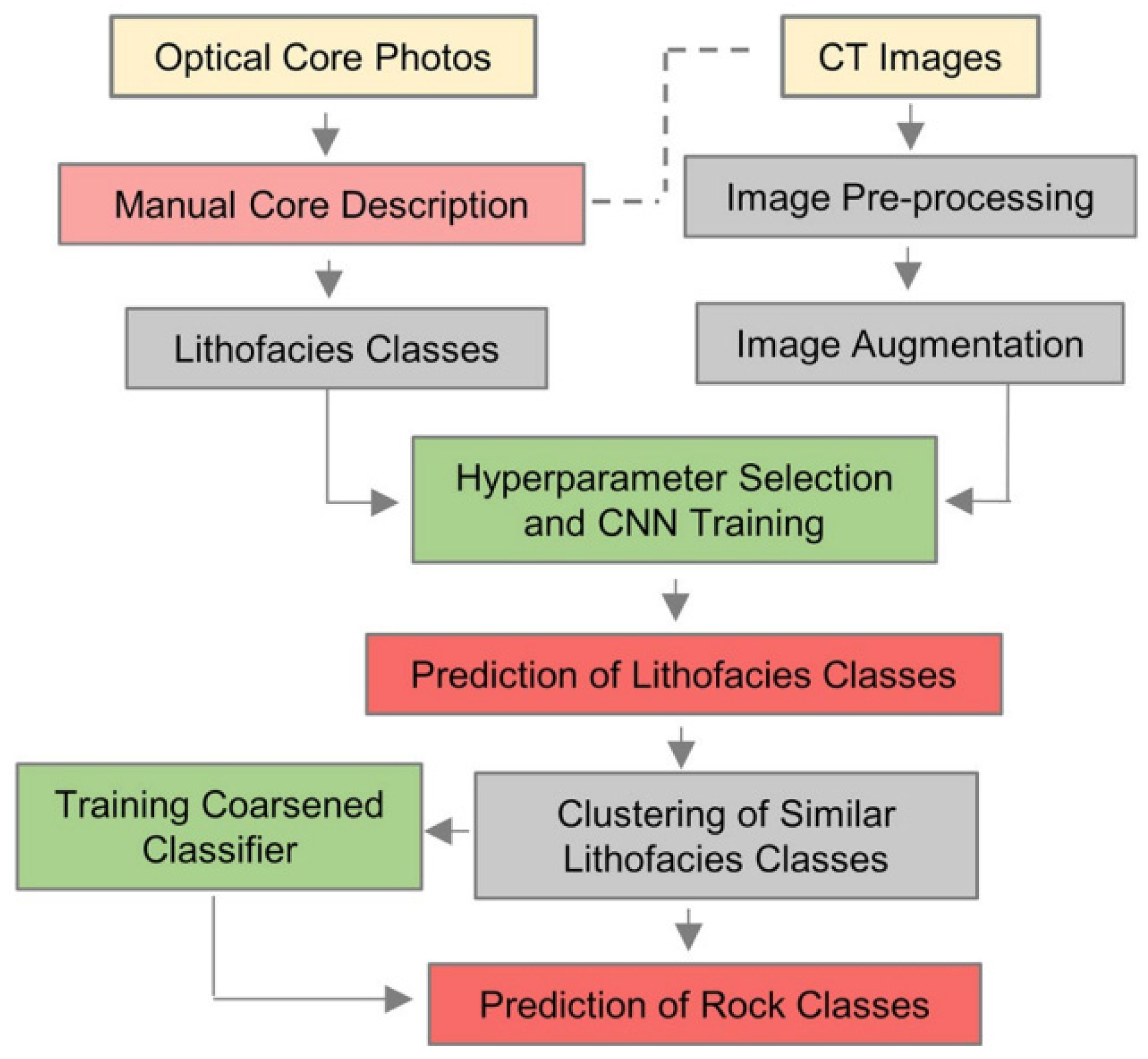
1] used convolutional neural networks (CNN) to classify the lithology of whole core CT scans. The proposed workflow for lithofacies classification is shown In
Figure 1. Reprocessing of 2D images is the first step of the workflow. The next step is labeling images depending on identical geological descriptions. The CNN model uses the labeled images for training. As a standard application, the data set is divided into 80 and 20% for training and testing, respectively. The trained model is then validated against lithofacies, and the model classifies the lithofacies based on images. To increase the performance of CNN, image augmentation is performed. As a similar working principle, Ref. [
1] classified the lithology of core CT scan images using a deep learning approach. In this case, they used 3D information as inputs in CNN. The performance of the trained classifier was evaluated with an untrained set of images to estimate formation. They used sub-cubes instead of full three-dimensional images resulting in a higher amount of training images; therefore, a smaller interval of the well is needed for model training. The prediction results show that the classifier generalizes well, achieving an overall accuracy of 0.97. The calibrated model showed good performance pixelwise and in terms of heterogeneity of high resolution.
The interaction between drilling bits and formation is different for lithology types. The authors of [
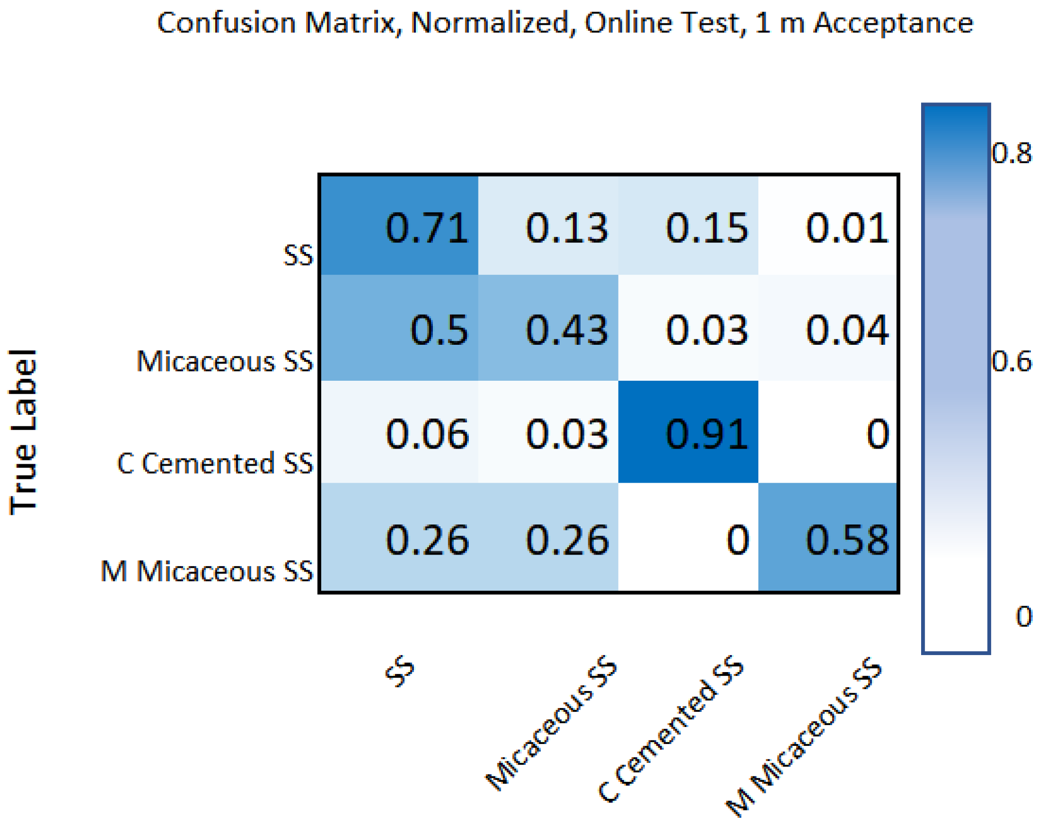
2] used deep learning to classify drilled lithology in real-time. They used surface-measured drilling parameters and LWD logs as inputs to classify lithology with multilayer perceptron (MLP) models. They estimated four different lithologies: sandstone, calcite cemented sandstones, muddy micaceous sandstone, and micaceous sandstones. Since LWD measurements are not available in real-time, surface measurements were used as an intermediate step to estimate virtual logs. The input parameters to estimate the virtual logs were WOB, RPM, torque, hook load, and ROP. Poor results were obtained for the caliper and resistivity log. The MLP model included five hidden layers, with 10 nodes for each layer. The performance of the proposed model on the calcite cemented sandstone class was high because of its hardness, which made it easier to distinguish. The other three lithologies showed similar characteristics, confusing the model (
Figure 2).
Statistical and intelligence methods are applied in the well log to estimate lithology during drilling. Ref. [
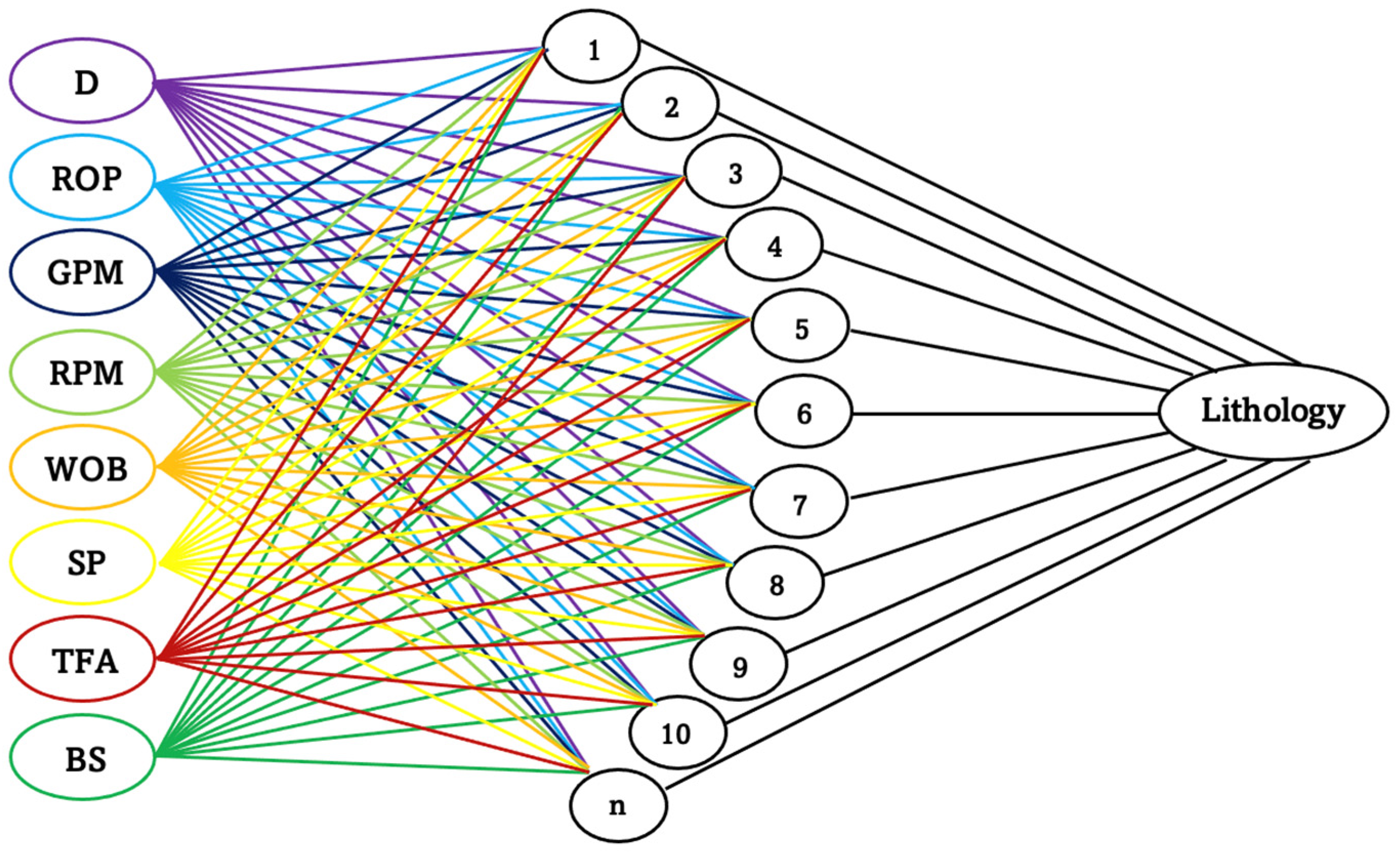
3] used an artificial neural network (ANN) to identify 10 different lithologies such as gypsum, siltstone, shale, claystone, salt, and anhydrite, marl, limestone, sandstone, and dolomite (
Figure 3). They used drilling data as inputs for ANN to estimate lithology (
Table 1). The model trained 2757 samples of a drilled well. The average absolute error was 4.01%.
In mature oil and gas fields, drilling data of nearby wells can be used as supplementary to new drilling data in real time to estimate real-time drilling lithology. Ref. [
4] used drilling parameters such as WOB, pump pressure, and ROP in an ANN to estimate real lithology. They used 70% of the dataset for training, and the remaining data were used for testing and verification. The model verification was tested with an R-squared value, which was 0.8742.
1.1. Machine Learning Applications in Fracturing Operations
Fracturing technology has been a common practice since the 1950s to improve production in tight formations. Lithology is one of the critical parameters determining fracture extent in the pay zone and the fracture geometry. Fracture growth through different layers shows a great difference based on the formation’s characteristic properties. Therefore, it is essential to identify facies and optimize treatment parameters accordingly. A considerable amount of data has been generated from the fracturing operations conducted. Machine learning approaches are good at analyzing, evaluating, and categorizing the data with their strong learning and prediction capability. As the literature is reviewed, it was found that most machine learning approaches are about parameter optimization during treatment. The authors of [
5] studied optimization of hydraulic fracturing design from several thousand of multistage frac jobs with machine learning. The study focused on the gathering, cleaning, and processing of the data. A similar fracturing optimization workflow was proposed by [
6]. They used three supervised algorithms which are K-nearest neighbor (KNN), radial basis function (RBF), and multilayer perceptron (MLP) to associate fracture properties and productivity of shales (
Figure 4). RBF and MLP showed higher net present values (NPVs) comparing to KNN in a proxy model.
Logistic regression has been incorporated with RBF to improve the classification performance of RBF neural network in the classification of hydraulic fracturing [
7]. They used binary classification to generalize multi-classification problems. The study reported very good generalization properties in highly overlapping simulation data. Proppant classification is the other part of hydraulic fracturing where machine learning algorithms are employed. Ref. [
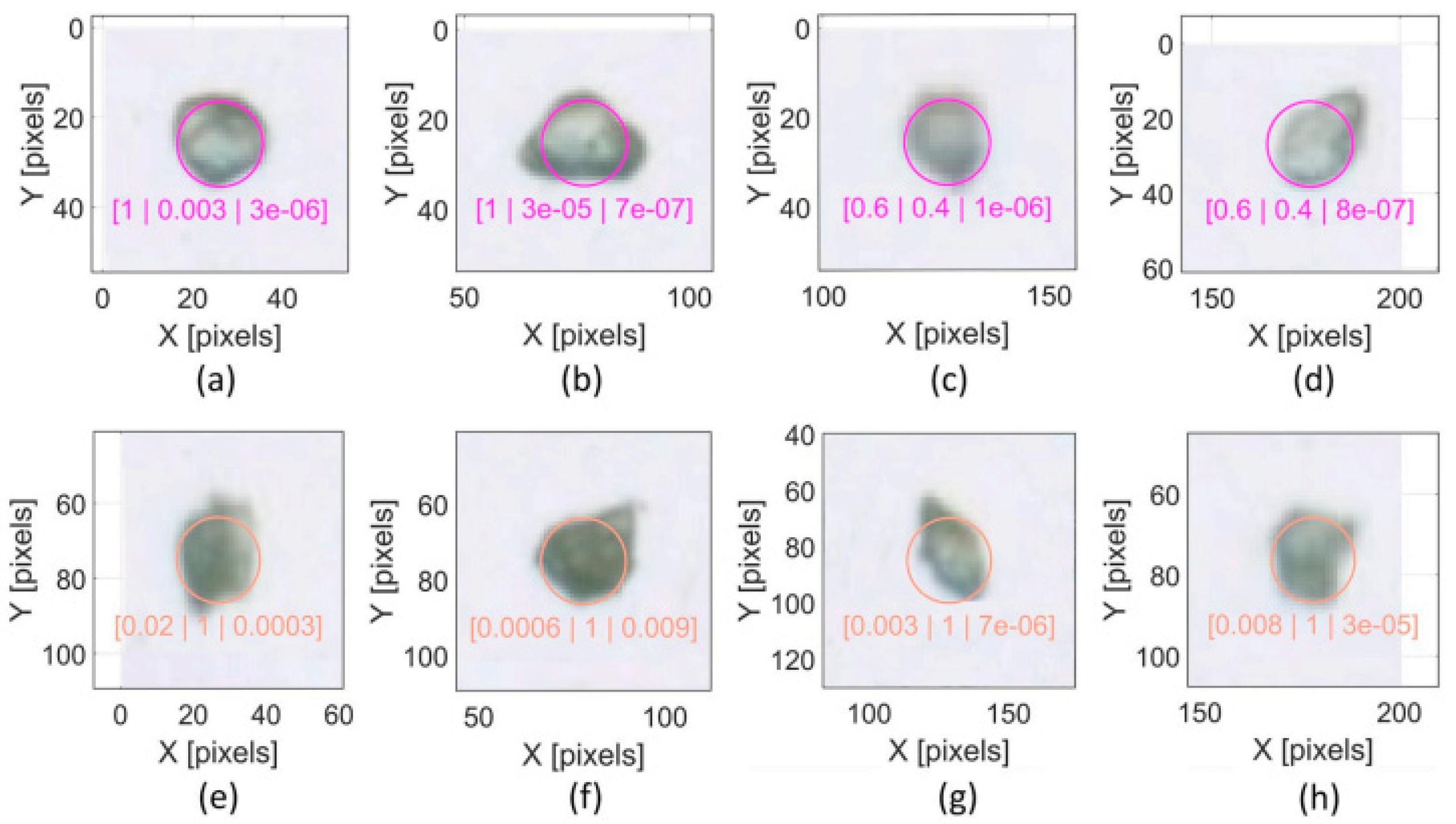
8] designed an efficient proppant detection and classification program for subsurface formations using machine learning. They applied the supervised ANN-based classification workflow on the proppant distribution from the Permian basin. Validation of ANN was carried out with K-fold. The classification algorithm detected calcite and proppant particles (
Figure 5).
Nonlinearity and the multi-dimensional characteristics of log data increase the challenges for accurate estimation of lithology. That is why the traditional statistical methods such as histogram plotting provide poor results. Researchers have applied unsupervised learning methods in the last decades. To illustrate, Ref. [
9] combined principal component analysis (PCA) and cross plot to obtain information about lithology identification. Ref. [
10] used a modified K-means clustering technique to classify lithology. Ref. [
11] estimated lithology type using PCA and wavelet analysis. The unsupervised learning approach classifies formations depending on the data properties; however, the accuracy of the models is generally lower than supervised learning [
12]. Ref. [
13] compared results obtained from unsupervised learning, supervised learning and neural network models for lithology classification. The study showed that supervised methods provide better classification results compared to other methods (
Table 2).
Unsupervised classification algorithms classify the data into a certain number of sets to best represent the provided data. The data are with no pre-interpretation for any given group. Biasing the training data might provide interpreter control of the output. Ref. [
14] compared machine learning techniques such as k-means clustering, principal component analysis (PCA), unsupervised Bayesian classification, and waveform classification to classify facies in the Delaware Basin. They also used self-organizing maps, independent component analysis (ICA), and generative topographic mapping. PCA is used to reduce the dimension of the data and assumes a Gaussian distribution. The covariance matrix is used to reduce the number of attributes.
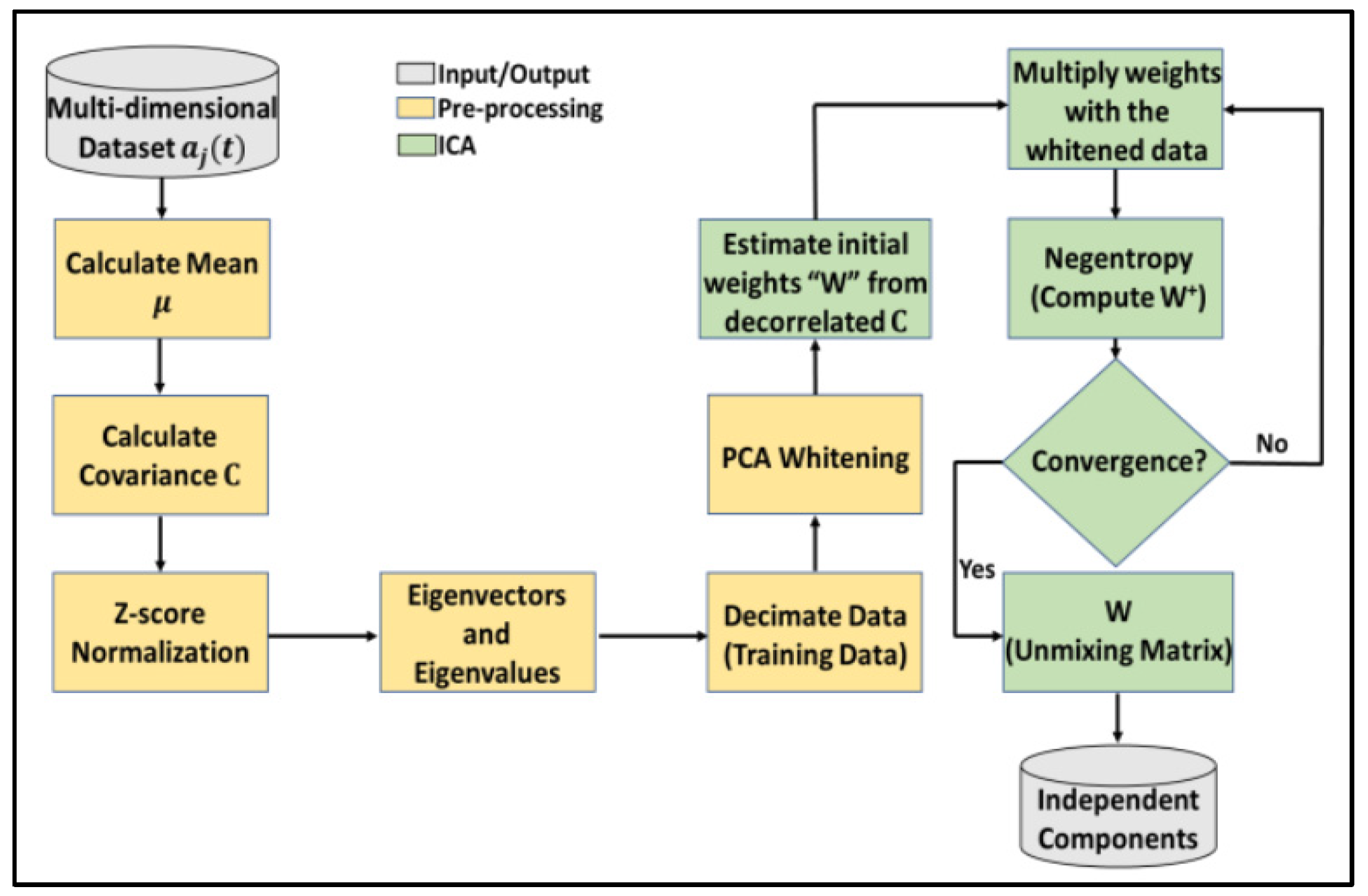
ICA divides multivariate data into independent parts. K-means clustering is one of the easiest classification algorithms used to interpret seismic attributes. The clustering algorithm begins with assigning at random k centroids, serving as centers of the groups to form. The distance between each datum and centroid is calculated. Thus, the points are classified according to this calculation process. Self-organizing maps create a seismic facies map from various seismic interpretations with an unsupervised approach. The supervised learning answers the questions defined; however, the unsupervised technique can classify a group of undefined and distinct class, but it does not provide indications of what it means geologically. The study showed that ICA provides more details than PCA. Ref. [
15] used ICA to classify seismic facies with the proposed workflow shown in
Figure 6. The study found that ICA is a robust method for reducing dimensionality and noise in multiple seismic attributes.
1.2. Machine Learning Applications in Fracturing Operations
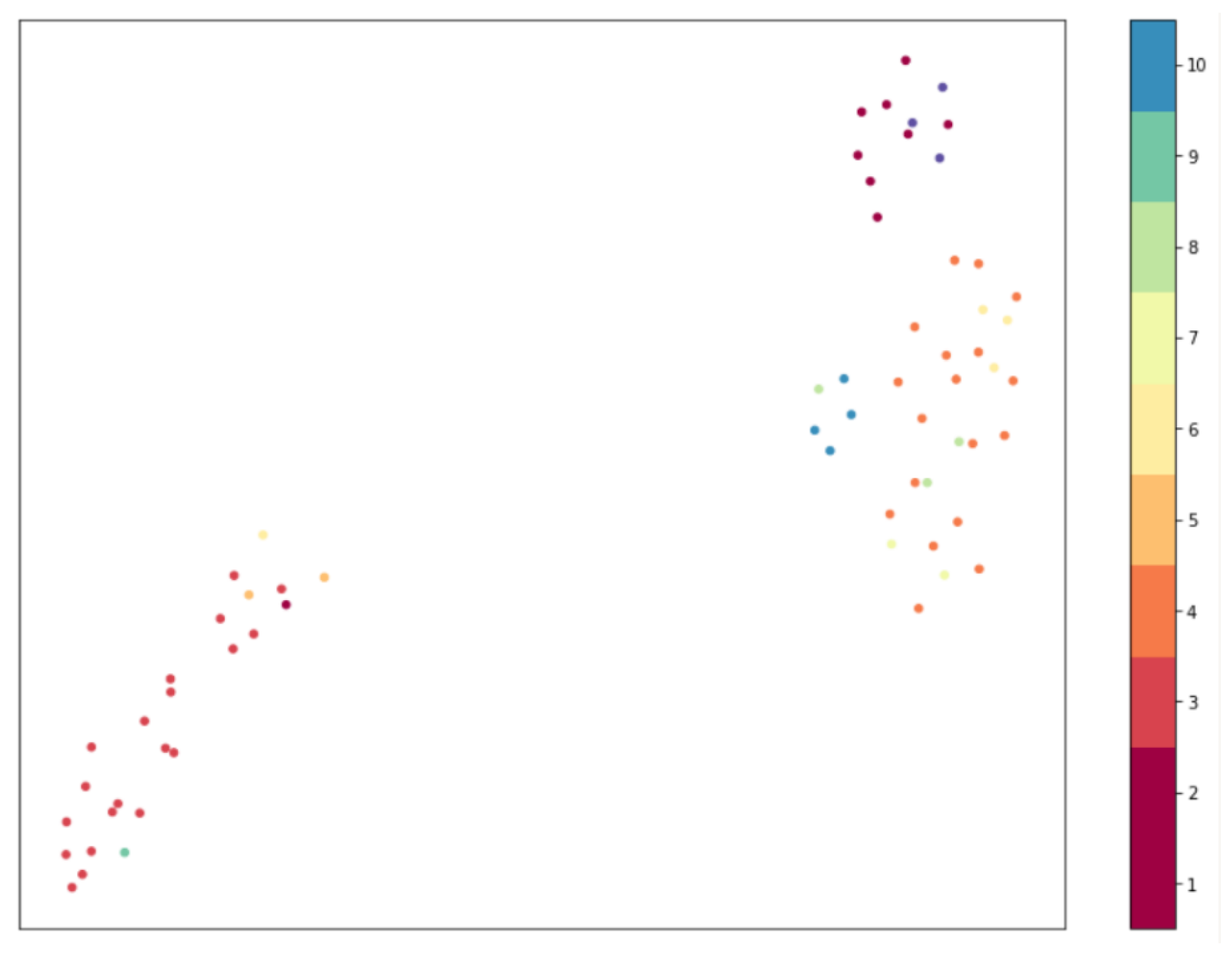
An unsupervised map (UMAP) is a new technique providing low runtime while maintaining the data structure [
16]. In its simplest form, UMAP builds a high-dimensional plot of data and then optimizes a low-dimensional graph with a similar structure. UMAP builds a complex fuzzy representing a weighted graph. Edge weights indicate two connected points. A radius that extends outward from each point is used to test the connectedness of the points. A small radius means small isolated clusters, and a too large radius causes the connecting of all points together. Therefore, choosing an optimum radius is critical in this process. UMAP uses the following methodology: a local radius is first selected considering the distance from each data to its neighbor. Then, the likelihood of points’ connection decreases as the radius grows. The two commonly used parameters to balance between local and global structures are min_dist and n_neighbors (
Figure 7). This study uses UMAP as a remarkably simple tool to classify facies with the help of high dimensionality and good scaling of the dataset.
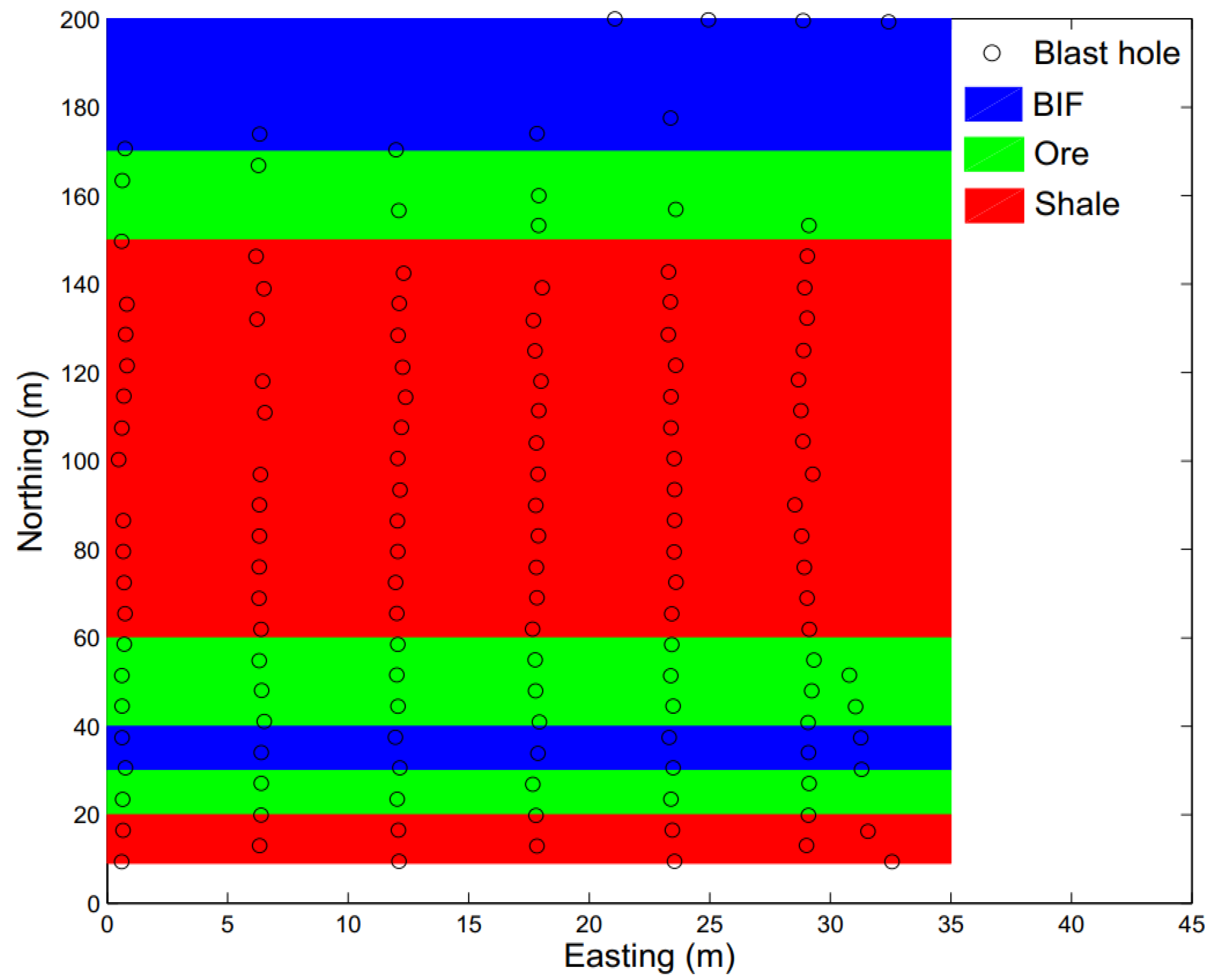
Drilling data include a broad of indication about lithology type. The supervised approach uses the data relating to estimating formation properties. However, unsupervised methods group the parameters based on certain properties, even if there is no relation between datasets. Ref. [
17] proposed an adaptive unsupervised method to estimate formations by minimizing the entropy gradient of the characterizing measurement while drilling. They conducted experiments on the mining data, involving the three major rock types which are BIF, ore, and shale. As shown in
Figure 8, the red section illustrates shale, the blue represents BIF, the strongest rock, and the green shows ore with intermediate strength.
The lithology estimation from drilling surface data was studied by [
18], as one of the main aims of scientific drilling in Nankai through the Seismogenic Zone Experiment. They first estimated drilling torque along the profile from the bottom of the well to the surface. Then, the lithology was estimated from the surface drilling data with neural network algorithms (
Figure 9). The classification process was carried out on the sand, silt clay, and volcanic ash by learning with two layers and an L1 regularization coefficient of 10. A high goodness score (95%) was reported with the complex network.
2. Materials and Methods
The geological process of rock formation has significant impact on the flow and transport in porous media. Digital rock is used as an analogy to estimate the relation between features of the flow system such as aperture, porosity, and permeability. This study includes facies classification derived by grouping facies based on corresponding features such as porosity and permeability. The data samples were retrieved from digital rock samples created by [
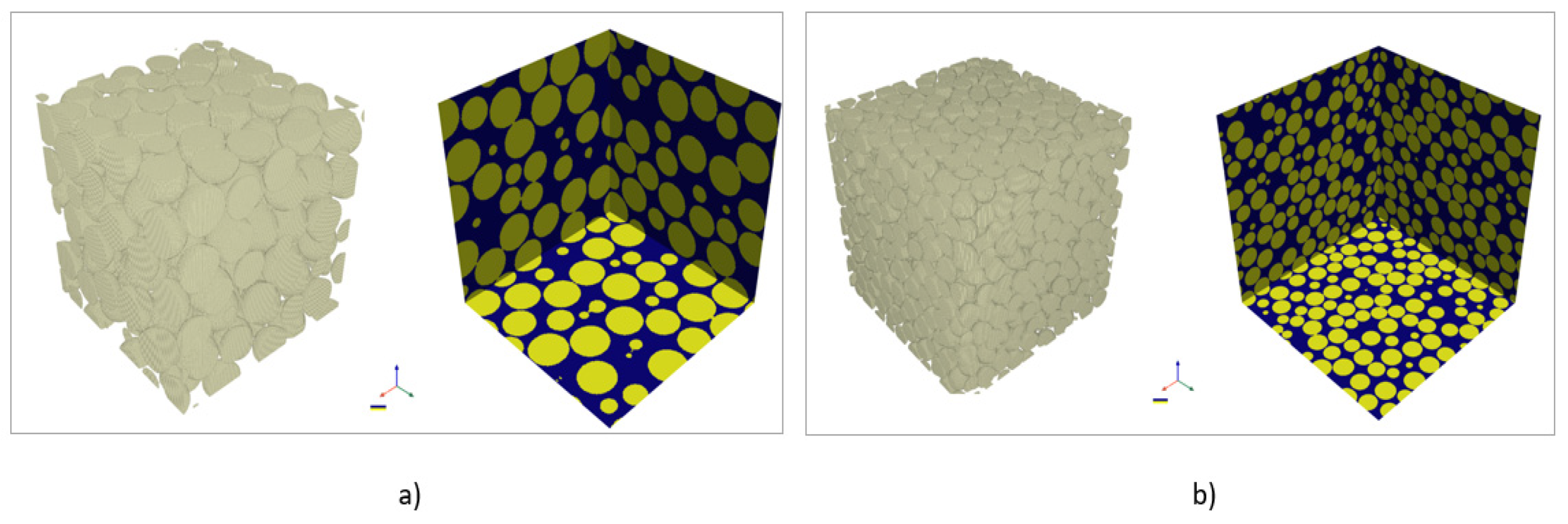
19]. Digital rock images represent the complexity of rock systems. The source of digital rock is either an image of actual rock and soil or based on geostatistical and stochastic models. A regular grid or meshing operation is commonly applied to use digital images in numerical simulations. A 3D binary geometry in a standardized format was used to show the variety of geological features representing different depositional systems and diagenetically processes. The dataset was stored in 66 folders involving different synthetic facies classes in “. mat” files format. The data were then converted into .csv format before using in the simulations. It is important to note that most images have “256” pixels. Therefore, images with “256” resolution were kept, while images with “480” were removed from the data sample.
Figure 10 shows a digital rock with 256 and 480 samples. The porosity of the image with 256 samples was 0.36, and it was 0.362 for the image with 480 samples.
Figure 11 represents a digital rock with 44 and 22mm fracture apertures.
In this study, we have used supervised and unsupervised machine learning algorithms to classify facies. The main distinction between the two approaches is the use of labeled data. Supervised learning uses labeled and output data, while unsupervised learning does not. The workflow for the unsupervised model is shown in
Figure 12. The data was handled as numerical and image variables for the preparation and cleaning process. Various learning algorithms were employed for training operations, such as anomaly detection, double median absolute deviation, local outliers, and baseline image models.
Median absolute deviation (MAD) algorithm is a frequently used algorithm for anomaly clustering. The median of all the time series at one time shows normal behavior for all the time series at that time. The anomalous are detected from large deviations from each individual time series and median. The main challenge with anomaly detection is reducing the number of false positives and noisy alerts. MAD algorithm overcomes this issue by monitoring the outputs at a specified window. As the individual series output reaches a specified percentage of anomalous points, the series is classified as anomalous.
Image baseline model can flag anomalous images that are not encountered in a baseline of images used for training. The baseline model shows which feature is important for prediction and which is not. The first step is score calculations, and then feature engineering of the dataset is applied. The addition of a new feature to the model is monitored with the score of baseline machine learning. A better score means the success of the new feature for predictions.
An isolation forest works like random forest models. It recognizes anomalies by detecting points called “few and different”. The algorithm trains the data with an ensemble of binary decision trees and generates isolation trees based on randomly selected features.
The local outlier factor (LOF) algorithm is an unsupervised outlier detection method computing the local density deviation of a given data point with respect to its neighbors. The outlier samples are detected based on their lower density than that of neighbors.
The supervised algorithms used in this study were eXtreme Gradient Boosted Trees, Keras Slim Residual Neural Network, Elastic-Net Regressor, and Keras Deep Residual Neural Network. The supervised model workflow is shown in
Figure 13.
The gradient boosting (GB) technique is used in both regression and classification tasks. XGBoost a type of GB, usually provides higher accuracy than a single decision tree. XGBoost uses a second-order Taylor approximation in the loss function.
A residual neural network is a neural network consisting of residual building blocks. RNN has gained popularity with its impressive image classification performance. A skip connection added to weighted layers allows information to pass more freely and the gradient to be more realistic. The residual unit uses convolution, batch normalization, and rectified linear unit to learn the residual mapping function [
20]. The deep residual neural network has a similar working principle but provides many network layers, which is favorable for capturing the complex statistics of digital images.
The elastic net regression model is a form of regularized optimization for linear regression. It is used to learn compact projection matrices and to enlarge the margins of different classes, which is essential for classification tasks [
21].
3. Results and Discussions
The comparative performance of unsupervised models for best anomaly detection is shown in
Table 3. Double median absolute deviation showed the best accuracy compared to other unsupervised models. As
Table 4 shows, among the supervised learning models, the eXtreme gradient boosted trees regressor showed better validation than other learning techniques. It was also found that the supervised validation (0.85) was better than that of unsupervised validation, which was 0.80. The image classification of supervised learning methods is more accurate than unsupervised ones.
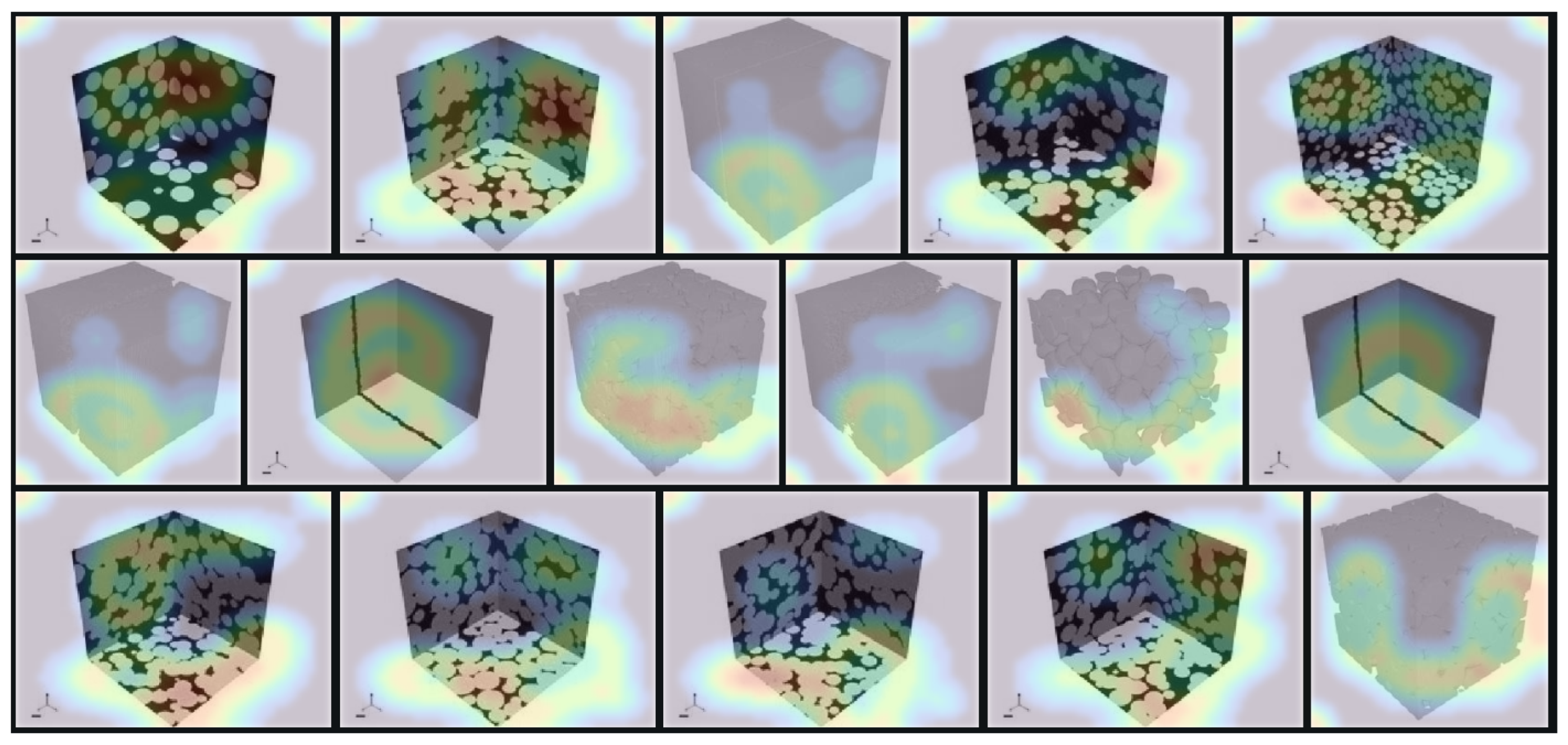
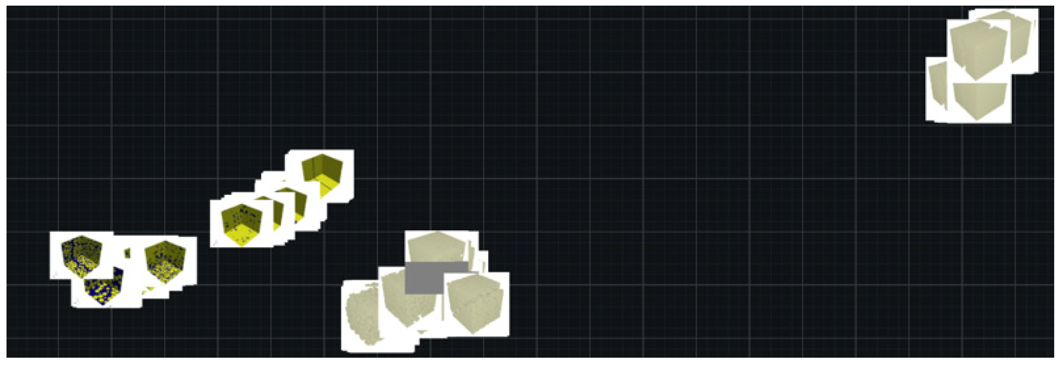
Activation maps are a simple technique for obtaining the discriminative image regions to identify a specific class in the image. They enable us to identify which regions in the image were relevant to the class. In this study, we tried to capture discriminative image regions with unsupervised and supervised learning approaches (as illustrated in
Figure 14). The latter technique (as illustrated in
Figure 15 and
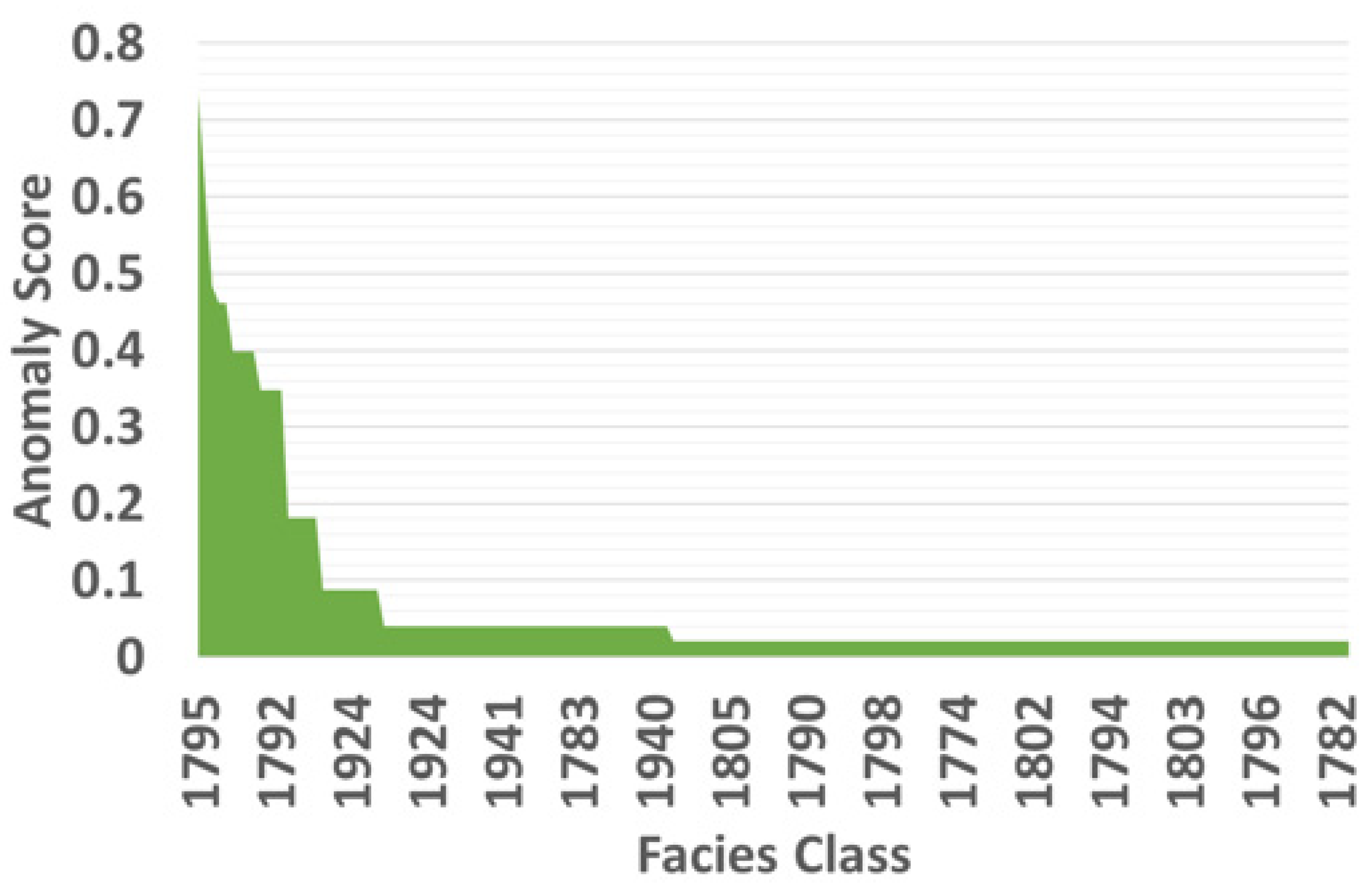
Figure 16) identified the relevant regions better than the former. Anomaly score decreased with the increase in the number of facies in the simulations. Therefore, image classification with supervised learning (as illustrated in
Figure 17) outperforms that obtained with unsupervised learning (as illustrated in
Figure 18).
