Vom Berg and Hahn–Eyring Drilling Fluid Rheological Models

Abstract

This article presents rheological models of fluids used in the drilling practice. It discusses the principles of determining drilling fluid rheological parameters based on data acquired from measurements by means of viscometers used in the drilling practice. The authors propose the application of the three-parameter Vom Berg and Hahn–Eyring models not used in the drilling industry so far. Necessary relationships have been developed for these models, which enable the determination of rheological parameters. In order to account for the influence of different flow conditions on the value of drilling fluid rheological parameters, the approach proposing the determination of rheological parameters of a given three-parameter model separately for low shear rates and high shear rates has been suggested. A practical application of the methodology proposed in this paper for determining the rheological parameters of the three-parameter Vom Berg and Hahn–Eyring models is presented using real drilling fluids as an example. Using the author’s methodology for determining the optimum rheological model, called Rheosolution, described earlier in the paper “Selection of Suitable Rheological Model for Drilling Fluid Using Applied Numerical Methods”, published in Energies 2020, 13, 3192, and laboratory tests performed for this work (for cement slurries according to API standards), a strong correlation of the Vom Berg model and, in particular, the Hahn–Eyring model for such drilling fluids was demonstrated.

1. Introduction

Drilling fluids such as drilling muds, drill-in fluids, fracturing fluids, spacers, wash fluids, and cement slurries are commonly used in the oil-drilling industry. The recognition of the phenomena occurring in the borehole during the flow of technological fluids makes it possible to avoid or reduce drilling failures and complications, such as the loss of circulation in the borehole, eruptions of reservoir fluids, tightening, caving of the borehole wall, and the sticking of drilling tools, drill pipes, or casings installed in the borehole. The flow of drilling fluids is limited by pressure losses in the circulation system. By correctly identifying and adjusting the rheological model, it is possible to reduce the total pressure loss throughout the entire system, thus reducing the cost of the drilling process [1,2]. Studies conducted at the Drilling Oil and Gas Faculty Department of Drilling and Geoengineering for cement slurries and drilling muds confirm that three-parameter models most accurately describe the rheological properties of actual drilling fluids. The American Petroleum Institute API RP 13D recommends using one of the three models: Bingham, Ostwald–de Waele (power law), or Herschel–Bulkley (yield power law) [3,4,5,6]. A proper selection of the physical parameters, rheological properties, and technologies of drilling fluid application has a considerable impact on the costs of making boreholes and the safety of drilling works [1,2,7,8].

A primary challenge that needs to be resolved in order to understand the phenomena occurring during the circulation flow of drilling fluids is to determine the effective relationship between the flow rate of the fluid that is pumped and the flow resistances that occur during pumping. Depending on the adopted rheological model applied for the description of physical phenomena occurring during drilling fluid flow, different calculation formulae are used and different results are obtained [8]. A rheological model is only an approximated description of the properties of real drilling fluid, whereas different calculation results stem from the precision of determining the rheological parameters of the model concerned. Therefore, it seems appropriate to apply such a rheological model that will describe the rheological properties of real drilling fluid in the most precise way. The three-parameter Vom Berg and Hahn–Eyring models were used in the research laboratory tests. These rheological models were used to describe the rheological parameters of other fluids [9] and have been described in detail [9,10]. In the research study, a high correlation between the proposed rheological models and the drilling cement was noted. Laboratory tests carried out by other scientists also support this [11,12]. As a result and according to API standards [3,7,8,13,14,15], samples of fresh cement slurries were prepared. The water–cement ratio of the prepared cement slurries ranged between 0.38 and 0.56 depending on the depth of application. Viscosity measurements were performed by the use of a Chan model 3500 (Section 5) and Fann model 35A/SR-12 (Section 6) viscometer in accordance with the API specification [15].

2. Drilling Fluid Rheological Models

Technological fluids used in engineering practice can be described by different rheological models.

Real fields subject to external forces are deformed, whereby such deformation results from a change in the mutual location of particular field elements. Rheology is the science concerning the deformation and flow of matter [16]. It relates to the mechanics of real fields, subject to deformation under the influence of external forces. Deformations can be divided into elastic, plastic, and flow. Elastic deformation occurs when it is spontaneously reversible, i.e., it disappears when force stops operating. Plastic deformation is irreversible, i.e., it does not disappear when force stops operating. Flow is also an irreversible deformation, which increases continuously with time under the influence of force operation.

Fluids used for the needs of the drilling sector, including drilling muds, cement slurries, and fracturing fluids, can be divided into [8]:

• Generalized Newtonian fluids;
• Non-Newtonian fluids.

Generalized Newtonian fluids are fluids for which the dependence between stress and the shear rate has the form of τ = μ(−dv/dr)ⁿ. A special case of this kind of fluid is classical Newtonian fluid, for which a flow curve is a straight line passing through the origin of the coordinates.

Non-Newtonian fluids are fluids for which a flow curve is straight or curvilinear and does not pass through the origin of the coordinates. They include Bingham plastic fluids and fluids showing both Bingham plastic and pseudoplastic properties.

The majority of fluids used in the drilling industry are Newtonian, Bingham plastic, and pseudoplastic fluids [5,6,7,8]. The application of chemical agents enabling the modification of the physical properties and rheological parameters of drilling muds causes muds to possibly demonstrate both the features of Bingham plastic fluids and pseudoplastic fluids.

The API RP 13D standard, with recommendations concerning the rheological studies and hydraulic calculations of drilling fluids, recommends applying one of the following three models: Bingham, Ostwald–de Waele (power law), or Herschel–Bulkley (yield power law) [1].

• The Bingham model:

$$\tau ={\tau }_y+\eta \cdot \left(-\frac{dv}{dr}\right)$$

(1)

• The Ostwald–de Waele model (power law):

$$\tau =k\cdot (-\frac{dv}{dr}{)}^n$$

(2)

• The Herschell–Bulkley model (yield power law):

$$\tau ={\tau }_y+k\cdot (-\frac{dv}{dr}{)}^n$$

(3)

The studies on drilling fluids (drilling muds, drill-in fluids, spacers and washes, cement slurries, fracturing fluids) performed at the Faculty of Drilling Oil and Gas, AGH University of Science and Technology in Kraków, prove that in the vast majority of cases, the Heschel–Bulkley model can be assumed as the one most precise for describing the rheological properties of real drilling fluids [5]. This model is a three-parameter model $\left({\tau }_y,k,n\right)$, contrary to the two-parameter Bingham $\left({\tau }_y,\eta \right)$ and power law $\left(k,n\right)$ models.

For drilling fluids, other three-parameter rheological models should also be considered [9,17,18,19].

One of the models able to be applied is the Vom Berg model, in the following form [17,19]:

$$\tau ={\tau }_y+D\cdot sin h^{-1}\left(\frac{-\frac{dv}{dr}}{C}\right)$$

(4)

Alternatively, the application of the Hahn–Eyring model is proposed [3]:

$$\tau =E\left(-\frac{dv}{dr}\right)+D\cdot sin h^{-1}\left(\frac{-\frac{dv}{dr}}{C}\right)$$

(5)

3. Mathematical Foundations for Determining Rheological Parameters by Means of the Vom Berg and Hahn–Eyring Models

The rheological properties of drilling fluids are measured by means of rotational viscometers of the following types: Fann, Chan, Brookfield, Haake, and Ofite [20,21,22,23,24]. A fluid test consists of determining shear stress relationships $\left(\tau \right)$ as a function of shear rates $\left(\dot{\gamma }=\left(-\frac{dv}{dr}\right)\right)$.

Drilling fluid rheological parameters are specified on the basis of standard [8], as well as relationships that are developed and not accounted for in standards [9,25]. Standards [8] and [26] recommend the use of Fann viscometers (drilling muds, drill-in fluids, fracturing fluids) and Chan viscometers (spacers and washes, cement slurries). In those viscometers, fluid fills the space between two cylinders: external (rotor) and internal (bob). Tests are carried out to record the dependence of a torsion angle of an internal cylinder on the rotational speed of an external cylinder. The shear stresses being determined are proportionate to a torsion angle of the internal cylinder (bob) towards the external cylinder (rotor), rotating with constant rotational speed [8,20].

Shear stress depends on a torsion spring angle ($\varnothing$), spring constant (K_s), and stresses on one degree of spring torsion (τ₁). They are determined from the following formula:

$${\tau }_i={\varnothing }_i{K}_s{\tau }_1$$

(6)

Laboratory testing of the cement slurries and drilling muds described in this paper was carried out using Fann and Chan viscometers. The shear stress per degree of torsion angle of the installed F1 spring was 0.511 (Pa/gradian) [20].

The shear rate of fluid $\left({\dot{\gamma }}_i\right)$ is directly proportionate to the set rotational speed of the external cylinder (n_i). It is determined from the formula:

$${\dot{\gamma }}_i={\left(\mathrm{RPM}\right)}_i\cdot {\dot{\gamma }}_1$$

(7)

A measure of proportionality is the shear rate value $\left({\dot{\gamma }}_1\right)$ acquired at rotational speed (RPM)₁ = 1 RPM.

The shear rate values obtained at rotational speed (RPM)₁ = 1 RPM for Fann and Chan viscometers, depending on the applied arrangement of cylinders R1-B1, were indicated [20].

Shear rates depend on the rotational speeds of the external cylinder and shear stresses on the torsion angle of the external cylinder [20].

The literature gives dependencies enabling the determination of rheological parameters by means of the Bingham, Ostwald–de Waele, and Herschel–Bulkley models [3,8,26].

The calculated values are assumed to be constant, regardless of the actual shear rates occurring during drilling fluid pumping in a circulatory system. Shear rates $\dot{\gamma }$ ∈ (511 s⁻¹ ÷ 1022 s⁻¹) are assumed to be the basic conditions of drilling fluid flow [8,13,26]. They are obtained from measurements by means of a Fann or Chan viscometer (in the arrangement of cylinders R1-B1 and a spring F1), with the application of rotational speeds: 300 RPM and 600 RPM [3,20]

In the case of two-parameter models (Bingham, Ostwald–de Waele), in order to determine rheological parameters, it is enough to know the tension values in relation to the shear rates for two measurements (τ₆₀₀ for ${\dot{\gamma }}_{600}$ and τ₃₀₀ for ${\dot{\gamma }}_{300}$). In the case of the three-parameter Herschel–Bulkley model, it is necessary to know the tension values in relation to shear rates at three measurement points (${\tau }_{600}$ for ${\dot{\gamma }}_{600}$, ${\tau }_{300}$ for ${\dot{\gamma }}_{300}$, and ${\tau }_{200}$ for ${\dot{\gamma }}_{200}$) [5,25].

In order to determine drilling fluid rheological parameters, described by the Vom Berg or Hahn–Eyring models, it is also necessary to make measurements for three shear rates.

For the Vom Berg model, rheological parameters τ_y, C, and D should be determined by solving the system of equations:

$$\left\{\begin{array}{c}{\tau }_{600}={\tau }_y+D sin{h}^{-1}\left(\frac{{\dot{\gamma }}_{600}}{C}\right)\\ {\tau }_{300}={\tau }_y+D sin{h}^{-1}\left(\frac{{\dot{\gamma }}_{300}}{C}\right)\\ {\tau }_{200}={\tau }_y+D sin{h}^{-1}\left(\frac{{\dot{\gamma }}_{200}}{C}\right)\end{array}\right.$$

(8)

The value of the C parameter is acquired from a numerical solution of the equation:

$$\frac{sin{h}^{-1}\left(\frac{{\dot{\gamma }}_{600}}{C}\right)-sin{h}^{-1}\left(\frac{{\dot{\gamma }}_{300}}{C}\right)}{sin{h}^{-1}\left(\frac{{\dot{\gamma }}_{600}}{C}\right)-sin{h}^{-1}\left(\frac{{\dot{\gamma }}_{200}}{C}\right)}=\frac{{\tau }_{600}-{\tau }_{300}}{{\tau }_{600}-{\tau }_{200}}$$

(9)

In order to solve Equation (9), it is assumed that x = C and function g(x) is constructed:

$$g\left(x\right)=\frac{sin{h}^{-1}\left(\frac{{\dot{\gamma }}_{600}}{x}\right)-sin{h}^{-1}\left(\frac{{\dot{\gamma }}_{300}}{x}\right)}{sin{h}^{-1}\left(\frac{{\dot{\gamma }}_{600}}{x}\right)-sin{h}^{-1}\left(\frac{{\dot{\gamma }}_{200}}{x}\right)}-\frac{{\tau }_{600}-{\tau }_{300}}{{\tau }_{600}-{\tau }_{200}}$$

(10)

Next, its zero is designated.

It is proposed to solve the relationship g(x) = 0 by means of numerical methods (the bisection method, the Newton–Raphson method, the secant method, combined methods, etc.) [27,28,29,30].

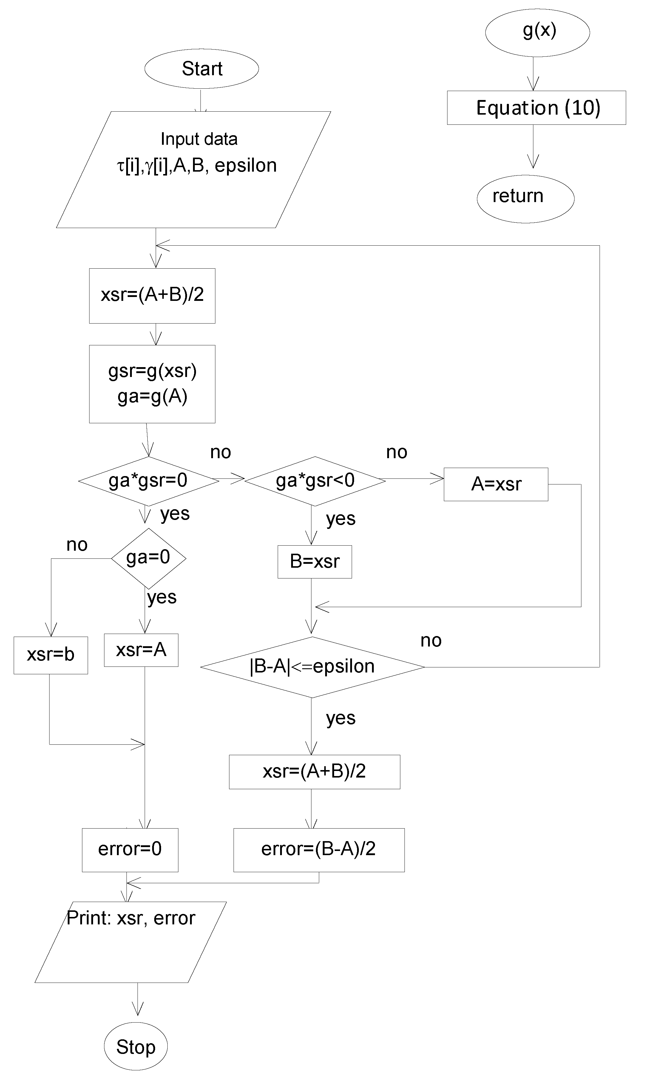
Due to the above, the Department of Drilling and Geoengineering, AGH University of Science and Technology in Kraków has developed a numerical program using the bisection method.

The algorithm for solving Equation (10), using the bisection method, is presented in Figure 1.

Given a determined value of the C parameter, other rheological parameters within the Vom Berg model can be specified from dependencies (11) and (12):

$$D=\frac{{\tau }_{600}-{\tau }_{300}}{sin{h}^{-1}\left(\frac{{\dot{\gamma }}_{600}}{C}\right)-sin{h}^{-1}\left(\frac{{\dot{\gamma }}_{300}}{C}\right)}$$

(11)

$${\tau }_y={\tau }_{600}-Dsin{h}^{-1}\left(\frac{{\dot{\gamma }}_{600}}{C}\right)$$

(12)

In the case of the Hahn–Eyring model, rheological parameters C, D, and E are determined by solving the system of equations:

$$\left\{\begin{array}{c}{\tau }_{600}=E{\dot{\gamma }}_{600}+D sin{h}^{-1}\left(\frac{{\dot{\gamma }}_{600}}{C}\right)\\ {\tau }_{300}=E{\dot{\gamma }}_{300}+D sin{h}^{-1}\left(\frac{{\dot{\gamma }}_{300}}{C}\right)\\ {\tau }_{200}=E{\dot{\gamma }}_{200}+D sin{h}^{-1}\left(\frac{{\dot{\gamma }}_{200}}{C}\right)\end{array}\right.$$

(13)

The value of the C parameter is acquired from a numerical solution of the equation:

$$\frac{\left(sin{h}^{-1}\left(\frac{{\dot{\gamma }}_{600}}{C}\right)-\frac{{\dot{\gamma }}_{600}}{{\dot{\gamma }}_{300}}sin{h}^{-1}\left(\frac{{\dot{\gamma }}_{300}}{C}\right)\right)}{\left(sin{h}^{-1}\left(\frac{{\dot{\gamma }}_{200}}{C}\right)-\frac{{\dot{\gamma }}_{200}}{{\dot{\gamma }}_{300}}sin{h}^{-1}\left(\frac{{\dot{\gamma }}_{300}}{C}\right)\right)}=\frac{{\tau }_{600}{\dot{\gamma }}_{300}-{\tau }_{300}{\dot{\gamma }}_{600}}{{\tau }_{200}{\dot{\gamma }}_{300}-{\tau }_{300}{\dot{\gamma }}_{200}}$$

(14)

To this end, assuming that x = C, the following function is constructed:

$$g\left(x\right)=\frac{\left(sin{h}^{-1}\left(\frac{{\dot{\gamma }}_{600}}{x}\right)-\frac{{\dot{\gamma }}_{600}}{{\dot{\gamma }}_{300}}sin{h}^{-1}\left(\frac{{\dot{\gamma }}_{300}}{x}\right)\right)}{\left(sin{h}^{-1}\left(\frac{{\dot{\gamma }}_{200}}{x}\right)-\frac{{\dot{\gamma }}_{200}}{{\dot{\gamma }}_{300}}sin{h}^{-1}\left(\frac{{\dot{\gamma }}_{300}}{x}\right)\right)}-\frac{{\tau }_{600}{\dot{\gamma }}_{300}-{\tau }_{300}{\dot{\gamma }}_{600}}{{\tau }_{200}{\dot{\gamma }}_{300}-{\tau }_{300}{\dot{\gamma }}_{200}}$$

(15)

Next, its zero is designated.

It is possible to use the algorithm presented formerly in Figure 1. Substituting, in the place of the g(x) function, a dependency (15), the value of parameter x = C is determined.

Given a calculated value of the C parameter, other rheological parameters within the Hahn–Eyring model should be specified from dependencies (16) and (17):

$$D=\frac{{\dot{\gamma }}_{300}{\tau }_{600}-{\tau }_{300}{\dot{\gamma }}_{600}}{{\dot{\gamma }}_{300}sin{h}^{-1}\left(\frac{{\dot{\gamma }}_{600}}{C}\right)-{\dot{\gamma }}_{600}sin{h}^{-1}\left(\frac{{\dot{\gamma }}_{300}}{C}\right)}$$

(16)

$$E=\frac{{\tau }_{300}-Dsin{h}^{-1}\left(\frac{{\dot{\gamma }}_{300}}{C}\right)}{{\dot{\gamma }}_{300}}$$

(17)

4. Determination of the Conditions of Shear Rate Measurements

Shear rates $\dot{\gamma }$ ∈ (511 s⁻¹ ÷ 1022 s⁻¹) are recognized as the basic conditions of a drilling fluid flow [3,8,26], which sometimes do not correspond to actual hydraulic conditions, since shear rates in the annular space of a borehole are lower. Thus, the application of the constant values of rheological parameters, determined for high shear rates, cannot be justified, from the practical point of view, in the case of flow characterized by low shear rates.

The need to take into account the influence of different flow conditions upon the value of drilling fluid rheological parameters makes it necessary to determine the rheological parameters of a given model separately for low shear rates and high shear rates [31].

In order to determine rheological parameters, it is not necessary to know the precise value of the shear rate occurring during a real fluid flow. The precise values of real shear rates of fluid can be determined only after establishing fluid rheological parameters. Apart from its rheological parameters, flow conditions such as a stream of flow volume and the geometry of an element in which flow takes place also have an impact on the real values of the shear rates of flowing drilling fluid. For a laminar flow of a Newtonian fluid through a pipe, the shear rate is determined as follows [8]:

$$\dot{\gamma }=\left(-\frac{dv}{dr}\right)=\frac{8v}{d_e}$$

(18)

This value is proposed to be assumed as the starting point for establishing the actual scope of shear rates for a non-Newtonian fluid. For drilling fluid flow rates and the geometry of drill pipes and drill collars used in the drilling practice, the shear rate determined from the Formula (18) is in the range $\dot{\gamma }$ ∈ (511 s⁻¹ ÷ 1022 s⁻¹) recommended by standard API 13 D. However, in case of flow through annular space (e.g., drill pipes—cased annular space) these values are much lower.

Therefore, it is suggested, before starting calculations, to determine shear rates from Formula (18) and take the value ${\dot{\gamma }}_{MID}\approx \frac{8v}{d_e}$ mostly approximated to it from the dependence of shear rates on rotational speeds of the external cylinder and shear stresses on the torsion angle of the external cylinder [20]. That value will define the range of shear rates, which should be considered when calculating drilling fluid rheological parameters ${\dot{\gamma }}_{MID}$ ∈ (${\dot{\gamma }}_{LOW}$ ÷ ${\dot{\gamma }}_{TOP}$). ${\dot{\gamma }}_{LOW}$ is a little smaller than the ${\dot{\gamma }}_{MID}$ shear rate recorded on a viscometer. ${\dot{\gamma }}_{TOP}$ is a little larger than the shear rate recorded on a viscometer.

When applying the abovementioned methodology, one can calculate fluid rheological parameters for any shear rate. It is then necessary to use dependencies (8) to (17) with the following substitutions, ${\dot{\gamma }}_{600}$ = ${\dot{\gamma }}_{TOP}$, ${\dot{\gamma }}_{300}$ = ${\dot{\gamma }}_{MID}$, ${\dot{\gamma }}_{200}$ = ${\dot{\gamma }}_{LOW}$, and respective measurement results, ${\tau }_{600}={\tau }_{TOP}$, ${\tau }_{300}={\tau }_{MID}$, ${\tau }_{600}={\tau }_{LOW}$.

The values of rheological parameters are then determined from the following dependencies:

• For the Vom Berg model:

$$\frac{sin{h}^{-1}\left(\frac{{\dot{\gamma }}_{TOP}}{C}\right)-sin{h}^{-1}\left(\frac{{\dot{\gamma }}_{MID}}{C}\right)}{sin{h}^{-1}\left(\frac{{\dot{\gamma }}_{TOP}}{C}\right)-sin{h}^{-1}\left(\frac{{\dot{\gamma }}_{LOW}}{C}\right)}=\frac{{\tau }_{TOP}-{\tau }_{MID}}{{\tau }_{TOP}-{\tau }_{LOW}}$$

(19)

$$D=\frac{{\tau }_{TOP}-{\tau }_{MID}}{sin{h}^{-1}\left(\frac{{\dot{\gamma }}_{TOP}}{C}\right)-sin{h}^{-1}\left(\frac{{\dot{\gamma }}_{MID}}{C}\right)}$$

(20)

$${\tau }_y={\tau }_{TOP}-D sin{h}^{-1}\left(\frac{{\dot{\gamma }}_{TOP}}{C}\right)$$

(21)

• For the Hahn–Eyring model:

$$\frac{\left(sin{h}^{-1}\left(\frac{{\dot{\gamma }}_{TOP}}{C}\right)-\frac{{\dot{\gamma }}_{TOP}}{{\dot{\gamma }}_{MID}}sin{h}^{-1}\left(\frac{{\dot{\gamma }}_{MID}}{C}\right)\right)}{\left(sin{h}^{-1}\left(\frac{{\dot{\gamma }}_{LOW}}{C}\right)-\frac{{\dot{\gamma }}_{LOW}}{{\dot{\gamma }}_{MID}}sin{h}^{-1}\left(\frac{{\dot{\gamma }}_{MID}}{C}\right)\right)}=\frac{{\tau }_{TOP}{\dot{\gamma }}_{MID}-{\tau }_{MID}{\dot{\gamma }}_{TOP}}{{\tau }_{LOW}{\dot{\gamma }}_{MID}-{\tau }_{MID}{\dot{\gamma }}_{LOW}}$$

(22)

$$D=\frac{{\dot{\gamma }}_{MID}{\tau }_{TOP}-{\tau }_{MID}{\dot{\gamma }}_{TOP}}{{\dot{\gamma }}_{MID}sin{h}^{-1}\left(\frac{{\dot{\gamma }}_{TOP}}{C}\right)-{\dot{\gamma }}_{TOP}sin{h}^{-1}\left(\frac{{\dot{\gamma }}_{MID}}{C}\right)}$$

(23)

$$E=\frac{{\tau }_{MID}-D sin{h}^{-1}\left(\frac{{\dot{\gamma }}_{MID}}{C}\right)}{{\dot{\gamma }}_{MID}}$$

(24)

5. Calculation of Correlations for Rheological Models of Reference Cement Slurry Samples According to API Standards

For the purposes of this article, laboratory tests were carried out in accordance with API standards [3,7,8,13,14,15] for unmodified fresh cement slurries. The water–cement ratio of the prepared cement slurries ranged from 0.38 to 0.56, depending on the depth of their application [13]. Viscosity measurements were performed with a Chan model 3500 viscometer according to API specifications [15]. The author’s Rheosolution methodology, described in detail [10], was used to compare the reference rheological models used in drilling practice and those recommended by API. 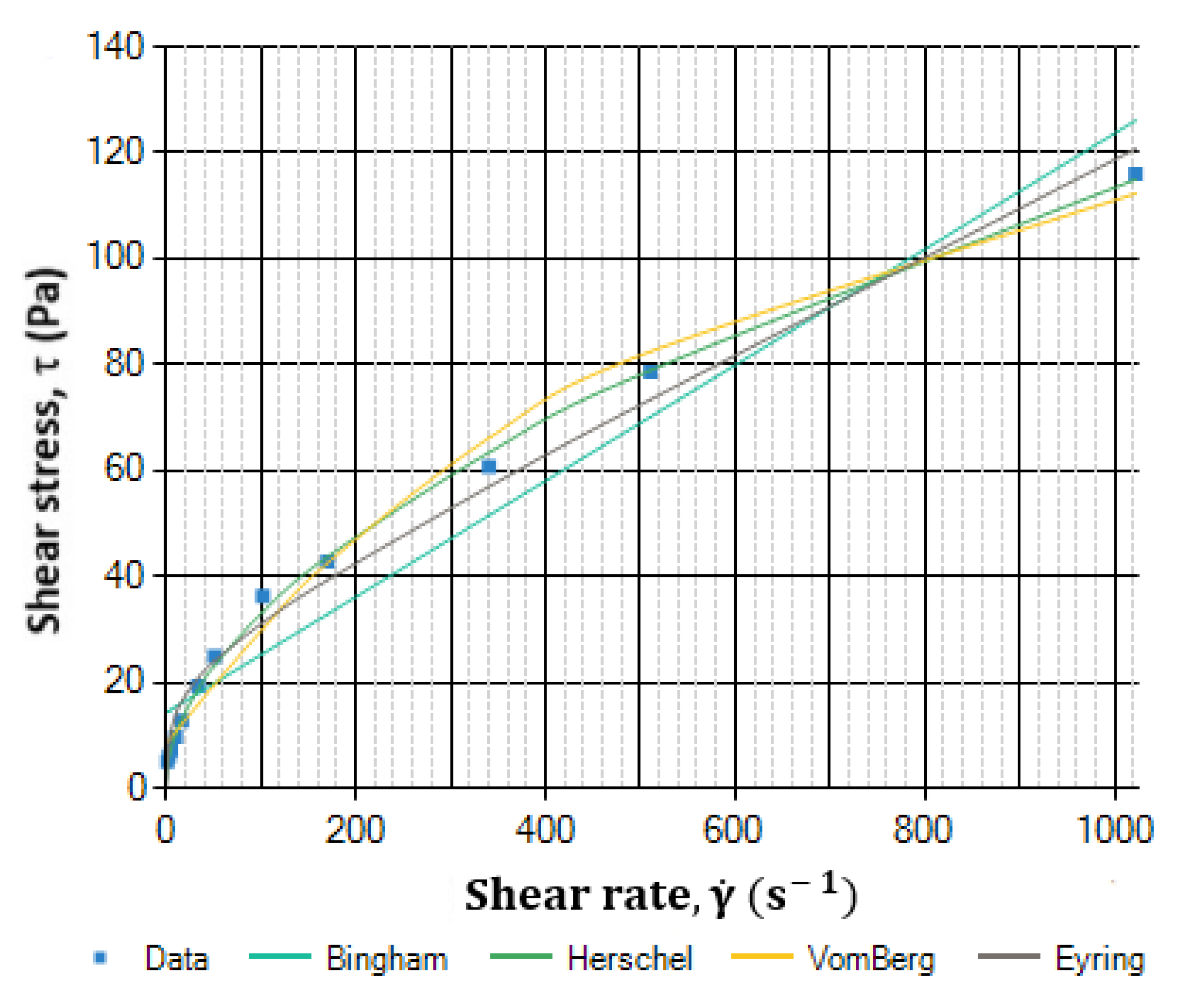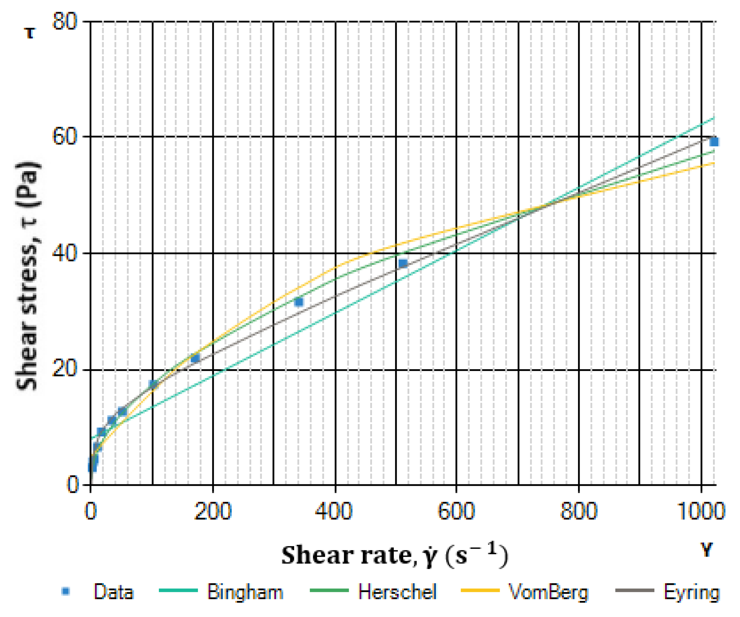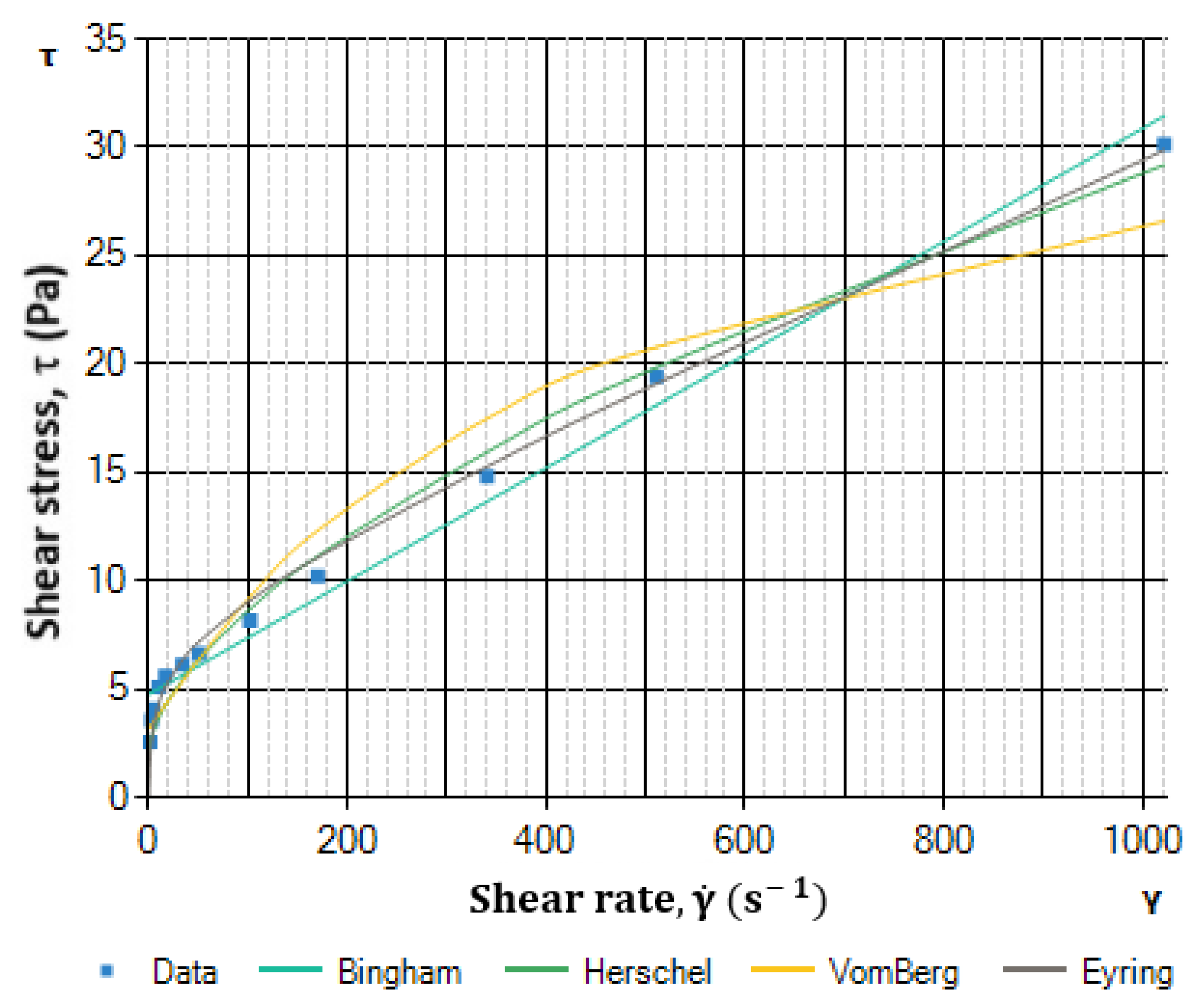In the laboratory tests, Class G cement was used [32]. The results are shown in

Table 1. Data from laboratory tests conducted on a Chan model 3500 viscometer (R1-B1, F1).

Cement w/c 0.38		Cement w/c 0.44		Cement w/c 0.46		Cement w/c 0.56
Rotations	Angle	Rotations	Angle	Rotations	Angle	Rotations	Angle
rot/min	°	rot/min	°	rot/min	°	rot/min	°
1	10	1	7	1	6	1	5
2	12	2	9	2	8	2	7
3	14	3	10	3	9	3	8
6	19	6	14	6	13	6	10
10	25	10	19	10	18	10	11
20	38	20	25	20	22	20	12
30	49	30	29	30	25	30	13
60	67	60	37	60	34	60	16
100	84	100	45	100	43	100	20
200	119	200	64	200	62	200	29
300	154	300	81	300	75	300	38
600	227	600	126	600	116	600	59

and

Table 2. Relations between shear stresses and shear rates obtained from laboratory tests on a Chan model 3500 viscometer (R1-B1, F1).

Cement w/c 0.38		Cement w/c 0.44		Cement w/c 0.46		Cement w/c 0.56
Shear Rate	Tension	Shear Rate	Tension	Shear Rate	Tension	Shear Rate	Tension
1/s	Pa	1/s	Pa	1/s	Pa	1/s	Pa
1.7034	5.107	1.7034	3.575	1.7034	3.064	1.7034	2.553
3.4068	6.128	3.4068	4.596	3.4068	4.085	3.4068	3.575
5.1102	7.149	5.1102	5.107	5.1102	4.596	5.1102	4.085
10.2204	9.703	10.2204	7.149	10.2204	6.639	10.2204	5.107
17.034	12.767	17.034	9.703	17.034	9.192	17.034	5.617
34.068	19.406	34.068	12.767	34.068	11.235	34.068	6.128
51.102	25.023	51.102	14.810	51.102	12.767	51.102	6.639
102.204	36.258	102.204	18.895	102.204	17.363	102.204	8.171
170.34	42.897	170.34	22.981	170.34	21.959	170.34	10.214
340.68	60.771	340.68	32.683	340.68	31.662	340.68	14.810
511.02	78.644	511.02	41.365	511.02	38.301	511.02	19.406
1022.04	115.924	1022.04	64.345	1022.04	59.239	1022.04	30.130

. The rheograms of selected rheological models are shown in Figure 2, Figure 3, Figure 4 and Figure 5.

The determined rheological parameters, using a methodology called Rheosolution, are summarized in

Table 3. Fluid rheological parameters obtained from Rheosolution for cement slurry reference samples.

		Cement w/c 0.38		Cement w/c 0.44
Newtonian	η = 0.13137	-	-	η = 0.88175	-	-
Bingham	ηpl = 0.10954	τy = 14.10289	-	ηpl = 0.05825	τy = 8.81906	-
Ostwald–de Waele	k = 3.31838	n = 0.50340	-	k = 2.63648	n = 0.44057	-
Casson	ηcas = 0.07894	τy = 5.87332	-	ηcas = 0.03739	τy = 4.42458	-
Herschel–Bulkley	k = 2.22463	n = 0.56905	τy = 1.24404	k = 1.46080	n = 0.53840	τy = 1.23165
Vom Berg	τy = 8.13975	D = 44.16195	C = 196.78490	τy = 6.27191	D = 26.11636	C = 249.3056
Hahn–Eyring	E = 0.08843	D = 3.89513	C = 0.78079	E = 0.04385	D = 2.64770	C = 1.02734

and

Table 4. Fluid rheological parameters obtained from Rheosolution for cement slurry reference samples.

		Cement w/c 0.46		Cement w/c 0.56
Newtonian	η = 0.88156	-	-	η = 0.03348	-	-
Bingham	ηpl = 0.05414	τy = 8.10671	-	ηpl = 0.02610	τy = 4.7683	-
Ostwald–de Waele	k = 2.31330	n = 0.45098	-	k = 2.10455	n = 0.34045	-
Casson	ηcas = 0.03553	τy = 3.94491	-	ηcas = 0.0139	τy = 2.95886	-
Herschel–Bulkley	k = 1.35818	n = 0.53800	τy = 1.19420	k = 0.40279	n = 0.60791	τy = 1.99937
Vom Berg	τy = 5.01232	D = 20.56962	C = 175.6679	τy = 3.17826	D = 8.53888	C = 132.1473
Hahn–Eyring	E = 0.04100	D = 2.39472	C = 0.94129	E = 0.01930	D = 1.31098	C = 0.89122

.

Table 5. Results of the rheological model selection obtained from Rheosolution for cement slurry samples.

	Cement w/c 0.38			Cement w/c 0.44
Model/Coefficient	R	F	U	R	F	U
Newtonian	0.90357	44.47801	59.73121	0.88175	34.94199	817.2551
Bingham	0.97196	170.85500	2.78326	0.97837	223.69170	157.16900
Ostwald–de Waele	0.99750	1989.78700	22.11583	0.98857	429.79860	83.51331
Casson	0.98680	371.41910	1.34393	0.99325	733.50620	49.40012
Herschel–Bulkley	0.99925	6618.16700	3.02866	0.99660	1464.4270	24.91083
Vom Berg	0.99441	887.19650	32.89705	0.99079	535.25650	67.36108
Hahn–Eyring	0.99414	845.21680	153.87890	0.99933	7403.7060	4.95413

and

Table 6. Results of the rheological model selection obtained from Rheosolution for cement slurry samples.

	Cement w/c 0.46			Cement w/c 0.56
Model/Coefficient	R	F	U	R	F	U
Newtonian	0.88156	34.87228	710.9619	0.84389	24.74113	207.3356
Bingham	0.97569	198.23410	153.2048	0.98998	491.2643	14.3698
Ostwald–de Waele	0.99227	639.28060	49.13534	0.94567	84.60614	76.1376
Casson	0.99164	590.56980	53.12027	0.99622	1717.667	6.56551
Herschel–Bulkley	0.99817	2722.0010	11.67705	0.99335	744.6800	9.54449
Vom Berg	0.99153	582.5728	53.83714	0.97743	214.0158	32.1544
Hahn–Eyring	0.99836	3043.2340	10.44849	0.99652	1728.339	5.00788

summarize the correlation coefficients and Fischer–Snedecor statistical coefficients for the cement slurries tested. The best-fit model for a particular drilling cement sample is indicated.

From the above studies, it can be seen that the Vom Berg and especially the Hahn–Eyring rheological models show a very high correlation for the reference cement slurries. The Hahn–Eyring model shows the highest correlation for samples prepared at water/cement ratios of 0.44, 0.46, and 0.56. The differences from the Herschel–Bulkley model are not large and it can be concluded that these models for these cement slurry samples are comparable for practical applications in flow resistance calculations.

6. Practical Application of Calculated Dependencies for the Vom Berg and Hahn–Eyring Models

In order to exemplify the developed dependencies, rheological models for drilling mud pumped to drill pipes and pumped out to the annular space were developed, with a stream of flow volume Q = 0.03 m³/s. Rheological models were determined for mud flowing:

• Through drill pipes with the external diameter of 31/2″ (internal diameter: d_{I_PIPE} = 0.0702 mm, external diameter: d_{E_PIPE} = 0.0889 mm);
• Between 31/2″ drill pipes and 95/8″ casings (internal diameter: d_{I_CAS} = 0.2244 mm, external diameter: d_{E_CAS} = 0.2445 mm).

By means of a rotational viscometer, type Fann model 35A/SR-12 (in the arrangement R1-B1 and the applied spring F1), the rheological properties of the cement slurry to be used in a borehole were measured. The measurement results of torsion angles of the external cylinder (Φ), read for the setpoint rotational speeds (n), are presented in Table 5. By means of dependencies (6) and (7), the shear stresses (τ) and shear rates $\left({\dot{\gamma }}_i\right)$ occurring during measurements were calculated. The calculation results have been also provided in Table 5.

Next, on the basis of the developed methodology, the rheological parameters of the tested fluid were determined, taking the Vom Berg and Hahn–Eyring models as the rheological models of that fluid.

For this purpose, approximated shear rate inside a 3¹/₂″ drill pipe ($\dot{\gamma }\approx 883.3 {\mathrm{s}}^{-1}$) and in the annular space between 3¹/₂″ drill pipes and 9⁵/₈″ casings ($\dot{\gamma }\approx 122.8 {\mathrm{s}}^{-1}$) were estimated by means of Equation (18). Those values were used to estimate values ${\dot{\gamma }}_{LOW}$, ${\dot{\gamma }}_{MID}$, and ${\dot{\gamma }}_{TOP}$ for each space being analyzed. The results of laboratory tests and calculations have been also presented in

Table 7. Results of laboratory measurements and calculations of shear stresses and shear rates for the tested drilling mud in a 12-speed Fann viscometer 35A/SR-12, with the arrangement of cylinders R1-B1 and spring F1.

Laboratory Measurement
Rotational speed n, [RPM]	0.9	1.8	3	6	30	60	90	100	180	200	300	600
Torsion angle Φ, [-]	23	24	26	28	31	35	38	45	52	65	76	98
Calculated values
$\mathrm{Shear}\mathrm{rate}\dot{\gamma }$, [s−1]	1.53	3.07	5.11	10.22	51.10	102.20	153.31	170.34	306.61	340.68	511.02	1022.04
Shear stresses τ, [Pa]	11.75	12.26	13.29	14.31	15.84	17.89	19.42	23.00	26.06	33.22	38.84	50.08

and

Table 8. Results of calculations with regard to the rheological parameters of the tested drilling mud.

Interior of 31/2″ Drill Pipes
Shear rate $\dot{\gamma }$, [s−1] $\dot{\gamma }\approx 883.3 {\mathrm{s}}^{-1}$		${\dot{\gamma }}_{LOW}$		${\dot{\gamma }}_{MID}$		${\dot{\gamma }}_{TOP}$
		340.48		511.02		1022.04
Shear stresses τ, [Pa]		${\tau }_{LOW}$		${\tau }_{MID}$		${\tau }_{TOP}$
		33.22		38.84		50.08
Vom Berg model				Hahn–Eyring model
τy	D		C	E	D		C
17.55255355	18.10492882		348.6600	0.00732346	10.83764167		40.1643
Annular space 31/2″–95/8″
$\mathrm{Shear}\mathrm{rate}\dot{\gamma }$, [s−1] $\dot{\gamma }\approx 122.8 {\mathrm{s}}^{-1}$		${\dot{\gamma }}_{LOW}$		${\dot{\gamma }}_{MID}$		${\dot{\gamma }}_{TOP}$
		51.10		102.02		153.31
Shear stresses τ, [Pa]		${\tau }_{LOW}$		${\tau }_{MID}$		${\tau }_{TOP}$
		19.42		23		26.06
Vom Berg model				Hahn–Eyring model
τy	D		C	E	D		C
13.25003780	4.59896869		86.080000	0.01590531	1.77624900		0.021630

.

Assuming the Vom Berg model, a rheological equation of drilling fluid is obtained:

• In the case of flow through 3¹/₂″ drill pipes:

$$\tau =17.553+18.105\cdot sin h^{-1}\left(\frac{-\frac{dv}{dr}}{348.66}\right)$$

(25)

• In the case of flow through 3½″–9⁵/₈″ annular space:

$$\tau =13.25+4.599\cdot sin h^{-1}\left(\frac{-\frac{dv}{dr}}{86.08}\right)$$

(26)

Taking the Hahn–Eyring model, a rheological equation for drilling fluid is obtained:

• In the case of flow through 3¹/₂″ drill pipes:

$$\tau =0.0073\left(-\frac{dv}{dr}\right)+10.838\cdot sin h^{-1}\left(\frac{-\frac{dv}{dr}}{40.164}\right)$$

(27)

• In the case of flow through 3½″–9⁵/₈″ annular space:

$$\tau =0.0159\left(-\frac{dv}{dr}\right)+1.776\cdot sin h^{-1}\left(\frac{-\frac{dv}{dr}}{0.0216}\right)$$

(28)

7. Conclusions

Various process fluids are used in drilling practice, such as drilling muds with various additives, affecting a change in rheological parameters [33], drill-in fluids, fracturing fluids, spacers, washes, and cement slurries. They are an important element of drilling technology and accurate knowledge of their flow parameters results in better control of the entire drilling process.

Technological fluids used in drilling are non-Newtonian fluids, described by rheological models: Bingham plastic, power law, or yield power law. These rheological models recommended by the API for some technological drilling fluids show much less correlation, and consequently, the flow resistance calculations can have large errors. This can have consequences related to the safety of drilling operations and economic aspects, such as the overestimation of mud pumps or cementing units.

The behavior of the actual drilling fluid is most accurately approximated by three-parameter models, therefore it is proposed to use the Vom Berg and Hahn–Eyring three-parameter models, which have not yet been used in the drilling industry, in addition to the Herschel–Bulkley model. The strong correlation of these models with real drilling fluids means that the calculated flow resistances will be close to the real ones and decisions related to the selection of appropriate pumps for drilling investments will be close to optimal. The author’s methodology for selecting the optimum rheological model, called Rheosolution, described in detail in paper [10], makes it possible to effectively determine the parameters of these rheological models for drilling fluids.

The selection of a rheological model for drilling fluids should be closely related to the application conditions of the drilling fluid (flow geometry and hydraulic parameters used).

The rheological parameters of drilling muds and cement slurries for the Vom Berg and Hahn Eyring models should be determined from the equations derived and presented in this paper. To simplify this, the software Rheosolution v 4.0 [10] was developed to support engineering decisions in this field, reducing to a minimum the time needed to determine the rheological parameters of three-parameter models, which is important in industrial practice. The above methodology can be integrated with real-time rheological parameter measurement systems [34] and the rheological models in question can be used to accurately determine the flow parameters of polymer-modified deepwater drilling fluids [35] or drilling muds with solid contents [36].

References

1. Toczek, P.; Wiśniowski, R.; Stryczek, S.; Ziaja, J.; Mazur, C. Total Specific Energy (TSE) as a New Indicator of Drilling Efficiency. AGH Drill. Oil Gas 2017, 34, 715–729. [Google Scholar]
2. Wiśniowski, R.; Toczek, P. Minimizing Bottomhole Pressure Losses USING TSE–Total Specific Energy–A New Indicator of Drilling Efficiency. In Proceedings of the 18th International Multidisciplinary Scientific GeoConference SGEM, Albena, Bulgaria, 2–8 July 2018. [Google Scholar]
3. API RP 13D; Rheology and Hydraulics of Oil-Well Drilling Fluids. American Petroleum Institute, API: Dallas, TX, USA, 2017. Available online: https://standards.globalspec.com/std/10180185/api-rp-13d (accessed on 2 June 2022).
4. Polska Norma BN-90/1785-01; Płuczka Wiertnicza. Metody badań w Warunkach Polowych. Wydawnictwa Normalizacyjne ALFA: Warszawa, Poland, 1990.
5. Wiśniowski, R. Metodyka określania modelu reologicznego cieczy wiertniczej. Wiert. Naft. Gaz 2001, 18, 247–261. [Google Scholar]
6. Wiśniowski, R. Zastosowanie Modelu Herschel-Bulkleya w Hydraulice Płuczek Wiertniczych; Nowoczesne Techniki i Technologie Bezwykopowe: Kraków, Poland, 2000. [Google Scholar]
7. Mitchell, R.F.; Miska, S.Z. Fundamentals of Drilling Engineering. In SPE Textbook; Society of Petroleum Engineers: Richardson, TX, USA, 2011; Volume 12. [Google Scholar]
8. Bourgoyne, A.T.; Milheim, K.K.; Chenevert, M.E.; Young, F.S. Applied Drilling Engineering. In SPE Textbook; Society of Petroleum Engineers: Richardson, TX, USA, 1986. [Google Scholar]
9. Vom Berg, W. Influence of specific surface and concentration of solids upon the flow behaviour of cement pastes. Mag. Concr. Res. 1979, 31, 211–216. [Google Scholar] [CrossRef]
10. Wiśniowski, R.; Skrzypaszek, K.; Małachowski, T. Selection of Suitable Rheological Model for Driling Fluid Using Applied Numerical Methods. Energies 2020, 13, 3192. [Google Scholar] [CrossRef]
11. Lapasin, R.; Papo, A.; Rajgelj, S. The phenomenological description of the thixotropic behaviour of fresh cement pastes. Rheol. Acta 1983, 22, 410–416. [Google Scholar] [CrossRef]
12. Papo, A. Rheological models for cement pastes. Mater. Struct. 1988, 21, 41–46. [Google Scholar] [CrossRef]
13. Stryczek, S. Poradnik Górnika Naftowego; Stowarzyszenie Naukowo-Techniczne Inżynierów i Techników Przemysłu Naftowego i Gazowniczego: Krakow, Poland, 2015; pp. 723–726. [Google Scholar]
14. API Specification 10A, 10B. Cements and Materials for Well Cementing, 25th ed.; 2019; Available online: https://standards.globalspec.com/std/14208303/api-spec-10a (accessed on 20 May 2022).
15. American Petroleum Institute. Specification for Materials and Testing for Well Cements, 5th ed.; API Spec. 10; American Petroleum Institute: Dallas, TX, USA, 1990. [Google Scholar]
16. Mezger, T.G. The Rheology Handbook For Users of Rotational and Oscillatory Rheometers; Hanover Vincenzt Network: Hanover, Germany, 2006. [Google Scholar]
17. Bair, S. Actual Eyring Models for Thixotropy and Shear-Thinning: Experimental Validation and Application to EHD. J. Tribol. 2004, 126, 728–732. [Google Scholar] [CrossRef]
18. Benyounes, K. Rheological behavior of cement-based grout with Algerian bentonite. SN Appl. Sci. 2019, 1, 1037. [Google Scholar] [CrossRef] [Green Version]
19. OFITE. OFI Testing Equipment Inc. Product Catalog. Drilling Fluids, Cement, Core Analysis, Laboratory Supplies Reagents; OFI Testing Equipment Inc.: Houston, TX, USA, 2017. [Google Scholar]
20. Manual No. 208878; Model 35 Instruction Manual. 2016 Fann Instrument Company: Houston, TX, USA, 2016.
21. Brookfield Viscometers/Rheometers; Catalogue of Brookfield Company: Middleboro, MA, USA, 1999.
22. Haake Series 1; Thermo Fisher Scientific Inc. Materials: Hanover, Germany, 2018.
23. Haake: Material Characterisation & Testing Products; Rheology Solution Victoria Company Materials: Victoria, Australia, 2019.
24. OFI Testing Equipment, Inc. Testing Equipment for Drilling Fluids, Cement, Core; OFI Testing Equipment, Inc.: Houston, TX, USA, 2017. [Google Scholar]
25. Klotz, J.A.; Brigham, W.E. To determine Herschel-Bulkley coefficients. J. Pet. Technol. 1998, 50, 80–81. [Google Scholar] [CrossRef]
26. Pellegrino, C.; Faleshini, F. Sustainability Improvements in the Concrete Industry: Use of Recycled Materials for Structure Concrete Production; 2016-Technology & Engineering; Springer International Publishing: Cham, Switzerland, 2016. [Google Scholar]
27. Ahmad, A.G. Comparative Study of Bisection and Newton-Rhapson Methods of Root-Finding Problems. Int. J. Math. Trends Technol. 2015, 19, 121–129. [Google Scholar] [CrossRef]
28. Dalquist, G.; Biorck, A. Numerical Methods; Dower Publication Inc.: Mineula, NY, USA, 2003. [Google Scholar]
29. Ehiwario, J.C.; Aghamie, S.O. Comparative Study of Bisection, Newton-Raphson and Secant Methods of Root-Finding Problems. IOSR J. Eng. 2014, 4, 1–7. [Google Scholar]
30. Azure, I.; Aloliga, G.; Doabil, L. Comparative Study of Numerical Methods for Solving Non-linear Equations Using Manual Computation. Math. Lett. 2019, 5, 41–46. [Google Scholar] [CrossRef]
31. Hoechst Polymer Fluids; Company Information Materials: Hoechst, Germany, 1989.
32. Rzepka, M.; Kedzierski, M. Cement Slurries for Sealing Boreholes in the Polish Lowlands in Difficult Geological and Technical Conditions; Nafta-Gaz 2020; Oil and Gas Institute—National Research Institute, INiG: Kraków, Poland, 2020; pp. 91–100. [Google Scholar] [CrossRef]
33. Medved, I.; Gaurina-Međimurec, N.; Novak Mavar, K.; Mijić, P. Waste Mandarin Peel as an Eco-Friendly Water-Based Drilling Fluid Additive. Energies 2022, 15, 2591. [Google Scholar] [CrossRef]
34. Liu, N.; Zhang, D.; Gao, H.; Hu, Y.; Duan, L. Real-Time Measurement of Drilling Fluid Rheological Properties: A Review. Sensors 2021, 21, 3592. [Google Scholar] [CrossRef] [PubMed]
35. Wang, Z.; Sun, J.; Zhang, K.; Lv, K.; Huang, X.; Wang, J.; Wang, R.; Meng, X. A Temperature-Sensitive Polymeric Rheology Modifier Used in Water-Based Drilling Fluid for Deepwater Drilling. Gels 2022, 8, 338. [Google Scholar] [CrossRef] [PubMed]
36. Leusheva, E.; Brovkina, N.; Morenov, V. Investigation of Non-Linear Rheological Characteristics of Barite-Free Drilling Fluids. Fluids 2021, 6, 327. [Google Scholar] [CrossRef]
Figure 1. Flow chart for the calculation of the root of the g(x) function being in the range (A,B) by means of the bisection method.
Energies 15 05583 g001
Figure 2. Comparison of the selected rheological models, cement w/c 0.38.
Energies 15 05583 g002
Figure 3. Comparison of the selected rheological models, cement w/c 0.44.
Energies 15 05583 g003
Figure 4. Comparison of the selected rheological models, cement w/c 0.46.
Energies 15 05583 g004
Figure 5. Comparison of the selected rheological models, cement w/c 0.56.
Energies 15 05583 g005