Experiment and Numerical Simulation on Hydraulic Loss and Flow Pattern of Low Hump Outlet Conduit with Different Inlet Water Rotation Speeds

Abstract

The rotation speed of water at the inlet of the low hump outlet conduit has a great effect on its hydraulic performance. Therefore, the influence of different inlet water rotation speeds on hydraulic loss and flow pattern of low hump outlet conduit is studied in this paper. By solving RANS equations and the RNG k-ε turbulence model, the hydraulic loss and 3D flow field of the low hump outlet conduit were calculated under different inlet water rotation speeds. To verify the numerical results, the model tests of low hump outlet conduit with different guide vanes were conducted. The results show that along with the growth of inlet water rotation speed, the hydraulic loss of outlet conduit will firstly decrease by degrees and then increase dramatically, the vortex location moves from the whole bottom of the descent segment to the right bottom of descent segment and the vortex area becomes smaller, the flow pattern of the whole conduit is improved obviously. The hydraulic loss and flow field of numerical simulation are consistent with those of the model test. Because of its great influence on hydraulic performance, inlet water rotation speed must be taken into consideration in the hydraulic optimization design of guide vane and low hump outlet conduit.

1. Introduction

An axial flow pumping station with low head and mass flow is widely applied in numerous spheres such as interbasin water diversion, irrigation and drainage, urban flood control, and so on. As an essential component of an axial flow pump device in a large pump station, the outlet conduit, located between the guide vane and outlet sump, plays the role of transforming fluid kinetic energy into pressure energy so as to reduce hydraulic loss [1]. Significantly, the hydraulic loss including the route loss and local loss caused by outlet conduit accounted for a large proportion of the head of the pump device, and then exerted a strong influence on the efficiency of the pump device [2,3,4]. Therefore, the research on the hydraulic performance of outlet conduits should be especially emphasized.

The hydraulic performance of pipe is affected by many common factors such as cavitation, inlet water rotation speed, etc. For cavitation, Ge et al. [5,6,7,8] studied the effect of temperature on the hydraulic cavitation dynamics in a small Venturi channel, the results indicated that different cavitation characteristics would influence the hydraulic performance of the pipe. In addition, the inlet water rotation speed of pipe is another key factor affecting the hydraulic performance of pipe and will be studied in detail. McDonald et al. [9] studied the influence of swirl inlet flow on conical diffusers by experimentation, the results indicated that the swirl inlet water would improve the hydraulic performance of conical diffusers. Prakash et al. [10] studied the influence of swirl inlet flow on conical diffusers by numerical simulation, the results indicated that the flow swirl number value played an important role in the hydraulic performance of conical diffusers and the hydraulic performance of conical diffusers would be improved in a certain flow swirl value. Kaya et al. [11] studied the tangential velocity energy of an axial pump by experimentation, the results indicated the axial pump with a guide vane had a better hydraulic performance compared with the axial pump without a guide vane because the guide vane changed the tangential velocity of swirl flow. Susan-Resiga et al. [12] studied the swirl flow in the draft tube bend of the Francis turbine, the results indicated the critical swirl should be avoided so as to achieve higher hydraulic performance. The above studies indicated that the hydraulic performance of pipe would be improved with a certain swirl flow and this improvement was applied in the axial pump and Francis turbine. In a pump device with a low head, the fluid from the guide vane still possessed a certain degree of residual circulation [13], which resulted in the flow having a certain tangential velocity when flowing into the outlet conduit. The results of the model test indicated that the fluid tangential velocity at the exit section of the guide vane measured in the design condition basically showed a linear distribution from hub to flange [14]. Qiu et al. [15,16] studied the flow pattern of outlet conduit in an axial flow pump system, the results indicated that complex flow and non-uniform distribution of section velocity took place in outlet conduit on account of flow rotation at the exit section of guide vane and brought out the diverse flow rate in the left and right hole of outlet conduit. Zhu et al. [17,18] studied the hydraulic performance of siphon outlet conduit in the different operating conditions of an axial flow pump, and the research results revealed that the relationship between hydraulic loss and discharge was inconsistent with the second-order parabolic law on account of residual circulation at the outlet of guide vane. Cai [19] used a numerical simulation method to study the relationship between hydraulic loss or pressure recovery coefficient and discharge in siphon outlet conduit and straight pipe outlet conduit under disparate operating conditions. Liang et al. [14] studied the hydraulic loss of siphon outlet conduit and low hump outlet conduit under diverse guide vane outlet circulation, and the results indicate that the circulation, which minimizes hydraulic loss, exists. The above studies indicate that the hydraulic loss and flow pattern of the outlet conduit are affected by the rotation of the water at the outlet cross-section of the guide vane, namely, the inlet cross-section of the outlet conduit.

Low hump outlet conduits are extensively adopted in vertical axial flow pumping stations, and moreover, seven of the fourteen vertical pumping stations with low heads have used the low hump outlet conduit in the first-stage Project of Eastern Route of South-to-North Water Diversion [1]. The project diverts the Yangtze River water from southern China to the north through low-head pumping stations and river channels [20]. Previous studies indicated that residual circulation at the exit section of the guide vane had an influence on the hydraulic performance of outlet conduit, but in these studies, the main type of outlet conduit was a siphoned outlet conduit. In the reference [14], the analysis of flow pattern in outlet conduit under different inlet water rotation speeds was not researched for the low hump outlet conduit. The design parameters of low hump outlet conduit in the research [14] were as follows: length of conduit 18,000 mm, the diameter of inlet section 2800 mm, the width of outlet section 7000 mm, the height of outlet section 3500 mm, the length of inlet transition segment 6890 mm, the height of inlet transition segment 4260 mm, and the diffusion angle of plane 12°. There are multiple parameters including length of conduit, length, and height of transition segment, boundary line shape of conduit, and diffusion angle of the plane that have an effect on the hydraulic performance of low hump outlet conduit [21]. If the design parameters of the outlet conduit are different from those in research [21], will the variation rule of outlet conduit hydraulic performance be changed under different inlet water rotation speeds?

The Computational Fluid Dynamics (CFD) method is used more and more in the field of hydraulic engineering research. Wang et al. [22] studied the effects of the impeller blade with a slot structure on the centrifugal pump performance using the numerical simulation method. Luo et al. [23] predicted the energy performance curve of centrifugal pumps. Zhou et al. [24] studied the pressure fluctuations characteristics in a centrifugal pump by the method of numerical simulation. Sun et al. [25] studied the hydraulic performance and flow patterns of axial-flow pumps with axial stacking of different airfoil series based on Navier–Stokes equations and the SST k-w turbulence model. Song et al. [26] used the numerical simulation method to research pressure pulsation characteristics of nuclear coolant pumps under different boundary conditions. Xu et al. [27] used the RNG k-ε turbulence model to calculate the hydraulic characteristic of outlet conduit in a pump system with a slanted extension shaft under the conditions of different middle pier lengths. Jiang et al. [28] studied the hydraulic characteristics of a three-side inlet of vertical shaft inlet channel of a horizontal pumping station based on the Navier–Stokes equations and RNG k-ε turbulence model. Tong et al. [29] used the CFD method to study the hydrodynamic performance of slanted axial-flow urban drainage pumps under shut-off conditions. Lu et al. [30] compared the hydraulic performance of submersible tubular pump devices with motor front and rear arrangements by the CFD method. Shi et al. [31] analyzed the effect of blade angle on hydraulic performance for pumping system of water diversion pumping station based on the incompressible Navier–Stokes equations and an RNG k-ε turbulence model. Teuber et al. [32] studied the CFD-modeling of free surface flows in closed conduits based on the open-source software OpenFOAM (OpenCFD Ltd., Reading, UK). Simao et al. [33] used the CFD method to analyze the velocity profiles in a pump as a turbine and verified by the ultrasonic doppler velocimetry. Rezvaya et al. [34] used CFD programs to solve the hydrodynamical tasks on the example of the bulb-type turbine, the reversible hydraulic machine, and the centrifugal submersible pump. Gunjo et al. [35] investigated the absorber plate and outlet water temperature of a solar flat plate collector with a straight riser and header arrangement using a three-dimensional CFD. Seyedashraf et al. [36] did a three-dimensional CFD study of free-surface flow in a sharply curved 30 open-channel bend. Ziaei et al. [37] studied the flow around a triangular labyrinth side weir with three different included angles (45°, 60°, and 90°). The CFD method also has been widely used in the studies of sewage pumps [38], hydroturbine [39], and other aspects [40,41].

In this paper, a low hump outlet conduit whose design parameters are different from the outlet conduit in reference [14] was selected as the study object, and the effect of inlet water rotation speed on the hydraulic performance of a low hump outlet conduit was studied by numerical simulation of 3D turbulent flow. Furthermore, the change in hydraulic loss and flow pattern in low hump outlet conduit are analyzed under different inlet water rotation speeds, and numerical simulation results are validated by model test results.

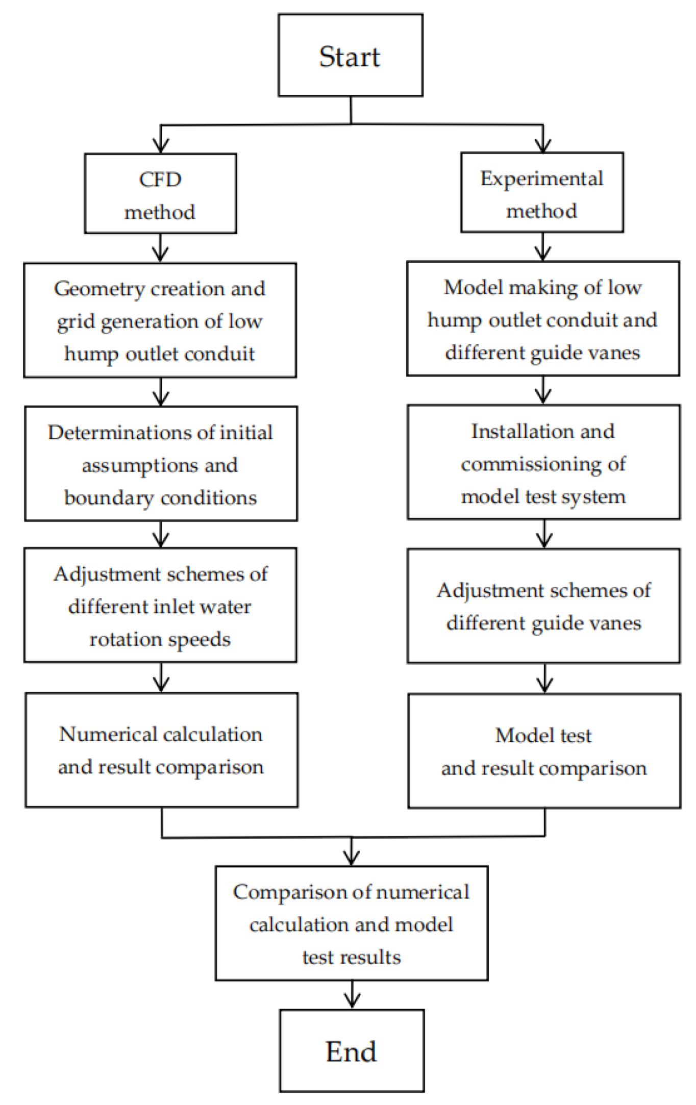
2. Research Object and Method

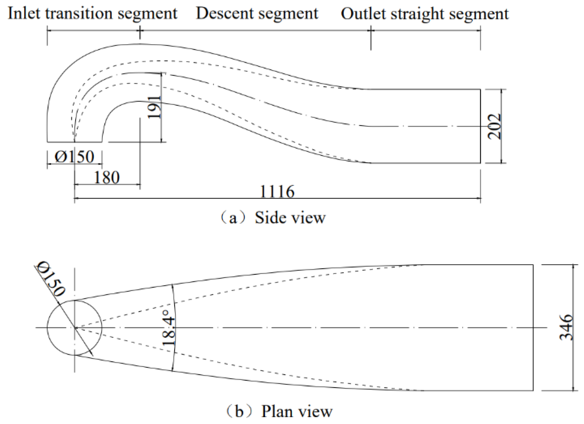
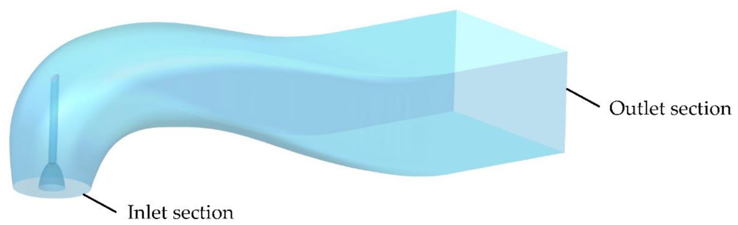
2.1. Geometrical Parameters and Research Methods

A vertical axial flow pump device is adopted in a pump station with a low head in the first-stage Project of Eastern Route of South-to-North Water Diversion. In this pump device, the design flow of a single pump is 33.5 m³/s, TJ04-ZL-06 of the pump models in South-to-North Water Diversion tested on the same test bed is chosen, pump impeller diameter is 3150 mm, elbow inlet conduit and low hump outlet conduit are chosen. Design parameters of this prototype conduit are as follows: length of outlet conduit 24,850 mm, the diameter of inlet section 3339 mm, the width of outlet section 7700 mm, the height of outlet section 4500 mm, length of inlet transition segment 4000 mm, the height of inlet transition segment 4250 mm and diffusion angle of plane 18.4°. For carrying out the model test, the prototype outlet conduit is proportionally scaled down and the inlet section diameter of the model outlet conduit is 150 mm. The detailed geometrical parameters of the model low hump outlet conduit are shown in

Table 1. Detailed geometrical parameters of model low hump outlet conduit.

Parameter	Value
Diameter of inlet section (mm)	150
Length of outlet conduit (mm)	1116
Length of inlet transition segment (mm)	180
Height of inlet transition segment (mm)	191
Diffusion angle of plane (°)	18.4
Width of outlet section (mm)	346
Height of outlet section (mm)	202

. The single-line diagram and 3D model diagram of the model low hump outlet conduit is, respectively, shown in Figure 1 and Figure 2, which are grouped into inlet transition segment, descent segment, and outlet straight segment according to the character of the outlet conduit. The cross-sectional shape of the low hump outlet conduit is gradually changed from a circular shape at the inlet section to a rectangular shape at the outlet section.

In this research, CFD and experimental methods were used to study the effect of inlet water rotation speed on the hydraulic loss and flow pattern in low hump outlet conduit. The flowchart is shown in Figure 3.

2.2. Mathematical Model and Numerical Computational Method

2.2.1. Mathematical Model

The flow of water in a low hump outlet conduit can be described by the conservation of mass equation and conservation of momentum equation (Navier–Stokes equation). In addition, the water in the low hump outlet conduit is incompressible ($\rho =\mathrm{constant}$) because the pressure in the outlet conduit is not high. Thus, two equations are simplified as below:

$$\frac{\partial u_i}{\partial x_i}=0$$

(1)

$$\rho \frac{\partial u_i}{\partial t}+\rho \frac{\partial u_i{u}_j}{\partial x_j}=-\frac{\partial p}{\partial x_i}+\frac{\partial }{\partial x_j}\left[\mu \left(\frac{\partial u_i}{\partial x_j}+\frac{\partial u_j}{\partial x_i}\right)\right]+F_i$$

(2)

where $u_i$,$u_j$ are velocity component; $x_i$,$x_j$ are coordinate direction; $t$ is time; $p$ is pressure; $\mu$ is coefficient of dynamic viscosity; $F_i$ is gravity force.

The Navier–Stokes equation is difficult to be solved directly. Thus, the Reynolds Average Navier–Stokes equation is introduced to describe turbulent flow, the transient turbulent flow is disassembled as the superposition of time-averaged flow and transient fluctuation flow. The transient variables, $u_i$ and $p$, are defined as below:

$$u_i={\overline{u}}_i+{u_i}^{\prime }$$

(3)

$$p=\overline{p}+p^{\prime }$$

(4)

where ${\overline{u}}_i$ is time-averaged velocity component; ${u_i}^{\prime }$ is fluctuant velocity component; $\overline{p}$ is time-averaged pressure; $p^{\prime }$ is fluctuant pressure.

After putting the Equations (3) and (4) into Equations (1) and (2), the governing equations of time-averaged turbulent flow are as flow:

$$\frac{\partial \overline{u_i}}{\partial x_i}=0$$

(5)

$$\rho \frac{\partial \overline{u_i}}{\partial t}+\rho \frac{\partial \overline{u_i}\overline{u_j}}{\partial x_j}=-\frac{\partial \overline{p}}{\partial x_i}+\frac{\partial }{\partial x_j}\left[\mu \left(\frac{\partial \overline{u_i}}{\partial x_j}+\frac{\partial \overline{u_j}}{\partial x_i}\right)-\rho \overline{u_i^{\prime }{u}_j^{\prime }}\right]+F_i$$

(6)

where $-\rho \overline{u_i^{\prime }{u}_j^{\prime }}$ is Reynolds stress.

To close the time-averaged equations, Boussinesq approximation is introduced to represent Reynolds stress as a function of turbulent viscosity ${\mu }_t$

$$-\rho \overline{u_i^{\prime }{u}_j^{\prime }}={\mu }_t\left(\frac{\partial \overline{u_i}}{\partial x_j}+\frac{\partial \overline{u_j}}{\partial x_i}\right)-\frac{2}{3}\left(\rho k+{\mu }_t\frac{\partial \overline{u_i}}{\partial x_i}\right){\delta }_{ij}$$

(7)

where:

$$k=\frac{\overline{u_i^{\prime }{u}_i^{\prime }}}{2}$$

(8)

$${\delta }_{ij}=\{\begin{array}{l}1 i=j\\ 0 i\ne j\end{array}$$

(9)

and: $k$ is turbulent kinetic energy; ${\delta }_{ij}$ is Kronecker delta; ${\mu }_t$ is turbulent viscosity.

The turbulent flow in the low hump outlet conduit is affected by inlet rotation water, and the rotation and vortex flow of fluid is considered in the RNG k-ε turbulent model, by which the flow with high strain rate and curvature streamline could be handled better [42,43]. Compared with the different turbulent models in simulating swirl flow, the RNG k-ε model gave better results [44]. In addition, the RNG k-ε model is widely used in the simulation of pump devices that have strong swirl flow [45]. Therefore, the numerical simulation of the low hump outlet conduit adopts RNG k-ε turbulent model. By introducing the turbulent dissipation rate $\epsilon$, the turbulent viscosity ${\mu }_t$ in Formula (7) is as below:

$${\mu }_t=\rho C_{\mu }\frac{k^2}{\epsilon }$$

(10)

where:

$$\epsilon =\frac{\mu }{\rho }\overline{\left(\frac{\partial u_i^{\prime }}{\partial x_k}\right)\left(\frac{\partial u_i^{\prime }}{\partial x_k}\right)}$$

(11)

and: $C_{\mu }$ is dimensionless empirical coefficient, which was taken as 0.0845 in RNG k-ε turbulent model [42].

In RNG k-ε turbulent model, the variables, k and ε, are unknown, the transport equations and corresponding coefficient [42] to solve two variables are as below:

$$\rho \frac{\partial k}{\partial t}+\rho \frac{\partial k\overline{u_i}}{\partial x_i}=\frac{\partial }{\partial x_j}\left[{\alpha }_k\left(\mu +{\mu }_t\right)\frac{\partial k}{\partial x_j}\right]+G_k+\rho \epsilon$$

(12)

$$\rho \frac{\partial \epsilon }{\partial t}+\rho \frac{\partial \epsilon \overline{u_i}}{\partial x_i}=\frac{\partial }{\partial x_j}\left[{\alpha }_{\epsilon }\left(\mu +{\mu }_t\right)\frac{\partial \epsilon }{\partial x_j}\right]+\frac{C_{{}_{1\epsilon }}^{\ast }\epsilon }{k}{G}_k-C_{2\epsilon }\rho \frac{{\epsilon }^2}{k}$$

(13)

where:

$${\alpha }_k={\alpha }_{\epsilon }=1.39, C_{2\epsilon }=1.68$$

(14)

$$G_k={\mu }_t\left(\frac{\partial \overline{u_i}}{\partial x_j}+\frac{\partial \overline{u_j}}{\partial x_i}\right)\frac{\partial \overline{u_i}}{\partial x_j}$$

(15)

$$C_{1\epsilon }^{\ast }=C_{1\epsilon }-\frac{\eta (1-\eta /{\eta }_0)}{1+\beta {\eta }^3}$$

(16)

In Equation (16), the corresponding coefficients and variables are as below:

$$C_{1\epsilon }=1.42, {\eta }_0=4.377, \beta =0.012$$

(17)

$$\eta =(2E_{ij}\cdot E_{ij}{)}^{1/2}\frac{k}{\epsilon }$$

(18)

$$E_{ij}=\frac{1}{2}\left(\frac{\partial \overline{u_i}}{\partial x_j}+\frac{\partial \overline{u_j}}{\partial x_i}\right)$$

(19)

2.2.2. Computational Domains and Boundary Conditions

The computational domains of 3D turbulent flow numerical simulation in low hump outlet conduit contained three components—inlet straight pipe, outlet conduit, and outlet sump (Figure 4). The working medium is water, the working temperature is 20 °C, the water density is 998.2 kg/m³ and the water dynamic viscosity is 0.001 kg/(m·s). According to the reference [46], the boundary conditions were set.

The velocity inlet boundary was selected at the inlet section of the inlet straight pipe, and the resultant velocity of the inlet boundary includes two components—axial velocity $u_n$ and angular velocity $u_{\tau 1}$, between which axial velocity is 4.35 m/s and angular velocity depends on different inlet water rotation speeds. In addition, the turbulent intensity $I$ should be set according to the real flow characteristics. The mathematical model of the inlet boundary is as below:

$$u_n=4.35 \mathrm{m}/\mathrm{s}$$

(20)

$$u_{\tau 1}=\omega \cdot r$$

(21)

$$I=0.16R{e}^{-0.125}$$

(22)

The outflow outlet boundary condition was selected at the outlet section of outlet sump, where the flow is fully developed, namely, except for normal pressure $p_n$, the normal gradients of all physical parameters $O_n$ are 0. The mathematical model of outlet boundary is as below:

$$\frac{\partial O_n}{\partial x_n}=0$$

(23)

$$\frac{\partial p_n}{\partial x_n}=\mathrm{constant}$$

(24)

The walls of inlet straight pipe, outlet conduit, and outlet sump were all solid; thus, the walls are no slip, the solid wall law was applied to wall boundary conditions, logarithmic solid wall function was applied into the handling of turbulent characteristics of the node which was close to solid wall [47]. The mathematical model of wall boundary is as below:

$$u_{\tau 2,water}=u_{\tau 2,wall}$$

(25)

$$u_{n,water}=0$$

(26)

$$u^{+}=\frac{1}{\kappa }\ln \left(E{y}^{+}\right)$$

(27)

$$y^{+}=\frac{\mathrm{\Delta }{y}_p\left(C_{\mu }^{1/4}{k}_p^{1/2}\right)}{\mu }$$

(28)

$${\tau }_{\omega }=\rho C_{\mu }^{1/4}{k}_p^{1/2}{u}_p/u^{+}$$

(29)

$$\frac{\partial k}{\partial x_n}=0$$

(30)

$$\epsilon =\frac{C_{\mu }^{3/4}{k}_p^{3/2}}{\kappa \mathrm{\Delta }{y}_p}$$

(31)

The upper surface of outlet sump was free surface, whose shear stress resulted by wind and heat exchange resulted by atmosphere were ignored; thus, symmetry plane boundary condition is applied, namely, on symmetry plane, the normal velocity $u_n$ is 0 m/s and the normal gradients of all physical parameters $O_n$ are 0 [47]. The mathematical model of symmetry boundary is as below:

$$u_n=0$$

(32)

$$\frac{\partial O_n}{\partial x_n}=0$$

(33)

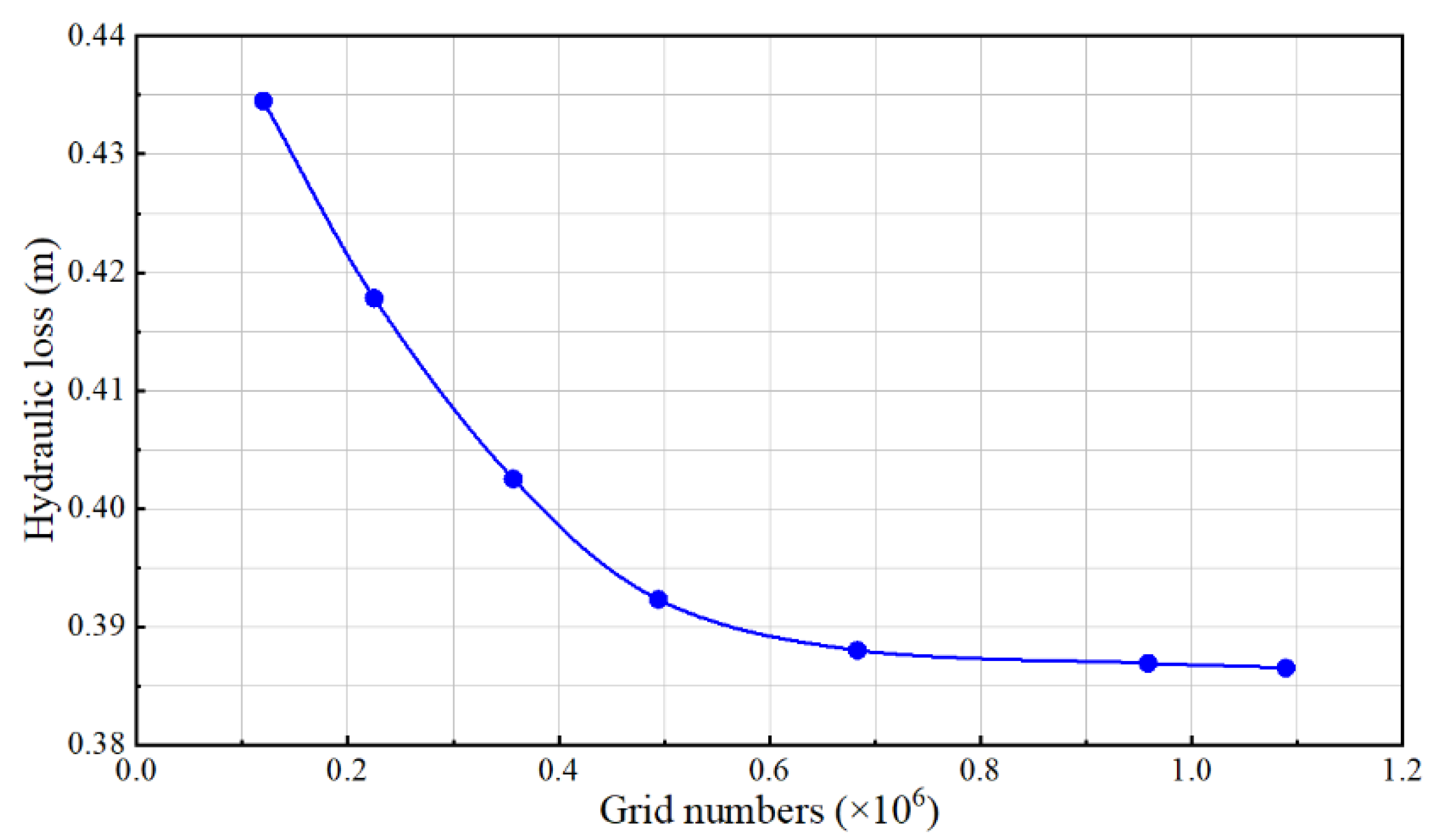
2.2.3. Mesh Generation and Calculation Setting

The mesh of flow field simulation domain of low hump outlet conduit was generated by soft of GAMBIT. The three-dimensional geometry of the low hump outlet conduit, whose inlet circular section transformed into the outlet rectangular section together with transition and diffusion, was comparatively complex. Thus, the unstructured mesh with more adaptability was applied for the outlet conduit. Mixed mesh and structural mesh were generated on the inlet straight pipe and the outlet sump. Two important measures of mesh quality were calculated in the Fluent solver: minimum orthogonal quality—0.26 is good; maximum aspect ratio—9.34 is acceptable because of the effect of boundary layer mesh. Mesh generation of the calculation domain is shown in Figure 4. In numerical calculation, convection-diffusion equations were handled by a first-order upwind difference scheme, pressure–velocity coupling equations were handled by the SIMPLEC algorithm, and convergence precision of calculation was set as 1 × 10⁻⁷.

Figure 5 is the variation law of hydraulic loss under different grid numbers. It could be seen that when the grid numbers are larger than 0.6 million, the relative error of hydraulic loss is less than 1%. The y+ value at inlet straight pipe, low hump outlet conduit, and outlet sump were 54~73, 42~57, and 82~96, respectively, which met the requirement of the RNG k-ε turbulence model with 30 < y+ < 300 [48]. Thus, for improving the precision and calculation efficiency of numerical simulation, the grid numbers of the calculation domain were finally adopted as 0.683 million. The grid distribution of computational domains is shown in

Table 2. Grid distribution of computational domains.

Domain	Inlet Straight Pipe	Low Hump Outlet Conduit	Outlet Sump
Grid number (×106)	0.025	0.502	0.156

.

2.3. Validation of Numerical Simulation Results

With the grid number of 0.683 million, five different turbulent models (the Spalart-Allmaras (S-A) turbulent model, the Standard k-ε turbulent model, the RNG k-ε turbulent model, the Realizable k-ε turbulent model, and the SST k-ω turbulent model) were used to carry out the numerical simulation. The comparison of hydraulic loss between numerical simulation (five different turbulent models) and model test is shown in Figure 6. It can be seen that with rotation speed increasing, the variation tendency of five turbulent models all firstly decreases and then increases, the hydraulic loss variation tendency of numerical simulation is consistent with that of the modified model test. When the rotation speed grows from 61 r/min to 300 r/min, the hydraulic loss of five numerical simulations is close to that of the modified model test; however, when rotation speed grows from 300 r/min to 390 r/min, the results difference between numerical simulation and the modified model test is gradually larger, significantly, in five different turbulent models, the RNG k-ε model results are closest to modified model test results. Thus, the RNG k-ε model is the most suitable one of the five different turbulent models and its results are consistent with the results of the modified model test.

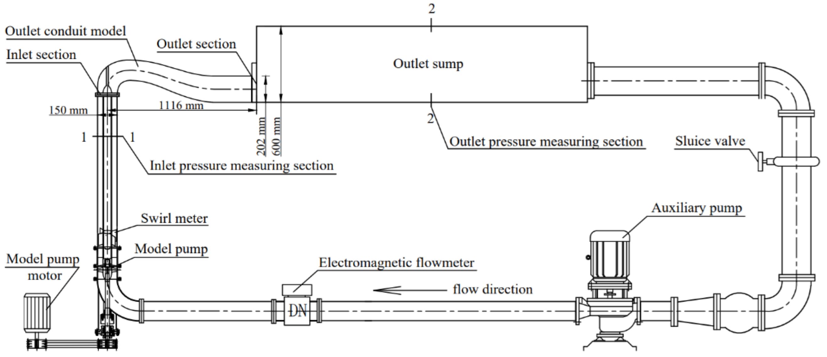
2.4. Device of Model Test

Figure 7 is the schematic diagram of model test device for the hydraulic performance of low hump outlet conduit. The model test device is a vertical circulation system and relevant apparatuses are labeled in it. The models of outlet conduit and outlet sump are made of transparent Perspex, which is convenient to observe and photograph the flow pattern of conduit. The flow pattern was shown by tracer red lines fixed on the inner wall of conduit instead of the PIV method [49,50] because of equipment limitation. The model pump, with impeller diameter 150 mm, is used to supply water. In addition, the other auxiliary pump, with an outlet diameter of 200 mm, is used to increase the ability of supplying water. The flow rate of test is adjusted by changing the rotation speed of auxiliary or opening of the sluice valve. The inlet of conduit is connected with an equal diameter straight round pipe and the outlet of conduit is connected with rectangular outlet sump. The inlet pressure measuring section is set to 200 mm before the inlet section of the outlet conduit. The outlet pressure measuring section is set a certain distance after the outlet section of the outlet conduit. The pressure measuring sections satisfy gradually varied flow conditions. At the closed section after the guide vane, the swirl meter, which has four pieces of straight blades, is set to measure the fluid rotation speed. The effect of the swirl meter blade numbers on the hydraulic loss of low hump outlet conduit has been studied in reference [1], the result indicates that the difference in conduit hydraulic loss between blade numbers of 4 and 0 is 1.86%. When the number of blades of the swirl meter is four, the swirl meter has little effect on the hydraulic loss of the outlet conduit. Thus, the swirl meter with four blades was selected. According to Bernoulli’s equation, the flow resistance of the outlet conduit was calculated using the following formula.

$$\mathrm{\Delta }h=\frac{1}{2g}({\overline{v}}_1^2-{\overline{v}}_2^2)+(H_1-H_2)-\mathrm{\Delta }{h}_{\mathrm{sp}}$$

(34)

where $\mathrm{\Delta }h$ is the hydraulic loss of outlet conduit; ${\overline{v}}_1^{}$ and ${\overline{v}}_2^{}$ are the mean velocities of cross-section 1-1 and cross-section 2-2, respectively; $H_1$ and $H_2$ are piezometer heads of cross-section 1-1 and cross-section 2-2, respectively; $\mathrm{\Delta }{h}_{\mathrm{sp}}$ is the hydraulic loss between cross-section 1-1 and the inlet cross-section of the outlet conduit.

The flow rate is measured by an electromagnetic flowmeter and the uncertainty of flow rate is ±0.5%. The static pressure is measured by piezometer tube and the uncertainty of static pressure is ±0.94%. The fluid rotation speed is measured by the swirl meter and the uncertainty of fluid rotation speed is ±1%. Thus, the total uncertainty of hydraulic loss of the low hump outlet conduit is ±2.72%, which meets the specification requirements of Rotodynamic pumps—Hydraulic performance acceptance tests—Grades 1, 2 and 3 [51]. The detailed introduction of the model test device and testing method were illustrated in reference [1,52].

Under diverse inlet water rotation speeds, the model test of hydraulic performance in the low hump outlet conduit was conducted to validate the results of numerical simulation. The picture of model test device is illustrated in Figure 8. To obtain different inlet water rotation speeds, five guide vanes with diverse blade shape, blade number and blade length were produced, and they were numbered from guide vane 1 to guide vane 5, respectively (Figure 9). Five guide vanes were, respectively, installed in the model test device, the fluid rotation speeds at different guide vanes outlet were measured and the corresponding hydraulic loss was calculated.

3. Results and Analysis

3.1. Results and Analysis of Numerical Calculation

Based on the above numerical simulation method and calculation settings, a three-dimensional numerical simulation of hydraulic performance in low hump outlet conduit was completed under the design discharge condition with different inlet water rotation speeds from 0 r/min to 400 r/min, respectively. Under the design discharge condition, the conduit hydraulic loss curve calculated under different inlet water rotation speeds is illustrated in Figure 10. As can be concluded from it: with the increase in inlet water rotation speed, the hydraulic loss of outlet conduit gradually decreases firstly, then it reaches minimum value when inlet water rotation speed is about 270 r/min; when the inlet water rotation speed is more than 270 r/min, the hydraulic loss increases, and the increasing rate is fast. The effect law of the inlet water rotation speed on the outlet conduit loss obtained in this study is similar to the results in Reference 5. However, when the rotation speed of the inlet water is small, the hydraulic loss of the outlet conduit is less affected by the rotation speed in this study, which is caused by the different hydraulic design parameters of the outlet conduit.

The swirl number is the ratio of tangential moment of momentum to axial moment of momentum. It is an important dimensionless parameter to represent swirl strength. The swirl number S of inlet cross-section of outlet conduit is as below:

$$S=\frac{{\displaystyle {\mathrm{\int }}_{R_1}^{R_2}{\displaystyle {\mathrm{\int }}_0^{2\mathsf{\pi }}{u}_{\mathrm{a}}{u}_{\mathrm{t}}{r}^2\mathrm{d}\theta \mathrm{d}r}}}{R{\displaystyle {\mathrm{\int }}_{R_1}^{R_2}{\displaystyle {\mathrm{\int }}_0^{2\mathsf{\pi }}{u}_{\mathrm{a}}^{2}r \mathrm{d}\theta \mathrm{d}r}}}$$

(35)

where $R_1$ is the inside radius of conduit inlet cross-section; $R_2$ is the outside radius of conduit inlet cross-section; $R$ is the equivalent radius of conduit inlet cross-section; $r$ is the distance to rotation axis; $\theta$ is the angle revolving around the rotation axis; $u_{\mathrm{a}}$ is the axial velocity; $u_{\mathrm{t}}$ is the tangential velocity.

The kinetic energy recovery coefficient is the key indicator to evaluate the hydraulic performance of outlet conduit. The higher the kinetic energy recovery coefficient is, the greater the recovery degree of outlet cross-section water kinetic energy is. The kinetic energy recovery coefficient of outlet conduit ${\eta }_{\omega }$ is as below:

$${\eta }_{\omega }=\frac{{\overline{v}}_{\mathrm{in}}^2/2g-{\overline{v}}_{\mathrm{out}}^2/2g-\mathrm{\Delta }{h}_{\mathrm{in}\text{-}\mathrm{out}}}{{\overline{v}}_{\mathrm{in}}^2/2g}$$

(36)

where ${\overline{v}}_{\mathrm{in}}$ is the mean inlet velocity of outlet conduit; ${\overline{v}}_{\mathrm{out}}$ is the mean outlet velocity of outlet conduit; $\mathrm{\Delta }{h}_{\mathrm{in}\text{-}\mathrm{out}}$ is hydraulic loss of outlet conduit.

The variation of the kinetic energy recovery coefficient of the outlet conduit in different swirl numbers is shown in Figure 11. With the increasing swirl number, the ${\eta }_{\omega }$ firstly slowly increases and then more quickly decreases. When the swirl number is 0.85, the ${\eta }_{\omega }$ is the max value. For further analysis, with the strengthening of swirl flow in outlet conduit, within the swirl number range of 0–0.85, the flow pattern is improved because of the rotation centrifugal force; thus, the hydraulic performance of outlet conduit is improved. Within the swirl number range of 0.85–1.24, the improving degree of the flow pattern of the outlet conduit decreases because of the higher swirl strength. In addition, the higher water velocity causes greater hydraulic loss than that improved by swirl flow; thus, the hydraulic performance of outlet conduit decreases.

In order to express the flow of water in the conduit, a section of the conduit shape closed to the wall of the conduit was selected to analyze the flow pattern under different inlet water rotation speeds. The schematic diagram of chosen section position (yellow) is shown in Figure 12. The flow patterns on the chosen section of low hump outlet conduit obtained by three-dimensional turbulent numerical simulation under conditions of design discharge and different inlet water rotation speeds are shown in Figure 13. Viewed in the direction of water flow, the outlet conduit is divided into left and right sides with the longitudinal centerline as the boundary. When the inlet water rotation speed is 0 r/min, the velocity distribution of the outlet conduit is of bilateral symmetry observed along the flow direction. At the inlet transition segment of the conduit, the flow makes a movement of turning 90 degrees and diffusion in the meanwhile, and the inside flow velocity of the conduit is greater than the outside. When the flow moves into the descent segment of the conduit after diversion, the main flow is closer to the upside of the conduit on account of flow motion inertia and circulation, and two large-scale symmetry vortexes are developed at the bottom of the conduit descent segment. The flow velocity is relatively uniform in the outlet straight segment of the conduit. With the increase in the inlet water rotation speed, the flow velocity in the conduit is also increased gradually, which leads flow velocity distribution in the conduit to be more asymmetrical. Because of the joint influence of flow motion inertia and rotation, the main flow is closer to the upside and left side of the conduit, and the vortex area gradually moved to the right side and downside of the conduit descent segment. Meanwhile, the vortex area becomes smaller and smaller. In addition, the origin of the vortex also gradually moved away from the descent segment inlet because of the stronger flow rotation. When the inlet water rotation speed comes to 400 r/min, the vortex in the conduit has been inexistent, the main flow in the descent segment of the conduit is closer to the bottom and left side, and the low-velocity area is moved to the right side and upside of the low hump outlet conduit.

Compared with the flow field of the low hump outlet conduit with different circulations studied in reference [53], the changing trend of the flow field of the two outlet flow conduits with the increase in the inlet water rotation speed is basically the same. Firstly, two symmetric vortex areas exist at the bottom of the conduit when the inlet water rotation speed is 0 r/min. Then, the vortex area becomes single and moves to the right bottom of conduit when the inlet water rotation speed is increased. Finally, the vortex area is eliminated when the inlet water rotation speed is high. However, due to the different hydraulic design parameters of the outlet conduit, the flow field distribution is different. The vortex area of outlet conduit in reference [53] is mainly located in the bottom of outlet straight segment, which is different from the location of the bottom of the descent segment in this research.

Based on the flow field of the low hump outlet conduit, further analysis of the variation tendency of hydraulic loss is as below: the hydraulic loss of the outlet conduit is determined by two aspects—flow velocity and flow pattern. Due to the growth of inlet water rotation speed, it will correspondingly add the flow velocity in conduit, which results in the increase in hydraulic loss, but in the meantime, it will narrow down the range of vortex area and improve the flow pattern, which results in the decrease in hydraulic loss.

When inlet water rotation speed grows, if the decrease in a hydraulic loss arising from improving flow pattern is higher than the increase in that arising from the adding flow velocity, the sum of the two losses will decline. Thus, while the inlet water rotation speed grows from 0 to 270 r/min, the loss will gradually decline. However, if the decrease in a hydraulic loss arising from improving flow pattern is lower than the increase in that arising from adding flow velocity, the sum of the two losses will rise. This is especially obvious under the larger inlet water rotation speed, because the vortex area in the conduit is already small, and the reduction in a hydraulic loss arising from the improving flow pattern is very limited. Thus, the loss of the low hump outlet conduit increases obviously when the inlet water rotation speed is higher than 270 r/min.

3.2. Results and Analysis of Model Test

Under design discharge conditions, the inlet water rotation speeds on the cross-sections of different guide vanes and corresponding hydraulic loss of outlet conduit are listed in

Table 3. Inlet water rotation speeds on the cross-sections of different guide vanes and corresponding hydraulic loss in outlet conduit under design flow.

Number of Guide Vane	Guide Vane 1	Guide Vane 2	Guide Vane 3	Guide Vane 4	Guide Vane 5
Inlet water rotation speed (r/min)	61	216	286	342	390
Hydraulic loss of conduit (m)	0.426	0.413	0.402	0.496	0.602
Modified hydraulic loss of conduit (m)	0.407	0.394	0.384	0.478	0.583

. According to model test results, the curve of hydraulic loss and inlet water rotation speed of the outlet conduit is shown in Figure 14. Significantly, the width and depth of outlet sump between numerical simulation and model test are different, which to some extent affects the exit loss of low hump outlet conduit; thus, the hydraulic loss of model test is revised by the computation method of exit loss in hydraulics [54]. Compared with the numerical simulation results, it could be seen that the conduit hydraulic loss of numerical simulation is close to that of the model test under lower inlet water rotation speed, but there is rather a difference between the two results under higher inlet water rotation speed. The variation tendency of conduit hydraulic loss of numerical simulation is in keeping with that of the model test. With the growing inlet water rotation speed, the hydraulic loss of the conduit firstly declines gradually and then rises remarkably.

The difference between numerical simulation results and modified model test results becomes larger after a rotation speed of 300 r/min. The main reasons are possible in two aspects—the turbulence model and discretization. With the increase in rotation speed, the turbulence flow is more complex in low hump outlet conduit and the RNG k-ε model is hard to make sure model constants; thus, the accurate results of numerical simulation are not obtained and the uncertainty of numerical simulation correspondingly increases [55]; The discretization scheme of numerical simulation is first order upwind scheme; it has better stability and convergence, but it can cause the accuracy reduction in simulation [56].

In the model test, the flow pattern in the low hump outlet conduit under five different guide vanes was observed and recorded, and the flow pattern was shown by tracer red lines fixed on the inner wall of conduit and particles immersed into water. The flow pattern pictures of outlet conduit under conditions of guide vanes 1, 3, and 5 are illustrated in this paper. Looking in the flow direction, the left view and right view of flow pattern in outlet conduit are illustrated by Figure 15a. For clearer observation of flow pattern variation in the conduit, partial enlarged drawings of descent segment of outlet conduit corresponding to the three different guide vanes are illustrated by Figure 15b–d. It is observed as follows: when guide vane 1 is installed, the flow rotation speed of outlet conduit and the inclination angle of tracer red lines are both smaller. Affected by the flow motion inertia, the large-scale vortex area (tracer red lines show reverse flow) is developed at the bottom of the descent segment in the conduit, and the vortex area is extended before the inlet of outlet straight segment. When the guide vane 3 is installed, the inlet water rotation speed of outlet conduit is increased, the main flow is closer to left side and the upside of the conduit, there is no vortex in the left area of the bottom of the descent segment, and the range is about half of the bottom width, meanwhile there is vortex in the right area of the bottom, and the vortex appeared in the lower part of the right side of the conduit. Compared with the guide vane 1, the range of vortex area becomes smaller. When guide vane 5 is installed, the inlet water rotation speed of outlet conduit is larger, the vortex area is inexistent at this time, the tracer red lines in the right side and upside of descent segment outlet of conduit swing in low speed and do not flow reversely, which indicates that there is the low flow velocity area.

Comparing the flow pattern between numerical simulation and model test, the locations of the main flow and vortex area are basically consistent. For main flow, with inlet water rotation speed of outlet conduit growing, the main flow in the model test is developed from the location closer to the upside of the conduit, then to the location closer to the upside and left side of the conduit, and finally to a location closer to the left side and downside of the conduit. The area in numerical simulation, which is displayed in the green area and smaller curvature streamlines, is the main flow area, it follows the same position change rule as the main flow in the model test. For the vortex area, with the inlet water rotation speed of the outlet conduit growing, the range of the vortex area becomes smaller from the location closer to the downside of the conduit, then to the location closer to the right side in the bottom of the conduit, and finally to a location closer to the downside in the right side of the conduit, the vortex area in the conduit will not exist when the flow rotation speed is large enough. The area in numerical simulation, which is displayed in the blue area and larger curvature streamlines, is the vortex area, and it follows the same position and range change rule as the vortex area in the model test.

4. Conclusions

(1)

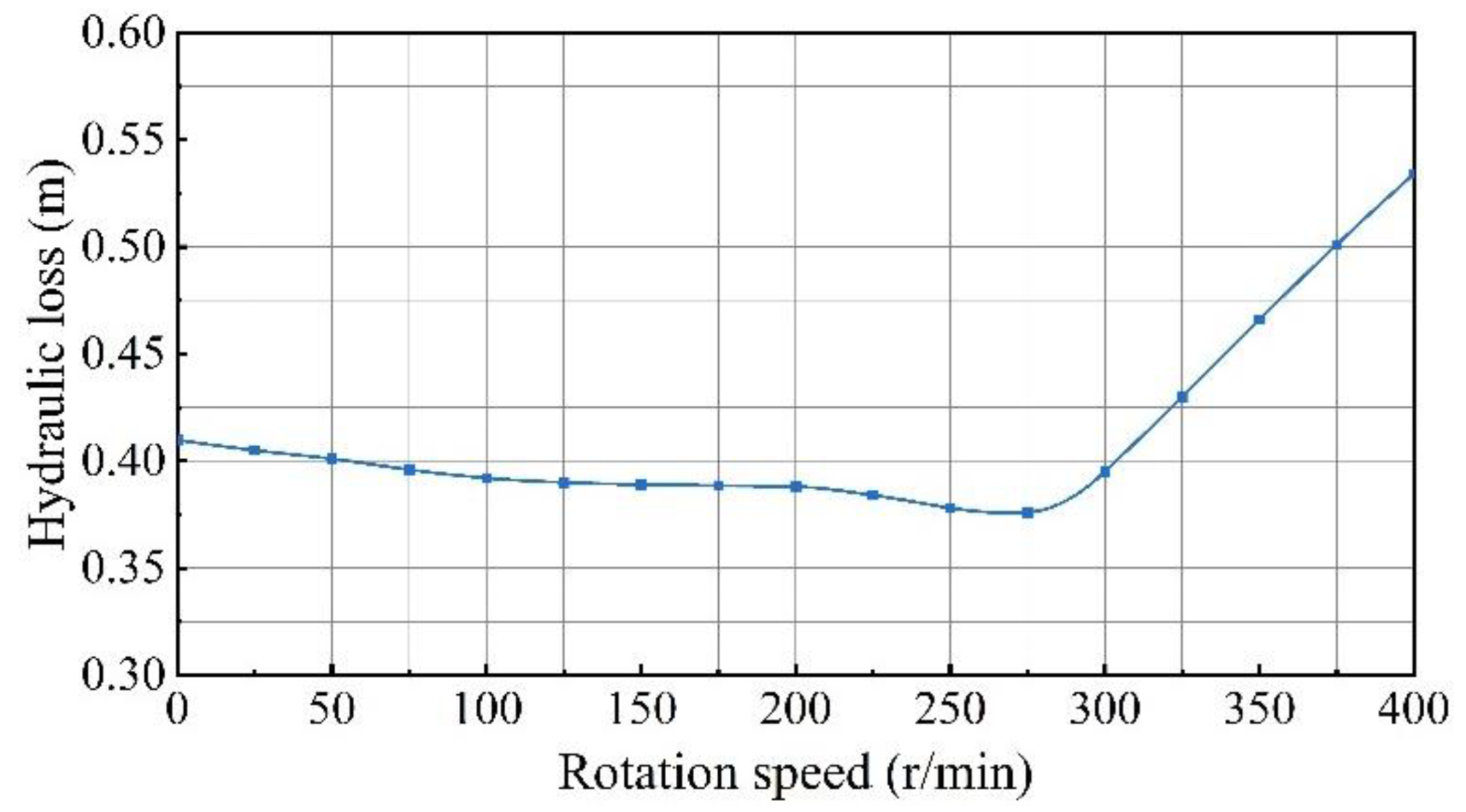
With the growing inlet water rotation speed in the low hump outlet conduit, the hydraulic loss of the conduit is firstly decreased gradually and then obviously increased. The reasons for the above results are as below: when the hydraulic loss is increased arising from growing flow rotation speed, the hydraulic loss is reduced arising from improving flow pattern. If the increased hydraulic loss is less than the reduced hydraulic loss, the hydraulic loss of the outlet conduit will decrease. On the contrary, the hydraulic loss will increase.

(2)

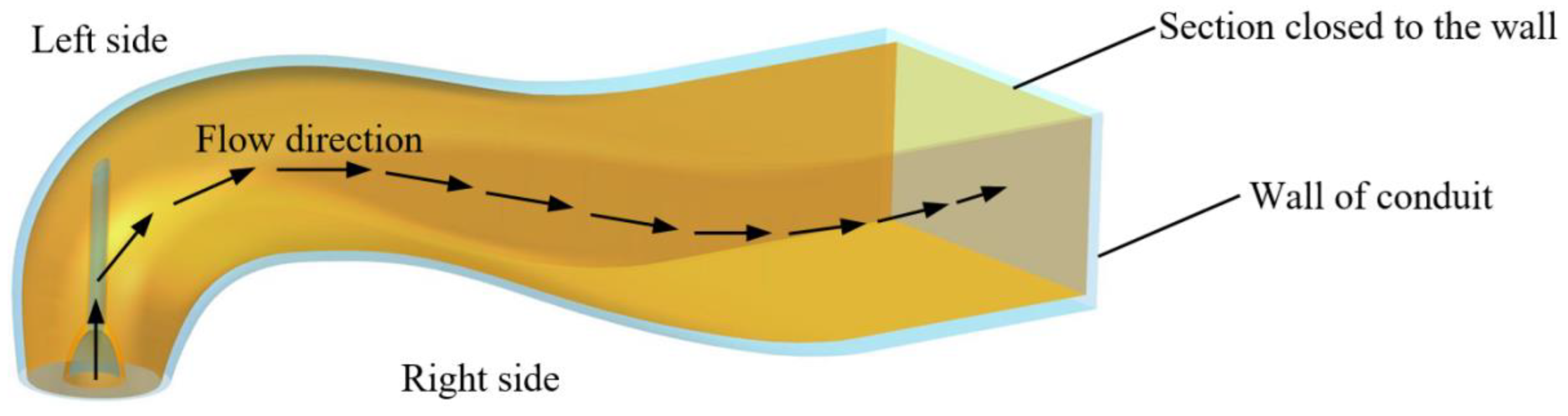
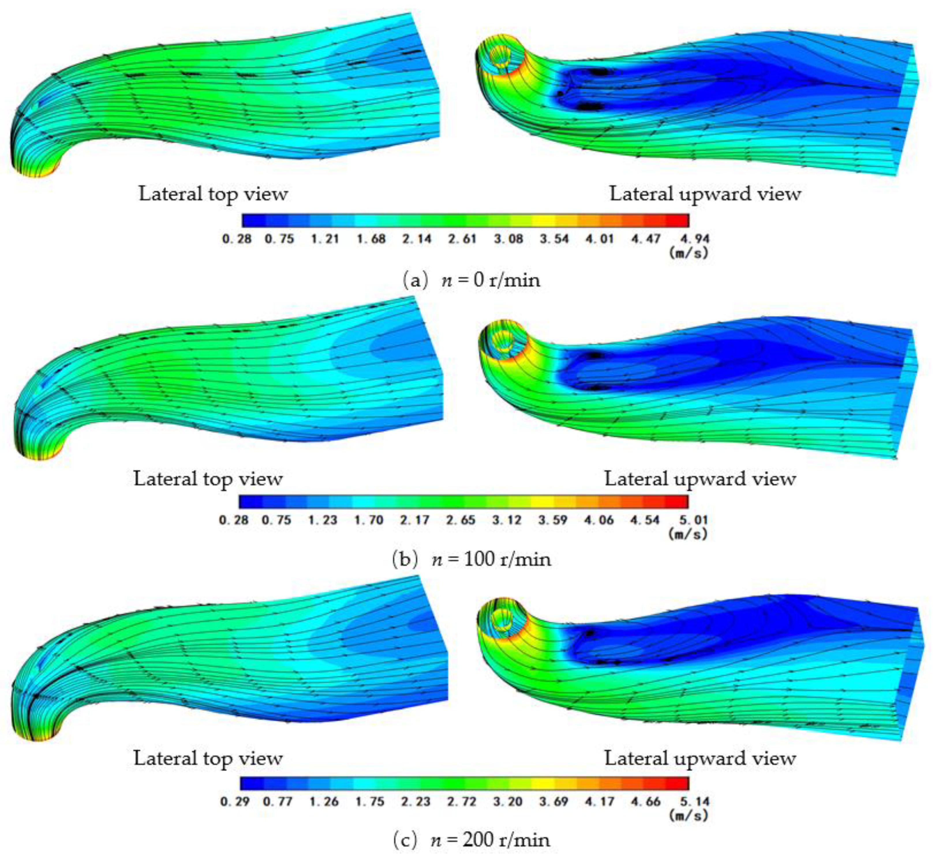
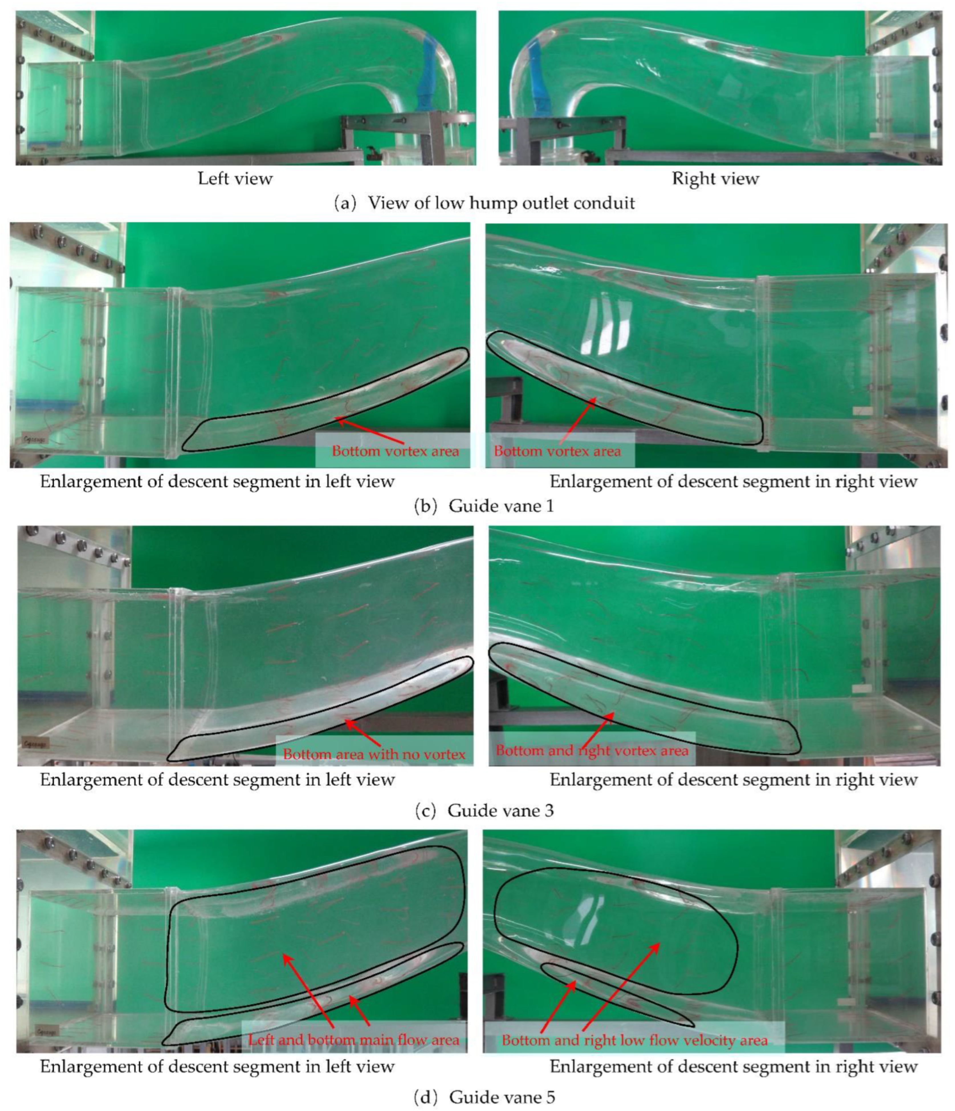
The flow pattern in the low hump outlet conduit is greatly influenced by the inlet water rotation speed, with the increase in the inlet water rotation speed, the location of the main flow area and vortex area will correspondingly change. When the inlet water rotation speed is 0 r/min, the bottom of the descending segment is covered with a symmetrical vortex. When the inlet water rotation speed is increased, the position of the vortex transfers to the lower right side of the conduit descends the segment, and the range of the vortex area is gradually decreased. While inlet water rotation speed grows to 400 r/min, the vortex field in the outlet conduit is inexistent.

(3)

The inlet water rotation speed of the low hump outlet conduit has a great impact on both hydraulic loss and flow pattern. The guide vane in the low head pump cannot completely eliminate the rotation speed of the water transmitted from the pump impeller. Therefore, the factor of the rotation speed of flow must be considered in the hydraulic optimum design of the outlet conduit, so that the hydraulic performance of the outlet conduit is optimized under the condition of a certain rotation speed.

(4)

The research results of this paper also have certain guiding functions to the hydraulic design of the guide vane in the low head pump, it is suggested that the guide vane is designed according to the flow rotation speed under which the hydraulic performance of the outlet conduit is optimal, so as to achieve the optimal matching between guide vane and outlet conduit in low head pump device. From the design of the guide vane in the low head pump, the numbers of blades in the guide vane of the existing low head pumps are mainly between five and seven [57], which is to ensure that the rotation speed of the water at the outlet conduit is not too large.

References

1. Lu, L.G. Optimized Hydraulic Design of Large-Scale High-Performance Pump Device with Low Head, 1st ed.; China Water & Power Press: Beijing, China, 2013. (In Chinese) [Google Scholar]
2. Lu, L.G.; Liu, J.; Liang, J.D.; Xu, L.; Huang, J.J.; Liu, R.H. Numerical simulation of 3D turbulent flow and hydraulic loss in outlet conduit of large pumping station. Drain. Irrig. Mach. 2008, 26, 51–54. (In Chinese) [Google Scholar]
3. Qiu, B.Y.; Lin, H.J.; Yuan, S.Q.; Huang, J.Y.; Feng, X.L. Optimum hydraulic design for discharge passage of large pump. Chin. J. Mech. Eng. 2006, 42, 47–51. (In Chinese) [Google Scholar] [CrossRef]
4. Karpenko, M.; Prentkovskis, O.; Sukevicius, S. Research on high-pressure hose with repairing fitting and influence on energy parameter of the hydraulic drive. Eksploat. Niezawodn.—Maint. Reliab. 2022, 24, 25–32. [Google Scholar] [CrossRef]
5. Ge, M.M.; Manikkam, P.; Ghossein, J.; Subramanian, R.K.; Coutier-Delgosha, O.; Zhang, G.J. Dynamic mode decomposition to classify cavitating flow regimes induced by thermodynamic effects. Energy 2022, 254, 124426. [Google Scholar] [CrossRef]
6. Ge, M.M.; Sun, C.Y.; Zhang, G.J.; Coutier-Delgosha, O.; Fan, D.X. Combined suppression effects on hydrodynamic cavitation performance in Venturi-type reactor for process intensification. Ultrason. Sonochemistry 2022, 86, 106035. [Google Scholar] [CrossRef]
7. Ge, M.M.; Zhang, G.J.; Petkovšek, M.; Long, K.P.; Coutier-Delgosha, O. Intensity and regimes changing of hydrodynamic cavitation considering temperature effects. J. Clean. Prod. 2022, 338, 130470. [Google Scholar] [CrossRef]
8. Ge, M.M.; Petkovšek, M.; Zhang, G.J.; Jacobs, D.; Coutier-Delgosha, O. Cavitation dynamics and thermodynamic effects at elevated temperatures in a small Venturi channel. Int. J. Heat Mass Transf. 2021, 170, 120970. [Google Scholar] [CrossRef]
9. McDonald, A.T.; Fox, R.W.; Van Dewoestine, R.V. Effect of swirling flow on pressure recovery in conical diffusers. AIAA J. 1971, 9, 2014–2018. [Google Scholar] [CrossRef]
10. Prakash, R.; Karthiek, N.; Ashwath, P.; Anand, H.; Adithya, G. Numerical study on a conical diffuser with inlet swirl. Appl. Mech. Mater. 2016, 852, 688–692. [Google Scholar]
11. Kaya, D. Experimental study on regaining the tangential velocity energy of axial flow pump. Energy Convers. Manag. 2003, 44, 1817–1829. [Google Scholar] [CrossRef]
12. Susan-Resiga, R.; Ciocan, G.D.; Anton, I.; Avellan, F. Analysis of the Swirling Flow Downstream a Francis Turbine Runner. J. Fluids Eng. 2005, 128, 177–189. [Google Scholar] [CrossRef]
13. Qiu, B.Y.; Huang, J.Y.; Yuan, S.Q.; Lin, H.J.; Feng, X.L.; Gao, C.H. Study on determination of water flow energy in section of outlet pipe of an axial flow pump. J. Hydroelectr. Eng. 2005, 24, 104–109. (In Chinese) [Google Scholar]
14. Liang, J.D.; Lu, L.G.; Xu, L.; Chen, W.; Wang, G. Influence of flow velocity circulation at guide vane outlet of axial-flow pump on hydraulic loss in outlet conduit. Trans. CSAE 2012, 28, 55–60. (In Chinese) [Google Scholar]
15. Qiu, B.Y.; Feng, X.L.; Yuan, S.Q. Analysis of flow deviation in two-channel discharge passage of a large pumping station. J. Hydroelectr. Eng. 2005, 24, 110–114. (In Chinese) [Google Scholar]
16. Qiu, B.Y.; Huang, J.Y.; Yuan, S.Q.; Lin, H.J.; Huang, J.Y. Test investigation on hydraulic losses in discharge passage of axial-flow pump. Chin. J. Mech. Eng. 2006, 42, 39–44. (In Chinese) [Google Scholar] [CrossRef]
17. Zhu, H.G. Numerical analysis on the internal flow of siphon discharge passages under off-design conditions. J. Hydroelectr. Eng. 2006, 25, 140–144. (In Chinese) [Google Scholar]
18. Zhu, H.G.; Yuan, S.Q. Performance effect of inlet flow field on siphon outlet conduit. Trans. Chin. Soc. Agric. Mach. 2006, 37, 193–196. (In Chinese) [Google Scholar]
19. Cai, J.L. Study on the Numerical Simulation of the Influence of the Outlet Circulation of Axial Flow Pump to the Hydraulic Loss of the Outlet Conduit. Master’s Thesis, Yangzhou University, Yangzhou, China, 2009. (In Chinese). [Google Scholar]
20. Fang, G.H.; Zhu, X.H.; Huang, X.F. Risk analysis of floodwater resources utilization along water diversion project: A case study of the Eastern Route of the South-to-North Water Diversion Project in China. Water Supply 2019, 19, 2464–2475. [Google Scholar] [CrossRef]
21. Lu, L.G.; Wu, K.P.; Leng, Y.; Chen, A.P. Hydraulic optimization design on straight outlet conduit of large-scale pumping station with low head. Trans. Chin. Soc. Agric. Mach. 2007, 38, 196–198. (In Chinese) [Google Scholar]
22. Wang, H.L.; Long, B.; Wang, C.; Han, C.; Li, L. Effects of the impeller blade with a slot structure on the centrifugal pump performance. Energies 2020, 13, 1628. [Google Scholar] [CrossRef]
23. Luo, H.; Zhou, P.; Shu, L.; Mou, J.; Zheng, H.; Jiang, C.; Wang, Y. Energy Performance Curves Prediction of Centrifugal Pumps Based on Constrained PSO-SVR Model. Energies 2022, 15, 3309. [Google Scholar] [CrossRef]
24. Zhou, P.J.; Dai, J.C.; Yan, C.S.; Zheng, S.H.; Ye, C.L.; Zhang, X. Effect of stall cells on pressure fluctuations characteristics in a centrifugal pump. Symmetry 2019, 11, 1116. [Google Scholar] [CrossRef] [Green Version]
25. Sun, Z.Z.; Wang, X.Y.; Shi, L.J.; Tang, F.P. Hydraulic performance and flow patterns of axial-flow pumps with axial stacking of different airfoil series. J. Drain. Irrig. Mach. Eng. 2022, 40, 217–222. (in Chinese). [Google Scholar]
26. Song, Y.; Gu, X.Y.; Liu, Y.Y.; Yin, J.L.; Wang, D.Z. Numerical simulation on pressure pulsation characteristic of nuclear coolant pump under different boundary conditions. J. Drain. Irrig. Mach. Eng. 2019, 37, 645–649. (In Chinese) [Google Scholar]
27. Xu, L.; Xia, B.; Shi, W.; Liu, J.; Yan, S.K.; Lu, L.G. Influence of middle pier lengths on hydraulic characteristic of outlet conduit in pump system with slanted extension shaft. Trans. Chin. Soc. Agric. Eng. 2020, 36, 74–81. (In Chinese) [Google Scholar]
28. Jiang, H.Y.; Yan, H.Q.; Xiao, Z.M.; Cheng, L.; Liu, H. Numerical simulation of hydraulic characteristics of three-side inlet of vertical shaft inlet channel of horizontal pumping station. J. Drain. Irrig. Mach. Eng. 2021, 39, 1008–1013. (In Chinese) [Google Scholar]
29. Tong, Z.M.; Yang, Z.Q.; Huang, Q.; Yao, Q. Numerical Modeling of the hydrodynamic performance of slanted axial-flow urban drainage pumps at shut-off condition. Energies 2022, 15, 1905. [Google Scholar] [CrossRef]
30. Lu, W.G.; Wang, D.W.; Shi, W.; Liu, J.; Xu, L. Comparison of hydraulic performance between submersible tubular pump device with motor front and rear arrangements. J. Drain. Irrig. Mach. Eng. 2020, 38, 325–331. (In Chinese) [Google Scholar]
31. Shi, W.; Cheng, L. Analysis of effect of blades angle on hydraulic performance for pumping system of water diversion pumping station. J. Drain. Irrig. Mach. Eng. 2020, 38, 372–377. (In Chinese) [Google Scholar]
32. Teuber, K.; Broecker, T.; Bayón, A.; Nützmann, G.; Hinkelmann, R. CFD-modelling of free surface flows in closed conduits. Prog. Comput. Fluid Dyn. 2019, 6, 368–380. [Google Scholar] [CrossRef]
33. Simão, M.; Pérez-Sánchez, M.; Carravetta, A.; López-Jiménez, P.; Ramos, H.M. Velocities in a Centrifugal PAT Operation: Experiments and CFD Analyses. Fluids 2018, 3, 3. [Google Scholar] [CrossRef] [Green Version]
34. Rezvaya, K.; Krupa, E.; Shudryk, A.; Drankovskiy, V. Solving the hydrodynamical tasks using CFD programs. In Proceedings of the International Conference on Intelligent Energy and Power Systems, Kharkiv, Ukraine, 10–14 September 2018; pp. 205–209. [Google Scholar]
35. Gunjo, D.G.; Mahanta, P.; Robi, P.S. CFD and experimental investigation of flat plate solar water heating system under steady-state condition. Renew. Energy 2017, 106, 24–36. [Google Scholar] [CrossRef]
36. Seyedashraf, O.; Akhtari, A.A. Three-dimensional CFD study of free-surface flow in a sharply curved 30° open-channel bend. J. Eng. Sci. Technol. Rev. 2017, 10, 85–89. [Google Scholar] [CrossRef]
37. Ziaei, A.N.; Nikou, N.S.; Beyhaghi, A.; Beyhaghi, F.; Khodashenas, S.R. Flow simulation over a triangular labyrinth side weir in a rectangular channel. Prog. Comput. Fluid Dyn. 2019, 19, 22–34. [Google Scholar] [CrossRef]
38. Zhou, P.J.; Yan, C.S.; Shu, L.F.; Wang, H.; Mou, J.G. Effects of particle concentration on the dynamics of a single-channel sewage pump under low-flow-rate condition. FDMP-Fluid Dyn. Mater. Process. 2021, 17, 871–886. [Google Scholar] [CrossRef]
39. Adhikari, R.; Wood, D. Computational Analysis of a Double-Nozzle Crossflow Hydroturbine. Energies 2018, 11, 3380. [Google Scholar] [CrossRef] [Green Version]
40. Zhang, D.; Wang, H.; Liu, J.; Wang, C.; Ge, J.; Zhu, Y.; Chen, X.; Hu, B. Flow characteristics of oblique submerged impinging jet at various impinging heights. J. Mar. Sci. Eng. 2022, 10, 399. [Google Scholar] [CrossRef]
41. Hu, B.; Wang, H.; Liu, J.; Zhu, Y.; Wang, C.; Ge, J.; Zhang, Y. A numerical study of a submerged water jet impinging on a stationary wall. J. Mar. Sci. Eng. 2022, 10, 228. [Google Scholar] [CrossRef]
42. Yakhot, V.; Orszag, S.A. Renormalization group analysis of turbulence. I. basic theory. J. Sci. Comput. 1986, 1, 3–51. [Google Scholar] [CrossRef] [Green Version]
43. Wang, F.J. Computational Fluid Dynamics Analysis—Principle and Application, 1st ed.; Tsinghua University Press: Beijing, China, 2004. (In Chinese) [Google Scholar]
44. Ibrahim, K.A.; Hamed, M.H.; El-Askary, W.A.; El-Behery, S.M. Swirling gas–solid flow through pneumatic conveying drye. Powder Technol. 2013, 235, 500–515. [Google Scholar] [CrossRef]
45. Shi, L.J.; Yuan, Y.; Jiao, H.F.; Tang, F.P.; Chen, L.; Yang, F.; Jin, Y.; Zhu, J. Numerical investigation and experiment on pressure pulsation characteristics in a full tubular pump. Renew. Energy 2021, 163, 987–1000. [Google Scholar] [CrossRef]
46. Stachnik, M.; Jakubowski, M. Multiphase model of flow and separation phases in a whirlpool: Advanced simulation and phenomena visualization approach. J. Food Eng. 2020, 274, 109846. [Google Scholar] [CrossRef]
47. Rodi, W. Turbulence Models and Their Application in Hydraulics: A State of the-Art Review, 3rd ed.; Balkema: Rotterdam, The Netherlands, 2017. [Google Scholar]
48. Ariff, M.; Salim, S.M.; Cheah, S.C. Wall y+ approach for dealing with turbulent flow over a surface mounted cube: Part 1—low Reynolds number. In Proceedings of the Seventh International Conference on CFD in the Minerals and Process Industries, Melbourne, VIC, Australia, 9–11 December 2009; pp. 1–6. [Google Scholar]
49. Sterczyńska, M.; Jakubowski, M. Research on Particles’ Velocity Distribution in a Whirlpool Separator Using the PIV Method of Measurement. Int. J. Food Eng. 2017, 13, 20160316. [Google Scholar] [CrossRef]
50. Sterczynsk, M.; Stachnik, M.; Poreda, A.; Piepiorka-Stepuk, J.; Zdaniewicz, M.; Jakubowsk, M. The improvement of flow conditions in a whirlpool with a modified bottom: An experimental study based on particle image velocimetry (PIV). J. Food Eng. 2021, 289, 110164. [Google Scholar] [CrossRef]
51. ISO 9906-2012; Rotodynamic Pumps—Hydraulic Performance Acceptance Tests—Grades 1, 2 and 3. ISO: Geneva, Switzerland, 2012. (In Chinese)
52. Lu, L.G.; Wu, K.P.; Leng, Y.; Zhu, J. Measurement for hydraulic loss of outlet conduit of pumping station. Drain. Irrig. Mach. 2005, 23, 23–26. (In Chinese) [Google Scholar]
53. Lu, W.G.; Dong, L.; Wang, Z.F.; Lu, L.L. Cross influence of discharge and circulation on head loss of conduit of pump system with low head. Appl. Math. Mech. 2012, 33, 1533–1544. [Google Scholar] [CrossRef]
54. Wu, C.G. Hydraulics, 5th ed.; Higher Education Press: Beijing, China, 2016. (In Chinese) [Google Scholar]
55. Zhang, X.L.; Xiao, H.; Gomez, T.; Coutier-Delgosha, O. Evaluation of ensemble methods for quantifying uncertainties in steady-state CFD applications with small ensemble sizes. Comput. Fluids 2020, 203, 104530. [Google Scholar] [CrossRef] [Green Version]
56. Ge, M.M.; Zhang, X.L.; Brookshire, K.; Coutier-Delgosha, O. Parametric and V&V study in a fundamental CFD process: Revisiting the lid-driven cavity flow. Aircr. Eng. Aerosp. Technol. 2022, 94, 515–530. [Google Scholar]
57. Liu, N.; Wang, Y.S.; Zhang, G. Pump Model Test of South-to-North Water Diversion in Same Bench, 1st ed.; China Water & Power Press: Beijing, China, 2006. (In Chinese) [Google Scholar]
Figure 1. Single-line diagram of model low hump outlet conduit (unit: mm).
Energies 15 05371 g001
Figure 2. Three-dimensional model diagram of low hump outlet conduit.
Energies 15 05371 g002
Figure 3. Flowchart of research methods.
Energies 15 05371 g003
Figure 4. Calculation domain of flow field simulation and mesh generation.
Energies 15 05371 g004
Figure 5. Variation law of hydraulic loss under different grid numbers.
Energies 15 05371 g005
Figure 6. Comparison of hydraulic loss between numerical simulation (five different turbulent models) and model test.
Energies 15 05371 g006
Figure 7. Schematic diagram of model test vertical circulation system of low hump outlet conduit.
Energies 15 05371 g007
Figure 8. Model test device of low hump outlet conduit.
Energies 15 05371 g008
Figure 9. Series of guide vanes.
Energies 15 05371 g009
Figure 10. Numerical results of hydraulic loss in outlet conduit under different inlet water rotation speeds.
Energies 15 05371 g010
Figure 11. Variation of kinetic energy recovery coefficient of outlet conduit in different swirl numbers.
Energies 15 05371 g011
Figure 12. Schematic diagram of section position.
Energies 15 05371 g012
Figure 13. Flow field of low hump outlet conduit under different inlet water rotation speeds.
Energies 15 05371 g013aEnergies 15 05371 g013b
Figure 14. Model test results of hydraulic loss of outlet conduit under different inlet water rotation speeds.
Energies 15 05371 g014
Figure 15. Pictures of flow pattern in outlet conduit under different guide vanes.
Energies 15 05371 g015