Article

Low-Cost I–V Tracer for PV Fault Diagnosis Using Single-Diode Model Parameters and I–V Curve Characteristics

1
GeePs, CentraleSupélec, CNRS, Université Paris-Saclay/Sorbonne Université, 3-11 Rue Joliot Curie, 91192 Gif Sur Yvette, France
2
CNRS, CentraleSupélec, Université Paris-Saclay, L2S, 3 Rue Joliot Curie, 91192 Gif Sur Yvette, France
3
IUT Cachan, Université Paris-Saclay, 9 Avenue de la Division Leclerc, 94230 Cachan, France
*
Author to whom correspondence should be addressed.
Energies 2022, 15(15), 5350; https://doi.org/10.3390/en15155350
Submission received: 21 June 2022 / Revised: 19 July 2022 / Accepted: 20 July 2022 / Published: 23 July 2022

Abstract

:
The continuous health monitoring of PV modules is mandatory to maintain their high efficiency and minimize power losses due to faults or failures. In this work, a low-cost embedded tracer is developed to measure the I–V curve of a PV module in less than 0.2 s. The data are used to extract the five parameters of the single-diode model and its main characteristics (open-circuit voltage, short-circuit current, and maximum power). Experimental data are used to validate the analytical model and evaluate the two fault diagnosis methods, using as fault features the parameters of the single-diode model or the main characteristics of the I–V curve. The results, based on field data under different temperatures and irradiances, show that the degradation of series and shunt resistances could be detected more accurately with the main characteristics rather than with the parameters. However, the estimated parameters could still be used to monitor the long-term degradation effects.

1. Introduction

According to the International Energy Agency (IEA), renewable energy will contribute 80% of the world’s electricity generation by 2030. This growth will be mainly driven by solar photovoltaic energy [1]. At the end of 2020, the total installed photovoltaic (PV) capacity reached 760 GW , with an increase of 139 GW since 2019 [2].
However, due to PV modules being located outdoors, they can be exposed to harsh conditions (e.g., humidity, snow, sand, dirt, and moisture). They may also be damaged during transportation or installation [3,4]. The faulty PV panels will exhibit lower performances [5]. It is reported that annual energy losses due to various faults could reach up to 18.9% during the first year of operation [6]. In other studies, the energy losses range between 22 and 27% during fifteen months of operation for fifteen PV power plants in Spain and Italy due to inefficiency (shading and soiling effects, PV module degradation, temperature impact, etc.) [7].
In order to limit the drop in performance and improve the reliability of the PV panels, it is necessary to set up condition-based maintenance based on continuous monitoring. Fault detection and diagnosis (FDD) are the heart of health monitoring. There are several FDD approaches reported in the literature [8,9,10]. They can broadly be classified as either visual inspection or automatic analysis. Visual inspection is suitable for small-scale PV systems, but may require an expert to analyze the information. Automatic analysis methods are based on the analysis of fault features [11] obtained from measured or estimated information. The most usual information captured from PV systems is the coordinates and the power at the maximum power point (MPP) or the I–V curves obtained with I–V tracers.
The fault diagnosis method, based on the power at the MPP, analyzes the power actually produced using the maximum power point tracking (MPPT) algorithm [12,13]. In [14], three fault indicators are calculated from the comparison between the predicted and the measured current, voltage, and power at the MPP. However, they are sensitive to a limited number of faults.
The I–V curve can be partially or fully used for fault diagnosis. In the case of partial usage, only several points are analyzed to make a decision. For example, open-circuit voltage (Voc), short-circuit current (Isc), and the power at the MPP (Pmpp) [15] can be used. The disadvantages of this approach are the limited number of diagnosable faults and its high sensitivity to environmental conditions.
In the case of full usage (as in [16]), the full I–V curve is used as a fault feature for PV fault diagnosis under eight different conditions (healthy and seven faults), with variable temperatures and irradiances. Six machine learning techniques (artificial neural network, support vector machine, decision tree, random forest, k-nearest neighbors, and naive Bayesian classifier) were evaluated. The main issues are related to the number of sampling points and the computational burden necessary to handle the data processing. The full I–V curve can also be used to extract the PV model parameters (Iph, I0, Rs, Rsh and n) considered as fault features. In [17], this approach was used with the double-diode model. Various types of partial shading (PS) and degradation are diagnosed using threshold analysis. The effectiveness of this method depends strongly upon the accuracy of the model used.
However, the I–V curve is a widely discussed topic [8] because the I–V curve contains several pieces of information about the health of the PV module. However, to obtain this curve, it is necessary to have a tracer and to interrupt production during the measurement. It is, therefore, a challenge to offer an I–V tracer at a reasonable cost that limits production losses.
In our study, two FDD methodologies are evaluated. The first one uses the parameters of the electrical equivalent circuit as fault features. It is based on the single-diode model (SDM). The second one uses the PV module current and voltage vectors Ipv, Vpv and the extracted characteristics Pmpp, Isc, and Voc as fault features. The first contribution of this paper is the proposal of a low-cost embedded I–V tracer with a logarithmic distribution of the points (LDP) on the I–V curve to reduce the measurement time. The second contribution is the experimental validation of the analytical equations used to calculate the parameters of the SDM. Finally, the paper proposes an evaluation of series resistance, shunt resistance, and partial shading fault detection, using either SDM parameters or I–V curves characteristic points as fault features under a wide variety of environmental conditions.
This paper is organized as follows: in Section 2, the experimental test bench is presented. Section 3 describes the four steps to identify and validate the single diode PV model. Section 4 presents the hybrid PV model of the PV model. Section 5 introduces the methodologies of PV panel fault detection and diagnosis and presents the diagnosis results. Conclusions are drawn in the last section.

2. Experimental Test Bench

The schematic diagram of the experimental test is shown in Figure 1.
The central part of the experimental setup was the I–V tracer developed during this research project. This I–V tracer was calibrated and validated via a high-efficiency E4360A modular solar array simulator (MSAS) keysight, with an accuracy of 1.33% in the healthy case. Furthermore, several measurement devices were included:
  • A TC 74 temperature sensor glued on the backside of the PV module was used to measure the temperature ( T p v ) . The operating range of the sensor was −40 °C to 125 °C, with ±3 °C accuracy from +25 °C to +85 °C.
  • The plane of array irradiance ( G p o a ) was measured using a reference cell (model Si-RS485TC-T-MB monocrystalline silicon irradiance sensors) with a tilt angle of 25 ° , identical to the PV panel’s support structure.
The data (I–V curve, G p o a , and T p v ) were collected and stored. Several other parameters were computed and could be displayed: I m p p , V m p p , P m p p , I s c , and V o c . It also allowed the I–V and P–V curves of the module to be displayed under actual environmental conditions. In addition, the emulations of different faults were developed to study the degradation of PV modules, by connecting additional resistances in series and parallel, as shown in Figure 2. The parameters of the PV module under test (installed in 2010) are displayed in Table 1.

2.1. Low-Cost I–V Tracer

Many research works have proposed different I–V tracers for PV cell/module/string and array with a high resolution and fast computation [18,19,20]. The number of points is a compromise between the duration of the measurement, which should be as short as possible to minimize the loss of power due to the interruption, and the required accuracy for post-processing. In healthy conditions, the I–V curve can be split into three parts:
  • The constant current zone, in which few points could be sufficient;
  • The almost constant voltage zone, for which a low resolution could be acceptable;
  • The area around the maximum power point, where a high resolution is necessary.
In the literature, there are several proposals on how to distribute the points on the I–V curve. In the following, the logarithmic distribution of points (LDP) was used, as displayed in Figure 3. N b P t V is the number of points distributed from 0 to V m p p , and N b P t I is the number of points distributed from I m p p to 0. In the following, they were set to 12 and 15, respectively. These values depended on the equivalent resistance of the I–V tracer.
The voltage and current of the PV module were measured with a resistive voltage divider and a shunt resistor. The measurement for one point was obtained from the average over 100 periods to reduce the negative effects of switching, followed by a relaxation time. Therefore, the acquisition time for one point was 7 ms, and the measurement time for the 26 points (there was a common measurement point for both areas) of the full I–V curve was approximately 182 ms. The process is described in Figure 4.
The developed I–V tracer circuit is shown in Figure 5. The components of the instrument were sized according to the PV modules studied: 10 A, 30 V, and 100 W, for current, voltage, and power, respectively. It consisted of voltage and current sensors, relays, a variable resistor, and a microcontroller, whose functions were the following:
  • To control the relays that allowed for the disconnecting of the PV module from the string during the I–V curve measurement;
  • To generate the duty cycle of the PWM that allowed for having a variable load resistance. The switching frequency was 50 kHz;
  • To send the data to the computer through a serial link (see Figure 2).
Finally, the cost of the prototype was 35 €/unit. Of course, the final cost would be greatly reduced for mass production. Eventually, the I–V tracer is expected to be installed in a box on the back of the PV module. A comparison with market I–V tracers is shown in Table 2.

2.2. Preprocessing of I–V Curves

After the acquisition on a sunny day of 205 I–V curves from 9:30 a.m. to 4:20 p.m., it was observed that some of them exhibited an abnormal shape due to the activation of a bypass diode (see the red circled area in Figure 6). A visual inspection revealed that an air conditioning aluminum tube was responsible for the inhomogeneous irradiation received by the PV panel (Figure 7). To avoid any misinterpretation or wrong parameter identification, the abnormal curves were withdrawn using an interpolation technique. The remaining 128 curves are displayed in Figure 8. In the following, all of the measured curves were preprocessed before being used.

3. Identification of the Single-Diode Model Parameters

3.1. Five Parameters of the Single-Diode Model

The Single-Diode Model (SDM) displayed in Figure 9, with its five parameters, is an equivalent electrical circuit widely adopted for silicon PV cells [27,28]. It includes the photocurrent, the diode saturation current, and ideality factor, the series resistance, and the shunt resistance.
A PV module is composed of Ns cells in series, as shown in Figure 10. The corresponding I–V relationship is written as:
I p v = I p h I 0 [ e x p ( q ( V p v N s + I p v R s ) n K T K ) 1 ] ( V p v N s + I p v R s R s h )
where I p v refers to the PV current, I p h defines the photo-generated current, I 0 denotes the diode saturation current, q represents the electron’s charge ( q = 1.602 × 10 19 C ), V p v is the voltage, R s and R s h are the series and shunt resistances, n is the diode ideality factor, and K is Boltzmann’s constant ( K = 1.3806 × 10 23   J / K ). T K refers to the PV module temperature in kelvin.
The five parameters strongly depend on the irradiance and the temperature. Several research works have proposed analytical models for each of them. In the following, only the most accurate models for our installation were retained and presented.

3.1.1. Photocurrent (Iph)

The photocurrent ( I p h ) can be determined by using the following equation [29,30]:
I p h = I s c _ r e f [ 1 + k i _ r e f ( T p v T S T C ) ] G p o a G S T C
where T p v and T S T C represent the PV module’s actual and STC temperatures, respectively, in °C, and G p o a and G S T C are the actual and STC irradiances, respectively. The coefficients I s c _ r e f and k i _ r e f will be recalculated according to the actual environmental conditions. Their initial values were obtained from the datasheet (Table 1).

3.1.2. Diode Saturation Current (I0)

The diode saturation current ( I 0 ) can be obtained from Equation (3) [31,32]:
I 0 = I s c _ r e f [ 1 + k i _ r e f ( T p v T S T C ) ] e x p ( q V o c _ r e f [ 1 + K v _ r e f ( T p v T S T C ) ] n K N s T K ) 1
The coefficients V o c _ r e f and k v _ r e f will be recalculated according to the actual environmental conditions. Their initial values were obtained from the datasheet (Table 1).

3.1.3. Series Resistance (Rs)

The series resistance ( R s ) was representative of the I–V curve in the almost constant voltage area. The following relation was adopted [33,34]:
R s = R s _ r e f [ T K T n × ( 1 β r e f l n ( G p o a G S T C ) ) ]
The coefficients R s _ r e f and β r e f will be recalculated according to the actual environmental conditions. The initial value of R s _ r e f was estimated from a one-shot I–V curve measurement, while the initial value of β r e f was taken from the literature. T n was the temperature at STC in kelvin.

3.1.4. Shunt Resistance (Rsh)

The shunt resistance ( R s h ) was representative of the I–V curve in the constant current area. The authors in [35,36,37] have proposed an analytical model of R s h as described below:
R s h = R s h _ r e f × G S T C G p o a
The coefficient R s h _ r e f will be recalculated according to the actual environmental conditions. Its initial value was estimated from a one-shot I–V curve.

3.1.5. Diode Ideality Factor (n)

The diode ideality factor (n) depends linearly only on the temperature, and it can be expressed as below [38,39]:
n ( T p v ) = n r e f × T K T n
where n r e f   is the diode ideality factor. Its initial value was set to 1 as usual.

3.2. Identification of the SDM Parameters

The identification method of the vector of parameters θ = [ I p h ,   R s ,   R s h ,   I 0 ,   n ] was based on the Levenberg–Marquardt (LM) optimization algorithm. The LM algorithm [40,41] provides a numerical solution to the problem of minimizing the quadratic error:
M i n θ ( ( I V ) m e a s ( I V ) e s ) 2
where ( I V ) e s represents the relation between the voltage and the current of the PV module. It was calculated from Equation (1). Furthermore. ( I V ) m e a s was the measured I–V curve.

3.3. Model Validation

PV cell manufacturers provided the characteristics and parameters at STC (cf. Table 1), which were insufficient to determine the overall PV performance. Indeed, an accurate model of the PV system under any environmental conditions was required, because PV cells operate under variable weather conditions.
In the following, a 4-step methodology, described in Figure 11, was developed to extract the parameters of the SDM. The first two were devoted to the training, while the last two were for the validation.
  • Step 1: for the training data ( T p v ,   G p o a ) t r a i n i n g , measure the I–V curves, and identify θ ^ ( I V ) = [ I p h ,   R s ,   R s h ,   I 0 ,   n ] ;
  • Step 2: Identify the eight reference values
    δ r e f = [ R s h _ r e f ,   R s _ r e f ,   β r e f ,   V o c _ r e f ,   k v _ r e f ,   k i _ r e f ,   I s c _ r e f ,   n r e f ] of the analytical models. Consider the cross-effect between G p o a and T p v ;
  • Step 3: Estimate θ ^ a n a l y = [ I ^ p v ,   R ^ s ,   R ^ s h ,   I ^ 0 ,   n ^ ] with the analytical models, using the reference values and the validation data ( T p v ,   G p o a ) v a l i d a t i o n ;
  • Step 4: Analyze for each of the (I–V) curves (M curves are measured) the mean absolute percentage error ( M A P E θ ) between θ ^ ( I V ) and θ ^ a n a l y to validate the analytical model.
M A P E θ = 100 M i = 1 M | θ ^ ( I V ) ( i ) θ ^ a n a l y ( i ) θ ^ ( I V ) ( i ) |

3.3.1. Training Step

For the training data ( G p o a , T p v ) t r a i n i n g , 488 I–V curves were measured for G p o a 600   W / m 2 , as shown in Table 3.

Analytical Model of the Photocurrent (Iph)

According to Equation (2), the photocurrent depends on the reference coefficients k i _ r e f ,   and   I s c _ r e f . Their initial values were determined from the datasheet. The photocurrent depends not only on the irradiance but also on the temperature. To avoid the cross-effect between G p o a and T p v , the extraction of the PV model parameters was evaluated with constant G p o a or T p v . Under different irradiances for T p v = 56 °C corresponding to 73 (I–V) curves, the reference parameters were estimated. The results are shown in Figure 12.
The evolution of I p h with G p o a is shown in Figure 12. The analytical model converged toward the measured values. The M A P E I p h was 6.01%.
Once the reference coefficient temperature ( k i _ r e f ) was estimated for constant T p v , (see in Table 4), its value was set in Equation (2). Then I s c _ r e f was estimated for constant G p o a . We assumed that 750 W/m2Gpoa ≤ 780 W/m2, which corresponded to 103 (I–V) curves. The results are displayed in Table 5. The initial value for I s c _ r e f was the optimal value determined in the previous section (Table 4).
The evolution of I p h as the function of T p v is shown in Figure 13. It can be observed the temperature T p v has a slight influence on I p h . The M A P E I p h was equal to 1.49%.

Analytical Model of the Diode Saturation Current (I0)

As can be noticed in Equation (3), I 0 only depended on the temperature and the reference values V o c _ r e f , k v _ r e f , I s c _ r e f , and k i _ r e f . The last two were determined in the previous section.
Figure 14 and Table 6 show the results. I 0 slightly increased with T p v . The M A P E I 0 , was equal to 7.34%.

Analytical Model of the Series Resistance (Rs)

According to Equation (4), the analytical model of R s depended on the irradiance and the temperature, with two reference values of R s _ r e f and β r e f . Firstly, the reference values were determined for constant T p v = 56 °C. The results are presented in Table 7 and Figure 15.
The value of β r e f was set in Equation (4) to analyze the influence of the temperature.
The results of the extraction for constant irradiation are shown in Figure 16 and Table 8, respectively.
We can observe that R s increased linearly with T p v . The M A P E R s is 0.92%.

Analytical Model of the Shunt Resistance (Rsh)

In this section, the analytical model in Equation (5) was investigated to estimate the reference value R s h _ r e f . The evolution of R s h as a function of G p o a is shown in Figure 17. The result demonstrated that shunt resistance ( R s h ) was inversely proportional to the irradiance ( G p o a ).
The coefficient R s h _ r e f that is the reference value in Equation (5) was extracted, and is displayed in Table 9. The optimized value was 49.85 Ω, and the M A P E R s h was 7.4%.

Analytical Model of the Diode Ideality Factor (n)

The analytical model of the diode ideality factor n in Equation (6) depended on the temperature and the reference value n r e f . The estimation result is displayed in Table 10. Figure 18 shows that n was almost constantly over the temperature variation range.

3.3.2. Validation Step

Table 11 summarizes the eight reference values extracted from the training data of the 488 I–V curves. These values were used to estimate with the analytical models the five parameters of the PV model θ ^ , with the environmental validation data ( G p o a , T p v ) v a l i d a t i o n distinct from those used for training. The information of the validation data are displayed in Table 12.
The uncertainties in the estimation errors of the different parameters are displayed in Figure 19. The results showed significant dispersion for all the parameters, mainly because of the variable environmental conditions. Despite the scattered uncertainties in the estimation errors of the five parameters, the analytical models remain valid. In reality, only four parameters could be determined from measurements. There was, therefore, a degree of freedom to obtain the correct I–V characteristic for several parameter combinations. Finally, the vector of parameters estimated from the analytical models can be used to evaluate the performance of the PV array under different irradiances and temperatures.

4. Hybrid Model of the PV Module

A hybrid model was developed to evaluate the performance of the PV array. It was comprised of the analytical model determined in the previous section combined with the numerical PV model in MATLAB/Simulink®. To evaluate its accuracy, the data obtained from the hybrid model were compared to the ones measured with the I–V tracer.
The methodology is described in Figure 20. The information on the testing data are displayed in Table 13.
The vector X 1 is defined as [ I p v ] or [ V p v ] , and the scalar X 2 is defined as P m p p , or   I s c , or   V o c .
The following errors were computed: the mean absolute percentage error ( M A P E ( X 1 ) ) and the absolute relative error ( A R E ( X 2 ) ):
M A P E ( X 1 ) = 100 M i = 1 M | X 1 m e a s ( i ) X 1 s i m ( i ) X 1 m e a s ( i ) |
A R E ( X 2 ) = 100 | X 2 m e a s X 2 s i m | X 2 m e a s
where M is the number of I–V curves.
The histograms plotted in Figure 21 show that the errors between the experimental and the simulated values were lower than 3%. Therefore, we can conclude that the hybrid model is suitable for health monitoring because it is accurate and robust to environmental conditions.

5. Fault Detection and Diagnosis

5.1. Methodology

PV systems under operation are prone to several faults. Due to natural aging or severe environmental conditions (e.g., a decrease in contact adhesion and the corrosive action of water vapor), the series resistance increases, while the shunt resistance decreases. In the following, the degradation of series and shunt resistances will be considered through two scenarios:
  • Fault 1: R s degradation
  • Fault 2: R s h degradation
Two FDD methodologies are proposed. The first one, denoted “M1”, displayed in Figure 22a, uses the parameters of the equivalent electric circuit as fault features. The second one, “M2”, shown in Figure 22b, uses the characteristics I p v , V p v , P m p p , I s c , and   V o c extracted from the I–V curves as fault features.

5.2. Rs Degradation

The series resistance ( R s ) represents the resistance of the cell and the connection resistance between the cells. Its degradation is due to aging or aggressive environmental conditions. Δ R s 1 , Δ R s 2 , and Δ R s 3 are three additional resistances added in series with the PV panel to emulate three fault levels (f1, f2, f3), corresponding to an increase of 28%, 42%, and 50%, respectively. Table 14 displays the fault scenarios, the environmental conditions, and the number of I–V curves measured with the I–V tracer. Temperature T p v and irradiance G p o a are also provided.

5.2.1. FDD with Method M1

As described in Figure 22a, the FDD method M1 uses the vector of parameters as fault features. In the following, R s ( I V ) stands for the series resistance extracted from the measured I–V curve, while R s ( a n a l y ) is the series resistance estimated from the analytical model. The lower script ‘f’ stands for faulty, and ‘h’ for healthy.
From the histograms displayed in Figure 23, we can draw the following conclusions:
  • In the healthy case, despite the variations in the environmental conditions (irradiance and temperature), the series resistance R s h [ 0.737 ,   0.788 ]   Ω is almost constant;
  • In faulty conditions, the series resistances are significantly different from the healthy case;
  • A threshold set at ε R s , t h = 3 ( σ R s ( a n a l y ) , h ) m a x 0.04   Ω will allow for the detection of each fault.
The histograms of the residuals are plotted in Figure 24. The fault can be detected because for each case, ϵ > R s t h . The severity levels can also be estimated with a good accuracy, as shown in Table 15.
From the results shown in Figure 25, it is interesting to notice that the degradation of the series resistance has almost no effect on the other parameters of the SDM.

5.2.2. FDD with Method M2

As displayed in Figure 22b, the method M2 was based on the analysis of the residuals between the main characteristics extracted from measured I–V curves and those obtained from the hybrid model. The results are displayed in Figure 26. The red points are singular points in the distribution.
The relative variations of the mean values (compared to the healthy case) for the five characteristics are displayed in Table 16 (the bold values correspond to the best results). We can deduce that the maximum power point (Figure 26c) is the most sensitive to the series resistance degradation. The values of the voltage (Figure 26b) are also more affected than the PV module’s current values (Figure 26a). The open-circuit voltage (Figure 26d) and the short-circuit current (Figure 26e) are barely affected. These results are consistent, as the series resistance mainly affects the voltage source region of the I–V curve.

5.3. Rsh Degradation

The parallel resistance represents all of the paths crossed by the leakage current, either in parallel with the cell or at the cell’s border. Its degradation results from damage in the crystal or impurities in or near the junction.

5.3.1. FDD with Method M1

For the experiment, R s h _ a d d 1 , R s h _ a d d 2 , and R s h _ a d d 3 were the resistances added in parallel with the PV panel to emulate three fault levels for R s h degradation. Table 17 summarizes the data acquisition for the faulty cases.
From the histograms displayed in Figure 27, we can draw the following conclusions:
  • In the healthy case, due to variations in the environmental conditions (irradiance and temperature), the shunt resistance ( R s h [ 54 , 71 ]   Ω ) varies slightly (Figure 27a);
  • In faulty conditions, the shunt resistances are significantly different from the healthy case (Figure 27a);
  • A threshold set at R s h t h = 3 ( σ R s h e s , h ) m a x 4.5   Ω will allow for the detection of each fault;
  • the mean values of the residuals (Figure 27b) are consistent with the calculated variations Δ R s h = R s h , m e a n , h R s h , f [Ω] displayed in Table 18.
The fault effect on the other parameters plotted in Figure 28 shows that there is no significant variation.

5.3.2. FDD with Method M2

The influences of the R s h degradation on the other characteristics are shown in Figure 29. The boxplots are used to depict the comparisons between data obtained from being measured and from being simulated. The red points are singular points in the distribution. The following is a summary of the findings:
The relative variations of the mean values (compared to the healthy case) for the five characteristics are presented in Table 19 (bold values are the best results). From these results, it can be deduced that the maximum power point (Figure 29c) is the most sensitive to the degradation of the shunt resistance.
The values of the PV module’s current (Figure 29a) are also more significantly affected than the voltage values (Figure 29b). The open-circuit voltage (Figure 29d) and short circuit current (Figure 29e) are only slightly affected. These results are consistent with the fact that the shunt resistance mainly affects the current-source region of the I–V curve.

6. Conclusions

In this paper, two methodologies (denoted M1 and M2) of fault detection and diagnosis (FDD) for PV systems were developed and evaluated. M1 uses the five parameters ( I p h ,   R s ,   R s h ,   I 0   a n d   n ) of the single-diode model as fault features, while M2 uses the five characteristics ( I p v ,   V p v ,   P m p p ,   V o c ,   a n d   I s c ) of the I–V curves as fault signatures. M1 is based on analytical models of the parameters, and M2 exploits a hybrid model, which is a combination of the analytical models and a numerical model of the PV cells.
A low-cost embedded I–V tracer was developed and implemented to measure the I–V curves. It is based on a variable resistance obtained with a switching device. The results show that an accurate I–V curve with 26 points can be measured in less than 200 ms.
First, the analytical models are validated with experimental data. Despite the scattered uncertainties in the estimation errors of the five parameters, the analytical models remain valid. In reality, only four parameters can be determined from the measurements. There is, therefore, a degree of freedom to obtain the correct I–V characteristic for several combinations of the parameters. The hybrid model is validated with a relative error lower than 3%. Residuals are calculated between the fault features extracted from experimental measurements and the simulated models. Two fault cases are studied: series resistance ( R s ) degradation and shunt resistance ( R s h ) degradation.
In the case of R s and R s h degradation, the results with the method M1 show that the defect could be detected accurately, and its level estimated. The results also show that the other parameters are not affected. The results with the method M2 in both fault cases show that the maximum power point is the most sensitive fault feature. The performances of the methods are summarized in Table 20.

Author Contributions

Conceptualization, V.K., A.M.-D., C.D., J.-Y.L. and D.D.; methodology, V.K., A.M.-D., C.D., J.-Y.L. and D.D.; formal analysis, V.K., A.M.-D., C.D., J.-Y.L. and D.D.; investigation, V.K., A.M.-D., C.D., J.-Y.L. and D.D.; writing—original draft preparation, V.K. and D.D.; supervision, A.M.-D., C.D., J.-Y.L. and D.D.; writing—review and editing, V.K., A.M.-D., C.D., J.-Y.L. and D.D.; All authors have read and agreed to the published version of the manuscript.

Funding

This research received no external funding.

Institutional Review Board Statement

Not applicable.

Informed Consent Statement

Not applicable.

Data Availability Statement

Data is available on reasonable request to the authors.

Conflicts of Interest

The authors declare no conflict of interest.

References

  1. World Energy Outlook 2020. Technical Report of International Energy Agency. 2020. Available online: https://iea.blob.core.windows.net/assets/a72d8abf-de08-4385-8711-b8a062d6124a/WEO2020.pdf (accessed on 12 May 2022).
  2. REN21. Renewables 2021 Global Status Report. Technical Report of the Renewable Energy Policy Network for the 21st Century, Paris. 2021. Available online: https://www.ren21.net/wp-content/uploads/2019/05/GSR2021_Full_Report.pdf (accessed on 12 May 2022).
  3. Alam, M.K.; Khan, F.; Johnson, J.; Flicker, J. A Comprehensive Review of Catastrophic Faults in PV Arrays: Types, Detection, and Mitigation Techniques. IEEE J. Photovolt. 2015, 5, 982–997. [Google Scholar] [CrossRef]
  4. di Lorenzo, G.; Araneo, R.; Mitolo, M.; Niccolai, A.; Grimaccia, F. Review of O&M Practices in PV Plants: Failures, Solutions, Remote Control, and Monitoring Tools. IEEE J. Photovolt. 2020, 10, 914–926. [Google Scholar] [CrossRef]
  5. Maghami, M.R.; Hizam, H.; Gomes, C.; Radzi, M.A.; Rezadad, M.I.; Hajighorbani, S. Power loss due to soiling on solar panel: A review. Renew. Sustain. Energy Rev. 2016, 59, 1307–1316. [Google Scholar] [CrossRef] [Green Version]
  6. Firth, S.K.; Lomas, K.J.; Rees, S.J. A simple model of PV system performance and its use in fault detection. Sol. Energy 2010, 84, 624–635. [Google Scholar] [CrossRef] [Green Version]
  7. Lillo-Bravo, I.; González-Martínez, P.; Larrañeta, M.; Guasumba-Codena, J. Impact of energy losses due to failures on photovoltaic plant energy balance. Energies 2018, 11, 363. [Google Scholar] [CrossRef] [Green Version]
  8. Mellit, A.; Tina, G.M.; Kalogirou, S.A. Fault detection and diagnosis methods for photovoltaic systems: A review. Renew. Sustain. Energy Rev. 2018, 91, 1–17. [Google Scholar] [CrossRef]
  9. Köntges, M.; Kurtz, S.; Packard, C.; Janh, U.; Berger, K.A.; Gato, K.; Friesen, T.; Liu, H.; Iseghem, M.V. Review of Failures of Photovoltaic Modules. Report IEA-PVPS T13-01:2014. 2014. Available online: https://iea-pvps.org/wp-content/uploads/2020/01/IEA-PVPS_T13-01_2014_Review_of_Failures_of_Photovoltaic_Modules_Final.pdf (accessed on 12 May 2022).
  10. Madeti, S.R.; Singh, S.N. A comprehensive study on different types of faults and detection techniques for solar photovoltaic system. Sol. Energy 2017, 158, 161–185. [Google Scholar] [CrossRef]
  11. Delpha, C.; Diallo, D. Kullback-Leibler divergence for incipient fault diagnosis. In Signal Processing for Fault Detection and Diagnosis in Electric Machines and Systems; Institution of Engineering and Technology: Stevenage, UK, 2021; pp. 85–118. ISBN 987-1-78561-957-1. [Google Scholar]
  12. Mohanty, S.; Subudhi, B.; Ray, P.K. A Grey Wolf-Assisted Perturb & Observe MPPT Algorithm for a PV System. IEEE Trans. Energy Convers. 2017, 32, 340–347. [Google Scholar] [CrossRef]
  13. Yang, B.; Yu, T.; Zhang, X.; Li, H.; Shu, H.; Sang, Y.; Jiang, L. Dynamic leader based collective intelligence for maximum power point tracking of PV systems affected by partial shading condition. Energy Convers. Manag. 2018, 179, 286–303. [Google Scholar] [CrossRef]
  14. Chaibi, Y.; Malvoni, M.; Chouder, A.; Boussetta, M.; Salhi, M. Simple and efficient approach to detect and diagnose electrical faults and partial shading in photovoltaic systems. Energy Convers. Manag. 2019, 196, 330–343. [Google Scholar] [CrossRef]
  15. Huang, J.M.; Wai, R.J.; Gao, W. Newly-designed fault diagnostic method for solar photovoltaic generation system based on IV-Curve measurement. IEEE Access 2019, 7, 70919–70932. [Google Scholar] [CrossRef]
  16. Li, B.; Delpha, C.; Migan-Dubois, A.; Diallo, D. Fault diagnosis of photovoltaic panels using full I–V characteristics and machine learning techniques. Energy Convers. Manag. 2021, 248, 114785. [Google Scholar] [CrossRef]
  17. Ali, M.H.; Rabhi, A.; el Hajjaji, A.; Tina, G.M. Real Time Fault Detection in Photovoltaic Systems. Energy Procedia 2017, 111, 914–923. [Google Scholar] [CrossRef]
  18. Zhu, Y.; Xiao, W. A comprehensive review of topologies for photovoltaic I–V curve tracer. Sol. Energy 2020, 196, 346–357. [Google Scholar] [CrossRef]
  19. Campos, R.E.; Sako, E.Y.; Dos Reis, M.V.G.; Villalva, M.G. A review of the main methods to trace the I–V characteristic curve of PV sources. In Proceedings of the 2018 13th IEEE nternational Conference on Industry Application, Sao Paulo, Brazil, 12–14 November 2019; pp. 24–30. [Google Scholar] [CrossRef]
  20. Duran, E.; Piliougine, M.; Sidrach-De-Cardona, M.; Galan, J.; Andujar, J.M. Different methods to obtain the I–V curve of PV modules: A review. In Proceedings of the 33rd IEEE Photovoltaic Specialist Conference, San Diego, CA, USA, 11–16 May 2008. [Google Scholar]
  21. FTV2000 IV Tracer. Available online: https://chauvin-arnoux.fi/wp-content/uploads/2014/07/FTV200_GB.pdf (accessed on 12 May 2022).
  22. I–V 500W Tracer. Available online: https://www.ht-instruments.com/en/products/i-v525w/download/brochure/ (accessed on 12 May 2022).
  23. Electronic Load Model 63600 Series. Available online: https://www.chromaate.com/downloads/catalogue/Power/63600-EN.pdf (accessed on 12 May 2022).
  24. MP-11 I–V Checker|EKO Instruments. Available online: https://eko-eu.com/products/solar-energy/iv-measurements/mp-11-i-v-checker (accessed on 12 May 2022).
  25. Huawei. Smart I–V Curve Diagnosis. 2020. Available online: https://solar.huawei.com/en-GB/download?p=%252F-%252Fmedia%252FSolar%252Fattachment%252Fpdf%252Feu%252Fdatasheet%252FIV-Curve.pdf (accessed on 12 May 2022).
  26. Solmetric PV Analyzer I-V Curve Tracer User’s Guide with SolSensor TM 200 PVA-600 + with SolSensor TM. Available online: www.solmetric.com (accessed on 12 May 2022).
  27. Mehta, H.K.; Warke, H.; Kukadiya, K.; Panchal, A.K. Accurate Expressions for Single-Diode-Model Solar Cell Parameterization. IEEE J. Photovolt. 2019, 9, 803–810. [Google Scholar] [CrossRef]
  28. Şentürk, A. New method for computing single diode model parameters of photovoltaic modules. Renew. Energy 2018, 128, 30–36. [Google Scholar] [CrossRef]
  29. di Piazza, M.C.; Luna, M.; Petrone, G.; Spagnuolo, G. Parameter translation for single-diode PV models based on explicit identification. In Proceedings of the IEEE InternationalConference on Environment and Electrical Engineering and IEEE Industrial and Commercial Power System Europe (EEEIC/I&CPS Europe), Milan, Italy, 6–9 June 2017. [Google Scholar] [CrossRef]
  30. Xing, W.; Zhou, J.; Feng, Z. Effects of mounting geometries on photovoltaic module performance using CFD and single diode model. Sol. Energy 2014, 103, 541–549. [Google Scholar] [CrossRef]
  31. Dave, M.K. Modeling of PV arrays based on datasheet. In Proceedings of the 1st IEEE International Conference on Power Electronics, Intelligent Control and Energy System (ICPEICES), Dehi, India, 4–6 July 2017; pp. 1–4. [Google Scholar] [CrossRef]
  32. Villalva, M.G.; Gazoli, J.R.; Filho, E.R. Comprehensive approach to modeling and simulation of photovoltaic arrays. IEEE Trans. Power Electron. 2009, 24, 1198–1208. [Google Scholar] [CrossRef]
  33. Bai, J.; Liu, S.; Hao, Y.; Zhang, Z.; Jiang, M.; Zhang, Y. Development of a new compound method to extract the five parameters of PV modules. Energy Convers. Manag. 2014, 79, 294–303. [Google Scholar] [CrossRef]
  34. Ibrahim, H.; Anani, N. Variations of PV module parameters with irradiance and temperature. Energy Procedia 2017, 134, 276–285. [Google Scholar] [CrossRef]
  35. Brano, V.L.; Orioli, A.; Ciulla, G.; di Gangi, A. An improved five-parameter model for photovoltaic modules. Sol. Energy Mater. Sol. Cells 2010, 94, 1358–1370. [Google Scholar] [CrossRef]
  36. de Soto, W.; Klein, S.A.; Beckman, W.A. Improvement and validation of a model for photovoltaic array performance. Sol. Energy 2006, 80, 78–88. [Google Scholar] [CrossRef]
  37. Ruschel, C.S.; Gasparin, F.P.; Costa, E.R.; Krenzinger, A. Assessment of PV modules shunt resistance dependence on solar irradiance. Sol. Energy 2016, 133, 35–43. [Google Scholar] [CrossRef]
  38. Chouder, A.; Silvestre, S.; Sadaoui, N.; Rahmani, L. Modeling and simulation of a grid connected PV system based on the evaluation of main PV module parameters. Simul. Model. Pract. Theory 2012, 20, 46–58. [Google Scholar] [CrossRef]
  39. Jordehi, A.R. Parameter estimation of solar photovoltaic (PV) cells: A review. Renew. Sustain. Energy Rev. 2016, 61, 354–371. [Google Scholar] [CrossRef]
  40. Tossa, A.K.; Soro, Y.M.; Azoumah, Y.; Yamegueu, D. A new approach to estimate the performance and energy productivity of photovoltaic modules in real operating conditions. Sol. Energy 2014, 110, 543–560. [Google Scholar] [CrossRef]
  41. Dkhichi, F.; Oukarfi, B.; Fakkar, A.; Belbounaguia, N. Parameter identification of solar cell model using Levenberg–Marquardt algorithm combined with simulated annealing. Sol. Energy 2014, 110, 781–788. [Google Scholar] [CrossRef]
Figure 1. Schema diagram of the test bed.
Energies 15 05350 g001
Figure 2. Pictures of the experimental test bench.
Energies 15 05350 g002
Figure 3. Logarithmic distribution of points on the I–V curve.
Energies 15 05350 g003
Figure 4. Acquisition time.
Energies 15 05350 g004
Figure 5. Main circuit of the I–V tracer.
Energies 15 05350 g005
Figure 6. The 205 I–V characteristics in the healthy case measured on 2 September 2019.
Energies 15 05350 g006
Figure 7. Over-illumination effect (circled in red) on the PV panel.
Energies 15 05350 g007
Figure 8. 128 I–V curves after withdrawing the abnormal ones.
Energies 15 05350 g008
Figure 9. Single-diode model PV cell equivalent circuit.
Energies 15 05350 g009
Figure 10. Single-diode model for a PV module with Ns cells in series.
Energies 15 05350 g010
Figure 11. Methodology for parameters extraction.
Energies 15 05350 g011
Figure 12. Evolution of the photocurrent with Gpoa for Tpv = 56 °C.
Energies 15 05350 g012
Figure 13. Evolution of the photocurrent (Iph) with Tpv for 750 W/m2Gpoa ≤ 780 W/m2.
Energies 15 05350 g013
Figure 14. Evolution of the diode saturation current (I0).
Energies 15 05350 g014
Figure 15. Evolution of Rs for constant Tpv.
Energies 15 05350 g015
Figure 16. Evolution of Rs for constant Gpoa.
Energies 15 05350 g016
Figure 17. Evolution of Rsh for constant Tpv.
Energies 15 05350 g017
Figure 18. Evolution of the diode ideality factor (n).
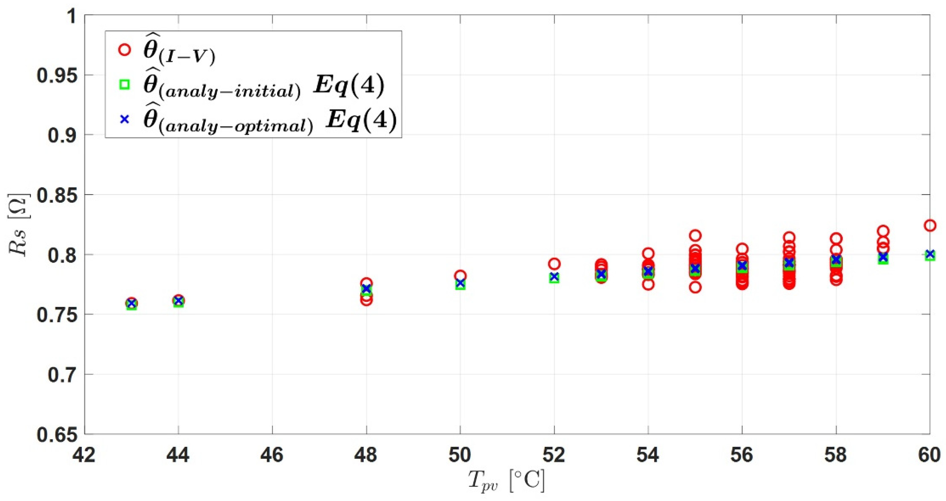
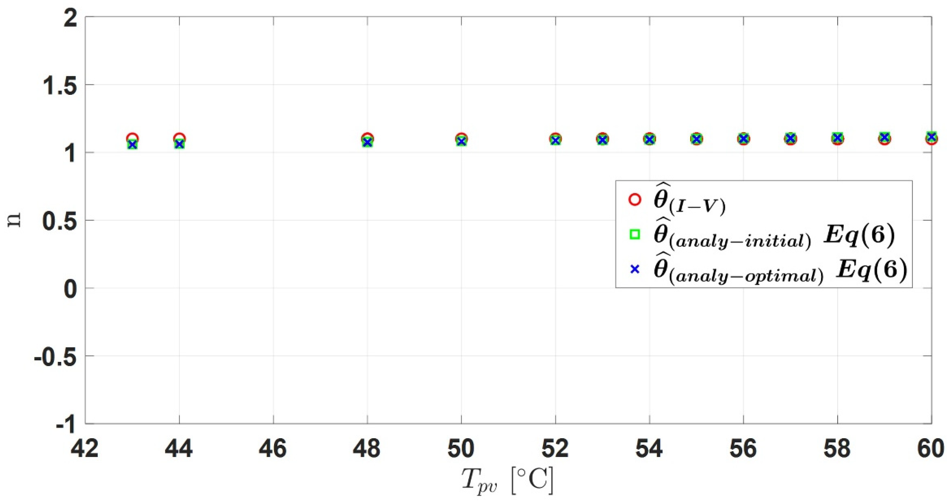
Energies 15 05350 g018
Figure 19. Estimation of the SDM parameters.
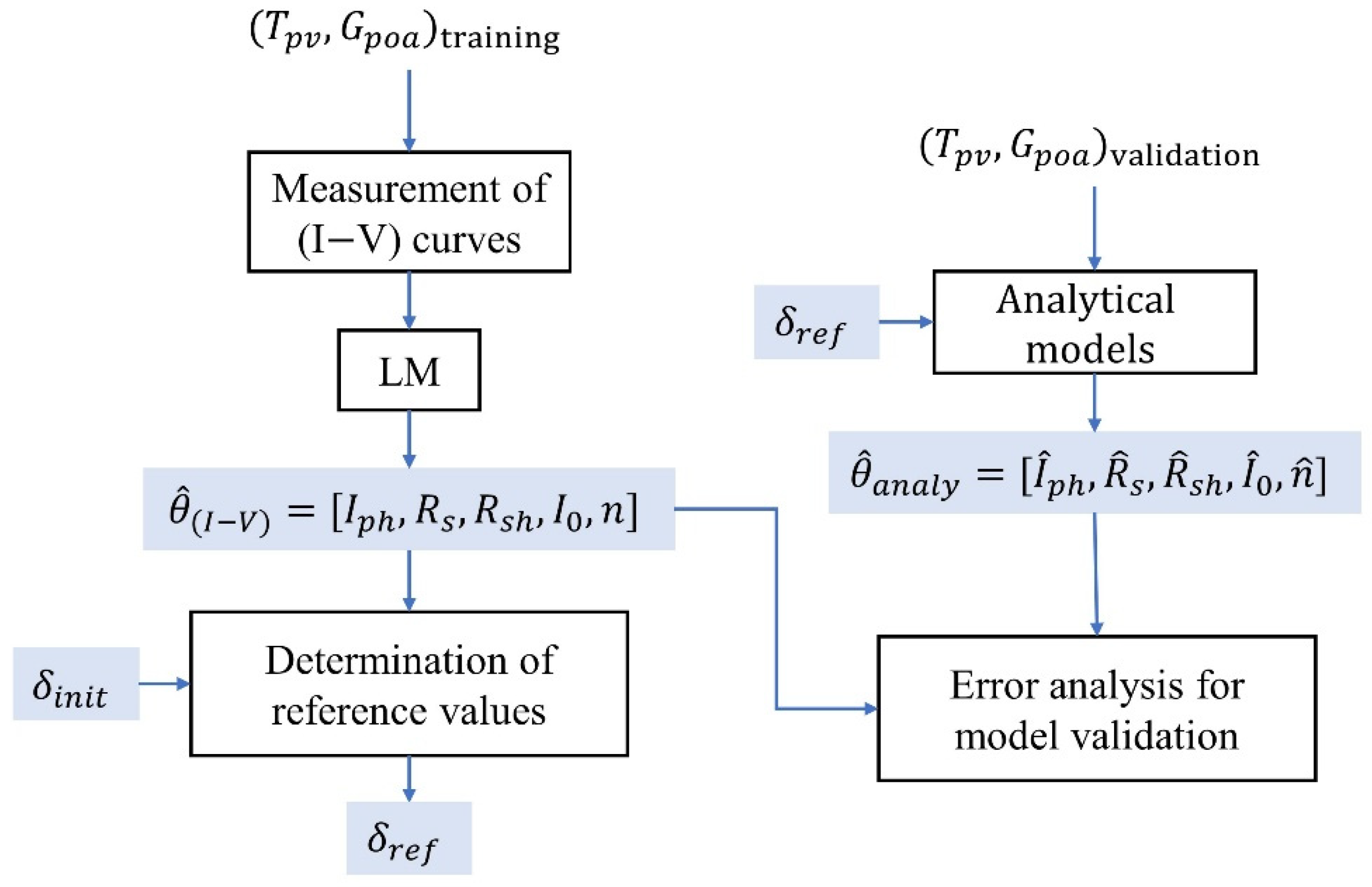
Energies 15 05350 g019aEnergies 15 05350 g019b
Figure 20. Flowchart to validate the hybrid PV model.
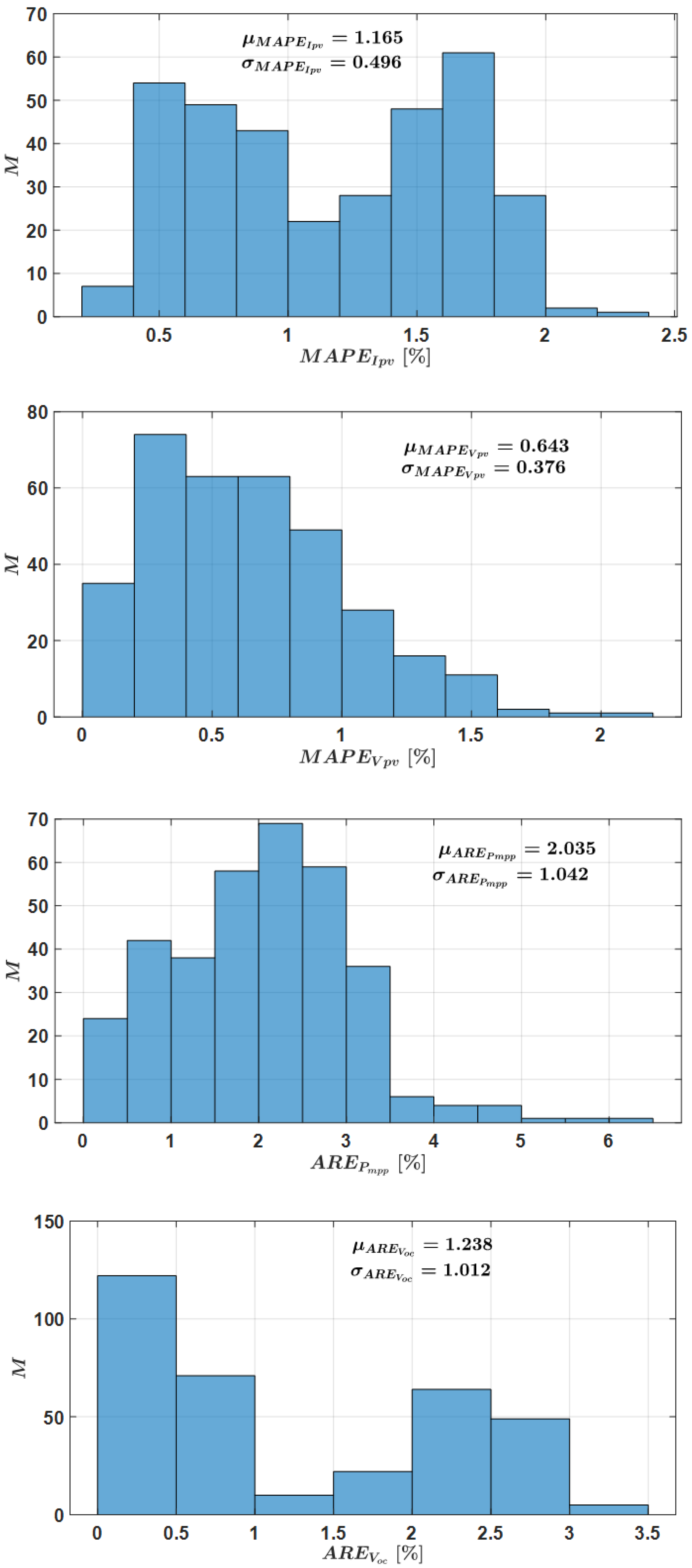
Energies 15 05350 g020
Figure 21. Histograms of the errors.
Energies 15 05350 g021aEnergies 15 05350 g021b
Figure 22. Flowchart of the FDD: (a) M1; (b) M2.
Energies 15 05350 g022
Figure 23. Histograms of Rs resistances.
Energies 15 05350 g023
Figure 24. Histograms of the residuals for Rs.
Energies 15 05350 g024
Figure 25. Effect of series resistance degradation on the other parameters of the SDM.
Energies 15 05350 g025aEnergies 15 05350 g025b
Figure 26. Effect of series resistance Rs faults on the I–V curve characteristics. (a): Fault effect on PV module’s current; (b): Fault effect on PV module’s voltage; (c): Fault effect on maximum power; (d): Fault effect on open-circuit voltage; (e): Fault effect on short-circuit current.
Energies 15 05350 g026aEnergies 15 05350 g026bEnergies 15 05350 g026c
Figure 27. FDD in the case of Rsh degradation. (a): Measured and estimated shunt resistance values; (b): Residuals.
Energies 15 05350 g027
Figure 28. Effect of Rsh degradation on the other parameters of the SDM.
Energies 15 05350 g028
Figure 29. Effect of shunt resistance fault Rsh on the I–V curve characteristics. (a): Fault effect on PV module’s current; (b): Fault effect on PV module’s voltage; (c): Fault effect on maximum power; (d): Fault effect on open-circuit voltage; (e): Fault effect on short-circuit current.
Energies 15 05350 g029aEnergies 15 05350 g029b
Table 1. Parameters under standard test conditions (STC), Gpoa = 1000 W/m2 and Tpv = 25 °C.
Electrical Performance under Standard Test Conditions (STC)
Maximum   Power   ( P m p p ) 87 W (+10%/−5%)
Maximum   Power   Voltage   ( V m p p ) 17.4 V
Maximum   Power   Current   ( I m p p ) 5.02 A
Open   Circuit   Voltage   ( V o c _ r e f ) 21.7 V
Short   Circuit   Voltage   ( I s c _ r e f ) 5.34 A
Temperature   Coefficient   of   V o c   ( k v _ r e f ) 0.37 % /°C
Temperature   Coefficient   of   I s c   ( k i _ r e f ) 0.038 % /°C
Table 2. Comparison with market I–V tracers.
TypeDuration of
Measurement
CostResolutionAcquisition MethodApplication
Proposed I–V tracer182 ms35 €26 pointsAuto and ContModule
Chauvin–Arnoux FTV 2000 IV tracer [21]-3650 €500 pointsManualModule
HT-Instruments I–V 500 W tracer [22]-4300 €128 pointsManual and AutoModule/String/Array
CHROMA Electronic load Model 63600 series [23] 2   μ s to 40 ms>4000 €1–4096 pointsManual and AutoModule/String/Array
EKO MP 11 IV checker [24]5 s-400 pointsManuel and AutoModule
HUAWEI Smart I–V tracer Diagnosis [25]1 s-128 pointsManual and AutoModule/String/Array
SOLMETRIC PV analyzer I–V tracer [26]0.05–2 s5468–11,038 €100 to 500 pointsManuel and AutoModule/String
Table 3. Data used for the training stage.
NoData AcquisitionWeatherNumber of I–V Curves
G p o a 600   W / m 2
12 September 2021Sunny94
28 September 2021Sunny86
310 September 2021Partly cloudy29
414 September 2021Partly cloudy45
515 September 2021Partly cloudy42
619 September 2021Partly cloudy44
720 September 2021Partly cloudy27
823 September 2021Partly cloudy58
924 September 2021Sunny63
Table 4. Extracted reference values for constant Tpv for the photocurrent model.
I s c _ r e f   [ A ] k i _ r e f [%/°C]
Initial value (STC)5.340.038
Optimized value5.8170.061
M A P E I p h 6.01%
Table 5. Extracted reference values for constant Gpoa for the photocurrent model.
I s c _ r e f   [ A ] k i _ r e f [%/°C]
Initial value (STC)5.8170.061
Optimized value5.7990.061
M A P E I p h 1.49 %
Table 6. Extracted reference values.
V o c _ r e f   [ V ] k v _ r e f [%/°C]
Initial value (STC)21.7−0.37
Optimized value20.68−0.519
M A P E I 0 7.34%
Table 7. Extracted reference values for constant Tpv for the series resistance model.
R s _ r e f   [ Ω ] β r e f
Initial value (STC)0.80.217
Optimized value0.7080.0359
M A P E R s _ r e f 0.88%
Table 8. Extracted reference values for constant Gpoa.
R s _ r e f   [ Ω ] β r e f
Initial value0.7080.0359
Optimized value0.7090.0359
M A P E R s _ r e f 0.92%
Table 9. Extracted reference value Rsh_ref.
R s h _ r e f   [ Ω ]
Initial value80
Optimized value49.85
M A P E R s h 7.4%
Table 10. Extracted reference value nref.
n r e f  
Initial value1
Optimized value1.01
M A P E n 0.58%
Table 11. Summary of the eight reference values extracted from the analytical models.
The Single Diode of PV Model with Five Electrical Parameters and Eight Reference Values
I p v = I p h I 0 [ e x p ( q ( V p v + I p v R s N s ) n N s K T K ) 1 ] ( V p v + I p v R s N s R s h N s )
Parameters of the SDMAnalytical ModelsThe Eight Reference Values
I s c r e f
[ A ]
k i _ r e f
[%/°C]
V o c r e f
[ V ]
k v _ r e f
[%/°C]
R s r e f
[ Ω ]
β r e f R s h r e f
[ Ω ]
n r e f
I p h I p h = I s c _ r e f [ 1 + k i r e f ( T p v T S T C ) ] G p o a G S T C 5.790.061------
I 0 I 0 = I s c _ r e f + k i r e f ( T p v T S T C ) e x p ( q V o c _ r e f [ 1 + k v r e f ( T p v T S T C ) ] n K N s T K ) 1 --20.68−0.519----
R s R s = R s _ r e f [ T K T n ( 1 β r e f ln ( G p o a G S T C ) ) ] ----0.7090.0359--
R s h R s h = R s h _ r e f G S T C G p o a ------49.85-
n n = n r e f T k T n -------1
Table 12. Data used for the validation step.
NoData AcquisitionWeatherNumber of I–V Curves
G p o a 600   W / m 2
13 September 2021Partly cloudy100
29 September 2021Partly cloudy21
312 September 2021Partly cloudy9
413 September 2021Partly cloudy42
522 September 2021Partly cloudy12
68 October 2021Partly cloudy44
79 October 2021Partly cloudy71
810 October 2021Partly cloudy56
911 October 2021Partly cloudy47
1015 October 2021Partly cloudy27
Table 13. Data for the validation of the hybrid PV model.
NoData AcquisitionWeatherNumber of I–V Curves
G p o a 600   W / m 2
13 September 2021Partly cloudy100
29 September 2021Partly cloudy21
313 September 2021Partly cloudy42
422 September 2021Partly cloudy12
58 October 2021Partly cloudy44
69 October 2021Partly cloudy71
710 October 2021Partly cloudy56
811 October 2021Partly cloudy47
Table 14. Data acquisition in case of Rs degradation.
NoData AcquisitionWeatherNumber of I–V Curves
G p o a 600   W / m 2
Fault Level
112 April 2021Partly cloudy38 Δ R s 3 = 0.39   Ω
217 April 2021Partly cloudy16 Δ R s 3 = 0.39   Ω
318 April 2021Partly cloudy56 Δ R s 3 = 0.39   Ω
419 April 2021Partly cloudy34 Δ R s 2 = 0.33   Ω
526 April2021Partly cloudy61 Δ R s 2 = 0.33   Ω
627 April 2021Partly cloudy61 Δ R s 2 = 0.33   Ω
720 April 2021Partly cloudy104 Δ R s 1 = 0.22   Ω
Table 15. Accuracy of fault level estimation in case of Rs degradation.
Fault Level f 1 f 2 f 3
Δ R s ( E x p e r i m e n t a l ) (Ω)0.220.330.39
Δ R s ( E s t i m a t e d ) (Ω)0.2050.3260.439
Relative error on Rs %1.570.374.35
Table 16. Effect of the Rs on the I–V curve characteristics.
Fault Level f 1 f 2 f 3
Δ μ M A P E I p v   ( % ) 1.41.841.99
Δ μ M A P E V p v   ( % ) 3.154.064.48
Δ μ A R E P m p p   ( % ) 3.64.645.1
Δ μ A R E V o c   ( % ) 0.130.210.32
Δ μ A R E I s c   ( % ) 0.010.0320.067
Table 17. Data acquisition for Rsh degradation.
NoData AcquisitionWeatherNumber of I–V Curves
G p o a 600   W / m 2
R s h _ a d d
113 April 2021Partly cloudy82 60   Ω
25 April 2021Partly cloudy61 50   Ω
33 April 2021Partly cloudy39 39   Ω
Table 18. Three levels of severity for Rsh degradation.
Fault Level R s h a d d
[ Ω ]
R s h m e a n , h
[ Ω ]
( Analytical   Model )
R s h m e a n , h / / R s h a d d Δ R s h   [ Ω ]
1 60 57.8929.4628.42
2 50 65.8128.41 37.39
3 39 63.824.20 39.59
Table 19. Fault effect on the I–V curve characteristics.
Fault Level f 1 f 2 f 3
Δ μ M A P E I p v   ( % ) 1.111.982.64
Δ μ M A P E V p v   ( % ) 0.190.310.66
Δ μ A R E P m p p   ( % ) 1.482.443.39
Δ μ A R E V o c   ( % ) 0.450.510.57
Δ μ A R E I s c   ( % ) 0.140.460.61
Table 20. Summary of FDD performance.
FDD MethodFault Types
R s   Degradation R s h   Degradation
M1 I p h No effect I p h No effect
R s High R s No effect
R s h No effect R s h High
I 0 No effect I 0 No effect
n No effect n No effect
M2 I p v Low I p v Low
V p v Low V p v Low
P m p p High P m p p High
V o c Low V o c Low
I s c Low I s c Low
Publisher’s Note: MDPI stays neutral with regard to jurisdictional claims in published maps and institutional affiliations.

