1. Introduction
Microgrids are evolving to become fundamental building blocks in a smart grid, and their proliferation has incentivized utilities to revisit the existing grid management paradigm. Since microgrids (MGs) are controllable entities consisting of interconnected loads and distributed energy resources (DERs), effective energy transfer and coordination between them could help maintain the stability and reliability of regional large-scale power grids. For this reason, in the past two decades a considerable amount of research has been devoted to the design and management of MGs. The IEEE Power and Energy Society task force on MG control has provided a comprehensive review of recent results in this field (see [
1] and the references therein).
Connecting multiple MGs can provide additional operational flexibility for large-scale power grids, since it allows them to realize the benefits of variable DERs more effectively. In order to accomplish that, MGs within a region must cooperate with each other in a way that improves efficiency, reliability, and resilience. This means (among other things) that interconnected microgrids should not limit their exchanges to energy generated by renewable sources and should also share energy that is accumulated in their storage devices. Such an approach can improve the local supply and demand balance for each individual microgrid, resulting in a more reliable power supply for consumers. This objective has become increasingly important in light of recent natural disasters in the USA, which have underscored the need to prioritize resiliency over operation costs.
Basic control architectures for multiple microgrids can be categorized as centralized, decentralized, distributed, and hierarchical [
2]. This work will focus on distributed control where
both local measurements
and information from neighboring units are utilized. The main challenge in this case is how to achieve optimal coordination among the subsystems.
This problem has attracted considerable attention in recent years, and a large body of research has been devoted to the potential benefits that can arise from the coordinated operation management of neighboring microgrids [
3]. The solutions that have been proposed so far take many different forms and depend on the types of MGs that are involved, their sizes, and their proximity. A group of MGs that are geographically close and are physically interconnected via dc (or ac) buses is referred to as a
microgrid cluster [
4]. Such clusters typically allow for the maximal utilization of energy sources and can improve reliability. There is a growing interest in such microgrids, due in a large part to the increasing number of dc sources and loads.
Multilevel control schemes are widely accepted as a standard solution for the efficient energy management of multiple MGs. The first of these levels (which is known as primary control) is responsible for regulating local voltage and frequency. It normally follows the set-points provided by higher level controllers and performs control actions over interface power converters. Secondary control deals with system-level issues, such as power quality regulation, the synchronization of MGs with the external network, the coordination of distributed generation, and so on. Tertiary control is tasked with optimization, management, and overall system regulation. It should be noted in this context that primary and secondary control levels are associated with the operation of individual MGs, while tertiary control pertains to the coordinated operation between MGs and the utility grid [
1].
Most existing papers on distributed tertiary control focus on enhanced efficiency and balanced power flow between the MG and the utility grid, taking into account optimality, stability, and economic factors. The distributed power management between MGs within a cluster has also been studied (see, for example, [
5,
6,
7,
8,
9,
10,
11] and the references therein). It is interesting to note, however, that only a handful of papers have examined MG clusters as a possible way to cope with the intermittence and randomness of renewable energy [
12,
13,
14,
15,
16,
17,
18,
19]. Some of the most recent work on this subject considers a hierarchical control scheme and a corresponding consensus-based multilayered event-triggered control algorithm for MG clusters [
20]. There have also been some new results related to distributed optimization at the MG cluster level [
21], and the problem of distribution load sharing [
22].
Although these references offer a variety of different approaches, there is a general agreement that stability and reliability can be greatly improved by connecting MGs directly to the utility grid, or by forming clusters of interconnected MGs [
23]. In view of that, in this paper we propose a distributed control strategy for MG clusters that operate in the islanded mode. What makes this strategy unique is the fact that it simultaneously addresses two different types of uncertainties in the system: the inherent randomness of renewable generation (such as solar energy), and unpredictable changes in the system topology that can arise as a result of natural disasters and/or extreme operating conditions. The main advantages of this approach can be summarized as follows:
- (1)
The dynamic model that is proposed is linear and hybrid. It incorporates the stochastic nature of renewable sources and can accommodate arbitrary energy exchange patterns between the MGs. Such a model is required in order to analytically determine the control gains, and its simplicity ensures that the necessary computations can be performed efficiently.
- (2)
An optimal control strategy is developed to maximize the energy storage of each MG. This is accomplished by regulating the power flow between MGs using a modified version of the so-called
ε-suboptimality theorem [
24], which is suitable for large-scale systems. This result allows for arbitrary interconnection patterns between MGs and guarantees a desired level of suboptimality in all cases.
- (3)
The control law (which is based on the jump linear theory [
25]) is designed to ensure stability under structural perturbations, while minimizing the error between the load demand (set point) and generation.
- (4)
The gain matrix can be calculated offline for all relevant generation patterns. We can do so analytically using the proposed dynamic model, and the necessary computations can be performed in a multiprocessor environment (since each gain matrix is determined independently). Something similar can be said for computations related to ε-suboptimality, which can be performed efficiently even when the system is large (due to the special structure of the dynamic model).
The paper is organized as follows. In
Section 2, we present a simplified model for flexible MG clusters that takes into account power exchanges between MGs. We then proceed to develop a stochastic optimal control strategy, which is described in
Section 3. In
Section 4, we explain how the
ε-suboptimality theorem can be used to achieve maximal power transfer between MGs. Simulation results and their analysis are provided in
Section 5. Since the example that we consider serves primarily as a proof of concept, we focused on clusters that contain less than five MGs and have a peak load of less than 10 MW. This assumption is not necessary from a theoretical standpoint, but it has some practical benefits when it comes to simulation. We conclude with a discussion of the potential advantages of this approach and a brief overview of future directions for future research.
2. System Description and Mathematical Modeling
We begin this section by offering a general system description for multiple interconnected MGs. We will then introduce a simple mathematical model that represents an extension of the one proposed in [
26]. This model will be utilized to develop a stochastic multivariate optimal control strategy, whose objective is to address some recent challenges in the energy management of multiple MGs. As noted in the Introduction, we will focus on interconnected MGs that are disconnected from the utility grid and are geographically close to each other.
2.1. System Description
Figure 1 provides a schematic representation of multiple MGs that can exchange energy with each other in an arbitrary manner. Although the microgrids in this diagram are disconnected from the utility grid, we should point out that the connection can be reestablished whenever that becomes necessary. The MGs are concentrated in a relatively small geographic area and are connected to a common bus through a static switch. In configurations of this sort (which are known as clustered MGs), it is assumed that each subsystem can share its energy needs via a communication network. This assumption is realistic in a smart grid since smart meters are capable of broadcasting data over a network.
Throughout this study, we will distinguish between two modes of operation—The
interconnected mode (in which multiple MGs can exchange energy) and the
disconnected mode, in which this is not possible. The latter configuration (and the one where MGs are connected to the utility grid) was considered in our previous work [
26] and will be used here only for comparison purposes. Our objective in this paper will be to achieve optimal energy management of interconnected multiple MGs by maximizing the battery storage capacity usage, as well as the utilization of solar energy.
Since the focus of our work is distributed tertiary control in a hierarchical architecture, a continuous dynamic model for structures of this type will be proposed in the next section. We will concentrate primarily on commercial MGs (including university campuses), since systems of this sort have two important features that allow us to develop an effective and robust control strategy:
Although each MG load can be comprised of multiple buildings (with varying energy demands), its aggregated power has a predictable profile.
The load demand reaches its peak during the day (when solar energy is typically available) and becomes minimal at the end of the day as residential loads start peaking.
In modeling the dynamic behavior of MGs, we will assume that each MG can be connected to or disconnected from the cluster in a random manner, depending on its load, its generation needs, and its ability to share energy. In the proposed model, individual MGs are controlled using locally available information, while energy exchanges are based on global information. The control law must ensure that stability (and an acceptable level of suboptimality) is retained for
all possible interconnection patterns. Closed loop systems that have this property are said to be
connectively stable [
24].
In the model that we will be working with, each MG consists of a specific load (commercial or a university campus), battery storage, and an array of solar cells. When it is in the disconnected mode, solar energy is provided internally, and is distributed to the battery and the load in a way that reflects the load requirements. During the night, it is assumed that the battery is the sole source of energy. This is a reasonable assumption, since most large commercial consumers require less energy during the night than during the day. In situations where the required battery storage is not available, a secondary dispatchable generation source (such as a fuel cell, for example) may be considered. We should point out, however, that such additions have little effect on our control strategy, so we will disregard them in our analysis. When MGs operate in the interconnected mode, each of them can deliver power to other MGs provided that their own load requirements are satisfied. The shared energy can then be used to charge the batteries of microgrids whose storage levels are not sufficiently high.
2.1.1. The Load Model
In the simplified scenario that we just described, the primary goal is to manage the energy demand in a system that consists of
n microgrids. This is done by balancing the real power generated by the PV array (
) and the battery (
) in MG
m with the power required by the load (
, and the power that MG
m exchanges with other MGs (which will be denoted in the following by
). Note that
will be positive if MG
m delivers energy to the network, and negative if this microgrid absorbs energy. Using this notation, we can express the power balance as:
where parameter
represents the fraction of solar power that is delivered to the load (the value of this constant is chosen based on the solar panel size and battery storage capacity). As we already mentioned, it is assumed that
follows a known deterministic trajectory, and the power generated by the PV array,
will be treated as a random variable whose characteristics depend on cloud coverage and the time of day. Since the battery can inject power into the system (as well as absorb it when needed), we will treat
as a control input.
Power losses that are primarily due to transmission lines are neglected in this model, since MGs that belong to the same cluster are considered to be close to each other (by definition). The PV array should be sized in a way that is proportional to the daytime peak load requirements (which is becoming increasingly feasible due to the decreasing cost of solar panels). This ensures full load satisfaction when the weather is sunny. The battery should also be properly sized so that it can meet the night load. Because the excess energy produced by the array can be used to charge the battery, the battery can act as a buffer. This allows the system to use the stored solar energy when the PV array is inactive.
In addition to the relationship described in (1), our model incorporates the following four assumptions:
Information about the system state (which includes instantaneous power flows, maximal and minimal generation levels, and maximal and minimal battery levels) is readily available. This can be ensured by using a battery state of charge (SoC) tracker, combined with voltage, current, or phasor monitoring devices.
Only active power is considered, and it is assumed that the controllers/inverters on the PV array and battery regulate voltages and phase angles.
The data used to represent the commercial load for each MG corresponds to the typical commercial load in the US. This data are provided by National Renewable Energy Laboratory (NREL) and is available online [
27].
Changes in solar generation states are detected via solar radiation sensors.
2.1.2. The Solar Generation Model
Although solar power is a highly desirable form of generation, it has certain intrinsic shortcomings that stem from its intermittent nature. To model the stochastic character of solar generation, a continuous Markov chain will be used to represent different levels of cloud coverage. The details of this model are discussed in [
26], so we will only highlight its most pertinent features.
In general, cloud coverage classification should be based on regional weather patterns. This means that the number of relevant scenarios can vary significantly, depending on where the MG cluster is located. The model that we propose allows for this type of flexibility, but in our simulations we will concentrate on a somewhat simpler case, which reflects the weather patterns in northern California. According to the data obtained from the San Jose International Airport meteorological report [
28], in northern California it suffices to consider only three different levels of cloud cover: sunny, partly cloudy, and overcast.
At night there is obviously no generation, so the power produced by the PV array,
can be represented as a piecewise constant function (where
at night and
during the day). The term
denotes the state of the Markov chain that corresponds to the cloud coverage during the day. This means that
r(
t) evolves according to a continuous time Markov chain [
22,
28], taking values from set
in the geographic region that we are concerned with.
Matrix
P =
which characterizes this process, provides the probabilities of transitioning from one state to another, and its elements are given by:
where
and
. In this expression, coefficients
represent the (non-negative) transition rate from
i to
j (
, and
is defined as
Given this notation, the transition rate matrix
will have the form
[
25].
The transition probability matrix and the transition rates that were used in our simulations were calculated from the data set provided in [
28] (which contains information gathered between 2008 and 2017). An analysis of this data indicates that the transition probabilities do not change significantly from year to year. As a result, we can assume that the corresponding matrix is fixed for microgrids located in northern California.
2.1.3. The Battery Model
Each microgrid is assumed to have a battery storage system that supplements the intermittent generation from the PV array. Relevant battery characteristics include its energy capacity (more specifically SoC), its charge/discharge powers, its life cycle, as well as its safe operating temperatures. In the following, we will assume that the energy stored in the battery, , and the charge/discharge power can be used to provide adequate information about the SoC.
The battery is assumed to have energy limits,
, and variations in the stored energy can be described as [
29]
In this expression, , denotes the rate of self-discharge, and is the battery discharge. We will assume that batteries have the same efficiency when charging and discharging, and that they can easily switch from one mode to the other (this feature becomes important in cases when MGs exchange energy directly). For normal battery operation, it is common to set its upper and lower energy limits to 10% and 90% of the maximum energy that can be stored. By doing so, we can increase the lifespan of the battery.
2.2. Mathematical Modeling
Combining Equations (1) and (4), the energy management of MG
m in a system made up of
n MGs can be described as:
In this expression it is implicitly assumed that there are no energy exchanges with the utility grid since we are interested only in the islanded mode of operation. If MG
m has unused energy that it can share, we can represent
as
, where
is the amount of energy that MG
m has delivered to other MGs during the interval
(
being the time when the exchange begins). Since we have the freedom to decide how the energy exchanges are scheduled, we will assume that this is done in such a way that
is proportional to the amount of energy consumed by the load
m up to time
. That allows us to express
as
where
determines the fraction of
that is transferred from MG
m to MG
k (note that these coefficients have the appropriate units). Since coefficients
are adjusted based on the varying energy needs of each microgrid, we will treat their values as uncertain quantities. In the sections that follow, we will explain the constraints that these values must satisfy in order to ensure a desired level of suboptimality.
When microgrid
m delivers power to other MGs,
will have the form shown in Equation (6). Setting
and recalling that
, Equation (1) becomes
In cases when MG
m receives power from other MGs,
is negative, and can be expressed as
Under such circumstances, Equation (1) takes the form
Since a microgrid can either deliver or receive energy, Equations (8) and (10) represent the only possible scenarios for a given MG. This includes situations where certain MGs are disconnected (since we can treat them as a special case of (10) where for all k).
One of the principal advantages of the proposed model is that the system can be stabilized using decentralized control
regardless of how coefficients are chosen. In order to demonstrate that, suppose that
q MGs are absorbing power at some point in time, and that
are delivering. We can always number the MGs in such a way that the ones that absorb power come
first. For any such MG, we have that
, and the power balance equation has the form
For MGs that deliver power, we have that
and
Introducing matrices
and defining vector
, the
n subsystems can be represented as
for
, and
for
. The overall interconnected system can then be described as
where matrix
A has an upper block triangular structure
and
In this system of equations, denotes the state vector, represents the control action (which is implemented by charging and discharging batteries), and vector P(t) is the power delivered by the solar panels (a part of which goes to batteries).
The fact that matrix
is upper block triangular is of crucial importance here, because it ensures that the stability of the individual subsystems implies the stability of the overall system. Note that this will be the case regardless of how the microgrids are actually numbered—for stability purposes, it suffices to recognize that a permutation that produces the structure in (17)
exists for every possible energy exchange pattern. A more general scenario where existence is not guaranteed is described in [
30]. In this case, it is necessary to use an efficient decomposition algorithm that can determine an appropriate decentralized control law.
In the worst-case scenario (from a stability perspective), block
will have the form
(blocks of this sort correspond to MGs that are receiving energy). We can easily stabilize any such subsystem ahead of time using decentralized control. As a result, we can ensure that the overall system will be stable for
any set of coefficients
that we choose.
2.3. Microgrid Exchange Protocol
In addition to ensuring stability for arbitrary energy exchange patterns, it is also necessary to develop a systematic procedure that all such exchanges must follow. With that in mind, we propose the following simple scheme:
- (a)
Each MG that
delivers energy sends an amount equal to
to the common bus (see
Figure 1).
- (b)
Each MG that
absorbs energy takes
from the common bus.
If we adopt this approach, the energy that an individual MG sends through the common bus can be aggregated (which is convenient from a practical perspective). Note, however, that its contribution is uniquely defined by the value of coefficient . The same can be said for the energy absorbed by an MG that requested additional resources, which is determined by coefficients . As a result, the proposed strategy can be easily implemented.
3. Stochastic Control Strategy for Interconnected MGs
Since the system matrix
is always permutable into an upper block triangular form, we have the flexibility to consider a range of possible decentralized control strategies. Given the random nature of solar generation, it would be logical to incorporate stochastic elements into the process for determining the gain matrices. We propose to do so by representing solar generation as a continuous Markov chain and applying jump linear quadratic control to each microgrid (following the ideas introduced in [
26,
31,
32]).
Our principal design objective will be to produce a different gain matrix for each level of cloud coverage and ensure that the load demand is satisfied in all cases. Because each of these scenarios is independent (and can be handled offline), the computation of the gain matrices can be distributed across multiple processors. This obviously contributes to the computational efficiency of the procedure and makes the design safer with respect to potential cyber-attacks (since each subsystem can compute its own gain matrices locally).
In order to describe the proposed control design, we will first provide a brief overview of jump linear systems and optimization techniques that are suitable for them. We will then apply this methodology to interconnected microgrids, where the cost function is defined in terms of deviations from the load demand.
3.1. An Overview of Jump Linear Systems Tracking Problem
The state–space representation of a jump linear system (JLS) for a tracking problem has the general form
with
, where
and
are
and
matrices, respectively, and
denotes the current system mode (which is determined by a finite state Markov jump process). To simplify the notation, in the following we will refer to matrices
as
and
as
when the system operates in the
ith mode [
25]. Since
reflects the cloud coverage during the day, this variable evolves according to a continuous time Markov chain. When designing an optimal controller for such a system, one aims to minimize the quadratic cost function:
where
t0 and
tf denote the initial and final time, respectively, and E{.} represents the expected value of a random function [
25]. The symmetric weighting matrices,
, are mode dependent and are used to tune the system response to fit desired characteristics. In the following, they will be denoted as
with
(positive semi-definite) and
(positive definite) when the system is operating in its
ith mode.
In this paper, we will be primarily interested in the ergodic infinite horizon problem and the steady state values of the control gain. The cost function
is minimized using the stochastic maximum principle, which produces a time-varying feedback control law affine in state of the form:
where matrices
satisfy the set of coupled algebraic Riccati equations
with
.
Under stochastic controllability and observability conditions [
32], the Riccati gains for the infinite horizon problem will converge to the unique positive definite solutions of the coupled algebraic Riccati equations. Equations of this sort can be solved using the numerical algorithm proposed in [
33]. The bias vector
in (23) satisfies
, and evolves according to equation
The term
should be interpreted as the change in the operating points due to the fact that system transitions from mode
i to mode
j [
31,
34]. In this particular case, it is equal to
. In the steady state,
can be easily computed by solving three equations in three unknowns once (24) is solved.
3.2. JLQC Strategy for Interconnected Microgrids
Before we apply this approach to interconnected microgrids, we should first recall that energy exchanges between them are dictated by the needs of each individual MG. Since these needs can vary unpredictably for a given state of cloud coverage, coefficients cannot be known in advance. With that in mind, we will perform the optimization on individual microgrids when they are disconnected from each other (in which case for all m and k).
If we treat the solar energy production of microgrid
m as a continuous Markov chain, the power delivered will be a piecewise constant, with the changes coinciding with jumps (it is assumed that these changes can be easily detected via solar radiation sensors). Under such circumstances, microgrid
m can be viewed as a continuous linear time invariant system with Markovian jumps and a hybrid (continuous–discrete) state space
. The corresponding state space model will have the general form
where matrix
differs from one state of solar energy to another. Note that matrices
do not appear in this equation, because the optimal control is designed under the assumption that all coefficients
are zero. We should also point out that matrix
does not depend on solar generation states, and therefore has no superscript associated with it.
Since this paper focuses on power system resiliency, our main objective in the following will be to optimize battery storage while satisfying the load demand when the MG clusters are in an islanded mode. Such an optimization requires a cost function that reflects the mismatch between the demand and the power delivered. This function will also have to take into account random variations in solar generation, which are due to changes in cloud coverage. In order to meet these criteria, it will be necessary to introduce a change of variables [
23], in which case the subsystem model becomes
where
and
In expression (29),
represents the desired energy setpoints for the battery and the load (which are mode dependent in general). Set point changes are designed to address two types of variations in the system: the discrepancy between the load demand during the day and at night, and fluctuations in power generation due to different cloud coverages. The vector
that appears in (28) is related to
as
For the infinite horizon problem with performance measure
(where
), the optimal discharge and charging patterns of the batteries is obtained by minimizing function
J. This ensures that the error between the generation and the demand is as small as possible. The resulting optimal regulator is given as a time-varying feedback law
It is important to emphasize once again that this gain matrix is independent of coefficients , since it is designed to optimize decoupled microgrids. As a result, the corresponding decentralized control laws can be computed offline for any given level of cloud coverage.
4. Suboptimality and Energy Exchanges
Since the optimal control law described in the previous section is designed to minimize cost function
J when all subsystems are decoupled, we now need to consider what happens when the microgrids are allowed to exchange energy. In that case, coefficients
will assume nonzero values, and the system will become
suboptimal. If we denote the minimal value of the cost function in the disconnected mode by
, this means that
(which corresponds to the case when subsystems are connected) will necessarily be larger. The following definition provided in [
24] allows us to compare these two scenarios and evaluate the degree of suboptimality in the system.
Definition 1. Let
denote the optimal value of the cost function in the disconnected mode, and let
be the value that corresponds to the interconnection pattern
k. The system is said to be
suboptimal with index ε if
Since suboptimality is a result of the interactions between the subsystems, index
ε will obviously depend on their magnitude. Conditions that ensure the existence of such an index are provided in Theorem 1, which represents a straightforward application to the result provided in [
24].
Theorem 1. The system described by Equations (14) and (15) withis suboptimal with index ε if:whereare the minimal and maximal eigenvalues of the respective matrices, and In (35), Km denotes the optimal gain matrix for subsystem m, while Qm and Rm represent weighting matrices. Since Km is calculated based on the choice of Qm and Rm, these two matrices can be viewed as tuning parameters that allow the system to meet certain additional constraints. In the case of microgrids, the relevant constraints are defined by the upper and lower limits on battery storage levels, and the requirement that the load demand must be met in each subsystem.
In order to apply this result to jump linear systems, we need to modify Theorem 1 in the following way.
Theorem 2. The system described by Equations (14)
and (15)
with is suboptimal with index εi ifwhere are the minimal and maximal eigenvalues of the respective matrices for each state i of the Markov chain, and is given as As in the case of Theorem 1, the proof follows directly from the results provided in [
24]. What makes this result particularly useful is the fact that it provides a simple upper bound for coefficients
. These coefficients need to be adjusted every time one of the microgrids requests additional energy, so it is important to determine an appropriate exchange pattern quickly. We can do so because matrices
and
are computed
ahead of time for each level of cloud coverage. This allows us to treat the right-hand side of inequality (38) as a known function of
ε at the point when we need to choose new values for coefficients
.
Remark 1. It is important to recognize that the results described in this section remain valid regardless of how the cost function is chosen. It is therefore possible to adapt the proposed procedure to other types of constraints (such as those related to energy production or economic impact, for example). We intend to address this possibility in our future work.
5. Simulation Results
In this section, we provide simulation results that were obtained using cloud coverage data from San Jose International airport [
28], load data from NREL [
27], and the Santa Clara University feeder. To keep the analysis as simple as possible, we considered a cluster of three microgrids, which can operate in the connected or disconnected mode, and can have different types of solar panels and battery storages. We assumed that one of the microgrids represents a university, and that the other two correspond to commercial MGs. Theorem 2 and the exchange protocol described in
Section 2.3 were used to calculate the maximal amount of energy that can be transferred given a desired level of suboptimality.
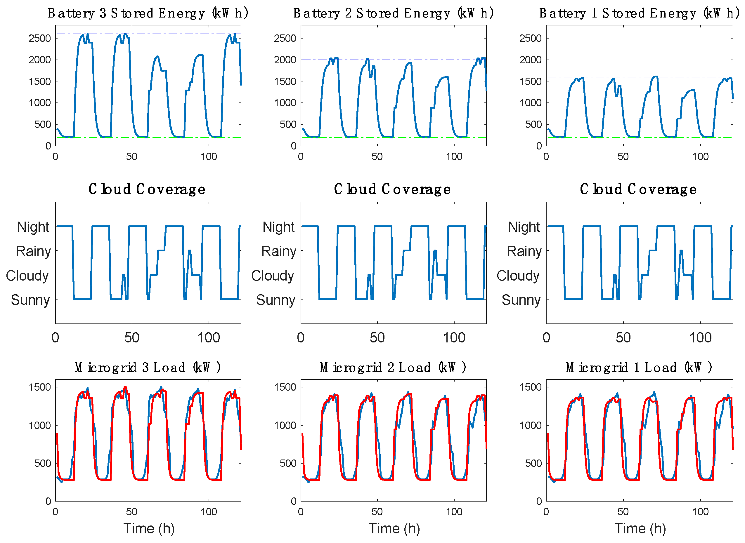
For simulation purposes, we assumed that the battery storage and PV array of MG 3 are large enough to satisfy its own needs, and that the excess energy is shared with MGs 1 and 2. To better illustrate the potential benefits of the proposed approach, we additionally assumed that the battery storage and PV arrays for these two MGs do not produce enough energy to meet the demand at all times. Data from [
28] were used to generate random cloud coverage patterns by Monte Carlo simulations, which determined the overall amount of solar generation at any given point in time.
Following the discussion in
Section 1, we divided cloud coverage levels into three categories (which is representative of the weather pattern in northern California).
Figure 2 provides the step-by-step procedure used to design the optimal regulator and calculate coefficients
.
The results that we obtained are shown in
Figure 3 and
Figure 4 (they cover a period of 5 business days). Since commercial load behavior is relatively predictable, we were able to use the load profile as a collection of setpoints instead of treating it as an input or a disturbance. In that respect, our approach differs from most other methods described in the literature. We should also note that due to the low or zero inertia related to batteries and solar energy, small imbalances between the supply and demand can be handled by batteries and PV arrays (or additional DC sources).
Figure 3 shows the simulation results for the three microgrids when they are in the
disconnected mode. It is readily observed that all three batteries discharge to their lower limit at night, and that batteries in MGs 1 and 2 are unable to fully charge even when the weather is sunny (since their PV arrays are not sufficiently large). We should also point out that the load demands in MGs 1 and 2 (which are marked in blue in the bottom figure) are
not met during peak hours.
The graphs in
Figure 4 correspond to the situation where the three MGs are interconnected and can specify their needs through a communication network. When the demand in MG 3 is met and its battery is sufficiently full, energy is transferred to MGs 1 and 2. During these intervals, batteries 1 and 2 are able to charge.
To highlight the potential advantages of this approach, we considered a scenario where MGs 1 and 2 were able to fully satisfy their internal demand using the energy provided by MG 3. If this were not the case, MGs 1 and 2 could always connect to the utility grid and request the additional power that they need [
26] (or possibly use a secondary source of generation). It is important to recognize, however, that the proposed scheme is helpful in such cases as well, because it reduces the amount of additional energy that is required. To evaluate the impact of energy exchanges in the latter scenario, we computed the integral of the mismatch between the demand and supply over a five-day period. We found that the total error was reduced by about 8 MW, which is significant.
6. Conclusions
In this paper, an optimal distributed stochastic control strategy was proposed for the energy management of MG clusters. A power balance model was developed that takes into account not only the randomness of solar generation, but also the exchange of power between MGs. The ε suboptimality index was used to compute the maximal amount of energy that any MG can deliver or absorb for a given choice of ε. Simulation results using real data were provided for a cluster with three MGs.
The proposed approach was found to have the following advantages:
- (1)
Although it incorporates random variations in solar generation into the controller gains, it does not require an iterative algorithm to calculate the gain matrix. Because of that (and because all of the computations can be carried out offline), this method is suitable for real-time implementation.
- (2)
It allows the user to determine upper limits for the power exchange, based on the controller design. These limits were shown to be independent of the way in which the MGs are connected.
- (3)
The resulting decentralized control scheme guarantees stability for all possible interconnection patterns (as shown in
Section 2.2).
- (4)
All the main features of this method can be easily adapted to networked MGs, since there is no restriction on how large n can be.
In our future work, we will consider possibilities for further improvement (such as incorporating the demand response into the model and considering different types of cost functions). We will also relax the assumption that the microgrids are physically close to each other, and that their loads have a known profile.


