
Optimal Scheduling Model of a Battery Energy Storage System in the Unit Commitment Problem Using Special Ordered Set


Abstract
:1. Introduction
2. Previous Studies
3. Modeling
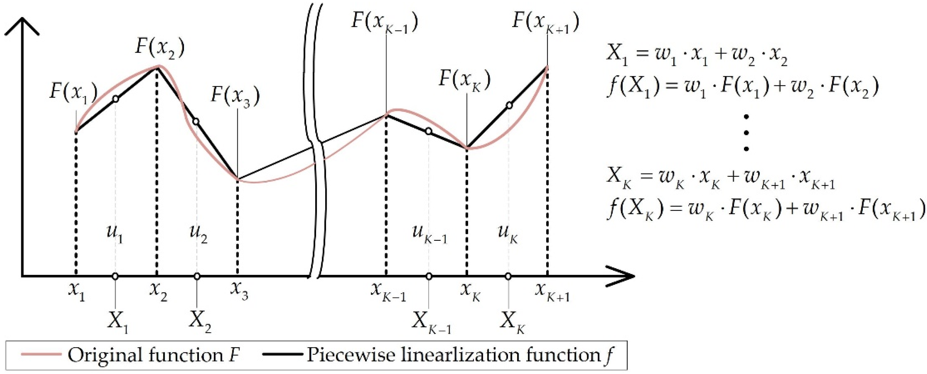
3.1. Special Ordered Set of Type 2
3.2. BESS Operation Constraint
3.3. Unit Commitment
4. Case Study
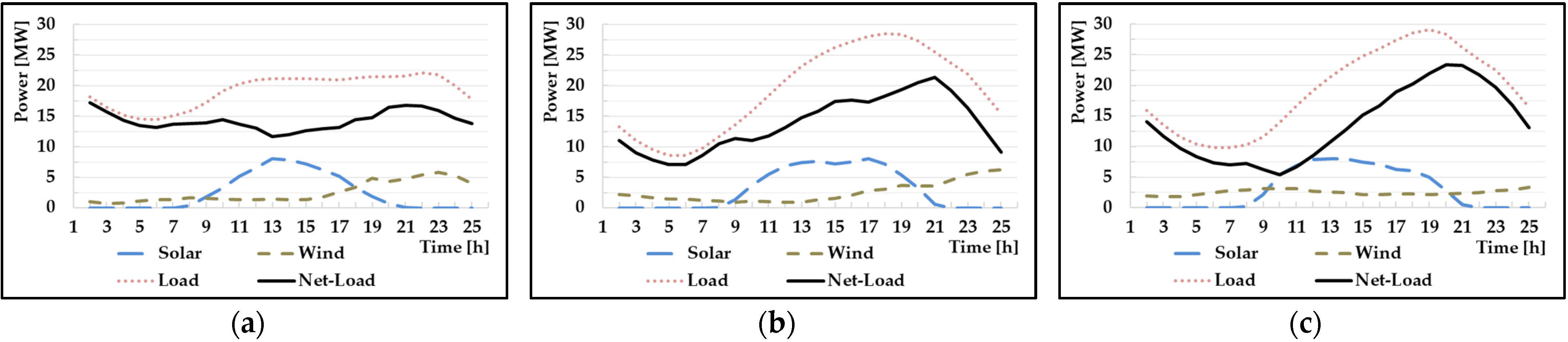
4.1. Scenario Data
- -
- Method I: assume that , , and are constant
- -
- Method II: proposed method using SOS2
- -
- Method I70: , = 70%
- -
- Method I80: , = 80%
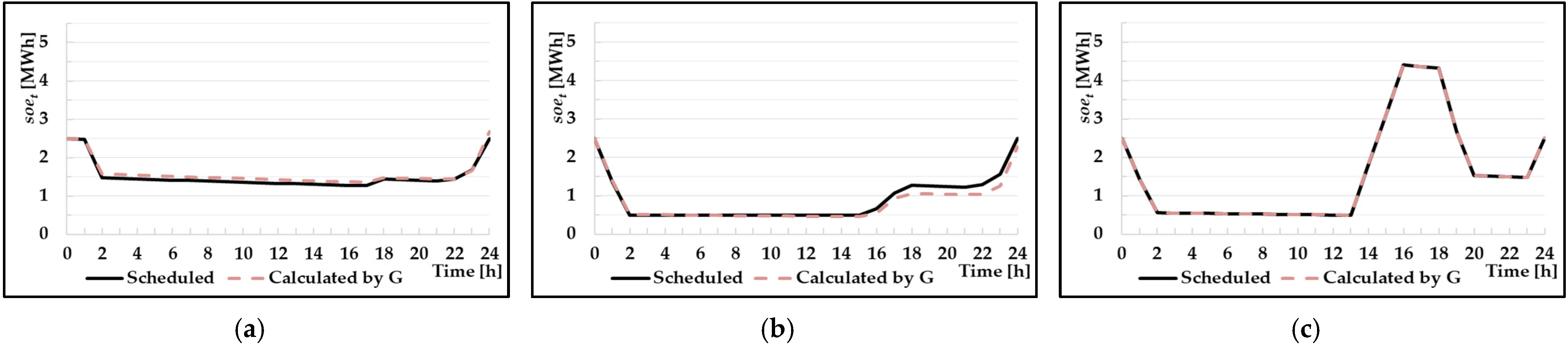
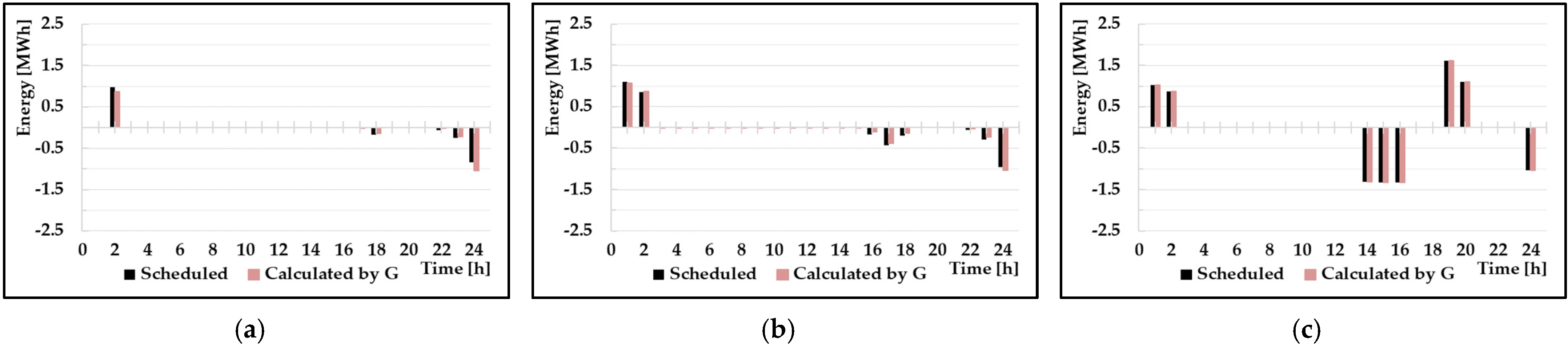
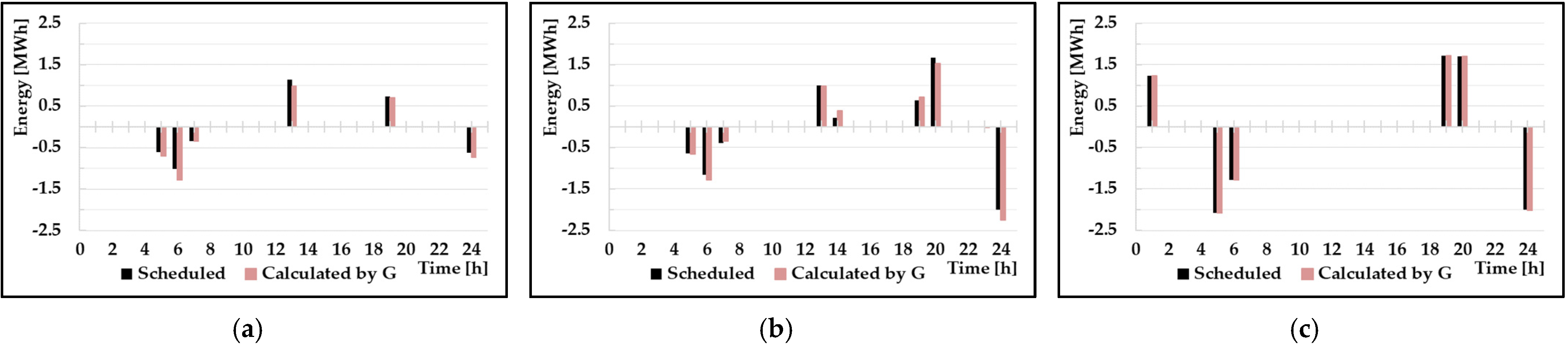
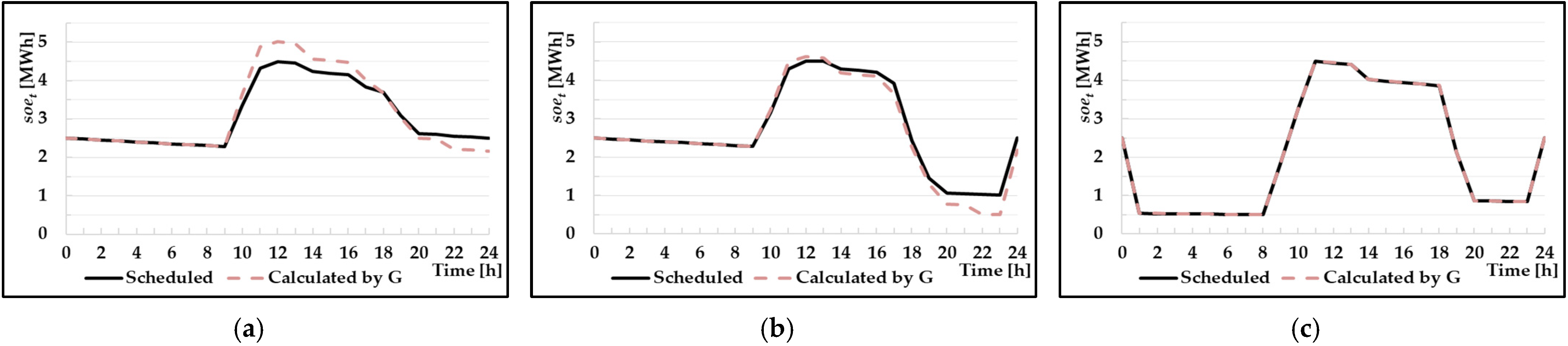
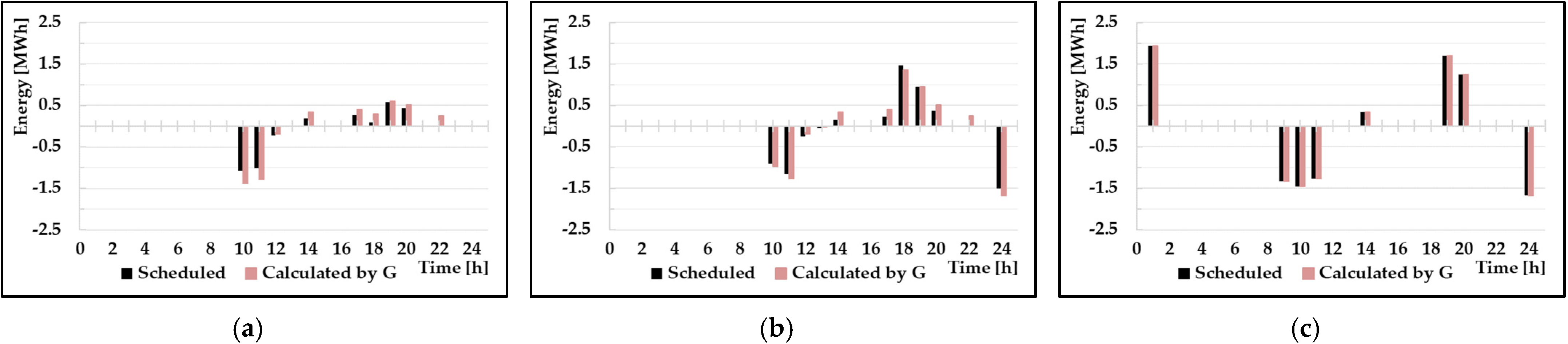
4.2. Results
5. Conclusions
Author Contributions
Funding
Institutional Review Board Statement
Informed Consent Statement
Data Availability Statement
Conflicts of Interest
References
- Etxeberria, A.; Vechiu, I.; Camblong, H.; Vinassa, J.M.; Camblong, H. Hybrid Energy Storage Systems for renewable Energy Sources Integration in microgrids: A review. In Proceedings of the International Power Engineering Conference (IPEC), Singapore, 27–29 October 2010. [Google Scholar]
- Lobato, E.; Sigrist, L.; Rouco, L. Use of energy storage systems for peak shaving in the Spanish Canary Islands. In Proceedings of the IEEE Power & Energy Society General Meeting, Vancouver, BC, Canada, 21–25 July 2013. [Google Scholar]
- Li, Y.; Yang, Z.; Li, G.; Zhao, D.; Tian, W. Optimal Scheduling of an Isolated Microgrid with Battery Storage Considering Load and Renewable Generation Uncertainties. IEEE Trans. Ind. Electron. 2019, 66, 1565–1575. [Google Scholar] [CrossRef] [Green Version]
- Chowdhury, A.H.; Asaduz-Zaman, M. Load frequency control of multi-microgrid using energy storage system. In Proceedings of the 8th International Conference on Electrical and Computer Engineering, Dhaka, Bangladesh, 20–22 December 2014. [Google Scholar]
- Lee, Y.D.; Jiang, J.L.; Su, H.J.; Ho, Y.H.; Chang, Y.R. Ancillary voltage control for a distribution feeder by using energy storage system in microgrid. In Proceedings of the 2016 IEEE 7th International Symposium on Power Electronics for Distributed Generation Systems (PEDG), Vancouver, BC, Canada, 27–30 June 2016. [Google Scholar]
- Faisal, M.; Hanan, M.A.; Ker, P.J.; Hussain, A.; Mansor, M.B.; Blaabjerg, F. Review of Energy Storage System Technologies in Microgrid Applications: Issues and Challenges. IEEE Access 2018, 6, 35143–35164. [Google Scholar] [CrossRef]
- Parisio, A.; Glielmo, L. A mixed integer linear formulation for microgrid economic scheduling. In Proceedings of the 2011 IEEE International Conference on Smart Grid Communications (SmartGridComm), Brussels, Belgium, 17–20 October 2011. [Google Scholar]
- Byrne, R.H.; Silva-Monroy, C.A. Potential revenue from electrical energy storage in ERCOT: The impact of location and recent trends. In Proceedings of the 2015 IEEE Power & Energy Society General Meeting, Denver, CO, USA, 26–30 July 2015. [Google Scholar]
- Senjyu, T.; Miyagi, T.; Yousuf, S.A.; Urasaki, N.; Funabashi, T. A technique for unit commitment with energy storage system. Electr. Power Energy Syst. 2007, 29, 91–98. [Google Scholar] [CrossRef]
- Lee, J.H.; Lee, S.Y.; Lee, K.S. Multistage Stochastic Optimization for Microgrid Operation Under Islanding Uncertainty. IEEE Trans. Smart Grid 2021, 12, 56–66. [Google Scholar] [CrossRef]
- Gholami, A.; Shekari, T.; Aminifar, F.; Shahidehpour, M. Microgrid Scheduling with Uncertainty: The Quest for Resilience. IEEE Trans. Smart Grid 2016, 7, 2849–2858. [Google Scholar] [CrossRef]
- Chen, C.; Duan, S.; Cai, T.; Liu, B.; Hu, G. Optimal Allocation and Economic Analysis of Energy Storage System in Microgrids. IEEE Trans. Power Electron. 2011, 26, 2762–2773. [Google Scholar] [CrossRef]
- Fossati, J.P.; Galarza, A.; Martín-Villate, A.; Echeverría, J.M.; Fontán, L. Optimal scheduling of a microgrid with a fuzzy logic controlled. Electr. Power Energy Syst. 2015, 68, 61–70. [Google Scholar] [CrossRef]
- Pandzic, H.; Bobanac, V. An Accurate Charging Model of Battery Energy Storage. IEEE Trans. Power Syst. 2019, 34, 1416–1426. [Google Scholar] [CrossRef]
- Nguyen, T.A.; Byrne, R.H.; Chalamala, B.R.; Gyuk, I. Maximizing the Revenue of Energy Storage Systems in Market Areas Considering Nonlinear Storage Efficiencies. In Proceedings of the 2018 International Symposium on Power Electronics, Electrical Drives, Automation and Motion (SPEEDAM), Amalfi, Italy, 20–22 June 2018. [Google Scholar]
- Coffrin, C.; Knueven, B.; Holzer, J.; Vuffray, M. The impacts of convex piecewise linear cost formulations on AC optimal power flow. Electr. Power Syst. Res. 2021, 199, 107191. [Google Scholar] [CrossRef]
- De Farias, I.R., Jr.; Zhao, M.; Zhao, H. A special ordered set approach for optimizing a discontinuous separable piecewise linear function. Oper. Res. Lett. 2008, 36, 234–238. [Google Scholar] [CrossRef]
- Guéret, C.; Prins, C.; Sevaux, M. Applications of Optimization with Xpress-MP; Eyrolles: Paris, France, 2000; pp. 40–42. [Google Scholar]
- Kersic, M.; Bocklish, T.; Bottiger, M.; Gerlach, L. Coordination Mechanism for PV Battery Systems with Local Optimizing Energy Management. Energies 2020, 11, 469. [Google Scholar] [CrossRef] [Green Version]
- Bragard, M.; Soltau, N.; Doncker, R.W.D. Design and implementation of a 5 kW photovoltaic system with li-ion battery and additional DC-DC converter. In Proceedings of the 2010 IEEE Energy Conversion Congress and Exposition, Atlanta, GA, USA, 12–16 September 2010. [Google Scholar]
- Arnieri, E.; Boccia, L.; Amoroso, F.; Amendola, G.; Cappuccino, G. Improved Efficiency Management Strategy for Battery-Based Energy Storage Systems. Electronics 2019, 8, 1459. [Google Scholar] [CrossRef] [Green Version]
- KKoo, W.; Kim, D.H. Improved Operation Algorithm for Parallel Three Phase PWN Converter at Light Load Conditions. In Proceedings of the 2015 18th International Conference on Electrical Machines and Systems (ICEMS), Pattaya City, Thailand, 25–28 October 2015. [Google Scholar]
- Vorpérian, V. Simple Efficiency Formula for Regulated DC-to-DC Converters. IEEE Trans. Aerosp. Electron. 2010, 46, 2123–2131. [Google Scholar] [CrossRef]
- System Operation Data. Available online: https://dataminer2.pjm.com/list (accessed on 1 October 2021).
- FICOXpress Optimization. 2020. Available online: https://www.fico.com/ (accessed on 1 October 2021).


| Generator | Unit Cost [$/MWh] | Min–Max Capacity [MW] | Min Up/Down Time [h] | Ramp Up/Down Rate [MW/h] | Start-Up Cost [$] |
|---|---|---|---|---|---|
| G1 | 27.7 | 2–10 | 3 | 4 | 50 |
| G2 | 39.1 | 1–5 | 3 | 3 | 20 |
| G3 | 61.3 | 1–5 | 3 | 3 | 20 |
| G4 | 65.6 | 0.8–3 | 1 | 2.5 | 5 |
| BESS | Capacity [MWh] | Charging/ Discharging Max Power [MW] | Operation Range [%] | Initial, Final Target [%] | Charging/ Discharging Efficiency [%] | Rate of Self-Discharge [%] |
| 5 | 5 | 10–90 | 50 | 70, 80 | 99 |
| Change Point | Point 1 | Point 2 | Point 3 | Point 4 | Point 5 | Point 6 | Point 7 | Point 8 | Point 9 | Point 10 |
|---|---|---|---|---|---|---|---|---|---|---|
| = 0 % | 30.92% | 54.16% | 71.78% | 79.99% | 84.42% | 88.43% | 89.60% | 87.89% | 84.07% | |
| [MW] | 0 | 0.1 | 0.25 | 0.5 | 0.75 | 1 | 1.5 | 2 | 3.5 | 5 |
| [MWh] | 0 | 0.031 | 0.135 | 0.359 | 0.600 | 0.844 | 1.326 | 1.792 | 3.076 | 4.204 |
| [MWh] | 0 | 0.323 | 0.462 | 0.697 | 0.938 | 1.185 | 1.696 | 2.232 | 3.982 | 5.947 |
| Scenarios | Method I70 | Method I80 | Method II | |
|---|---|---|---|---|
| A | Overall cost | 100.7 | 100.5 | 100.0 |
| Error correction costs | 0.262 | 0.300 | 0.005 | |
| Maximum error of [MWh] | 0.332 | 0.322 | 0.008 | |
| B | Overall cost | 102.2 | 101.9 | 101.1 |
| Error correction costs | 0.431 | 0.526 | 0.019 | |
| Maximum error of [MWh] | 0.587 | 0.322 | 0.026 | |
| C | Overall cost | 106.7 | 106.3 | 105.2 |
| Error correction costs | 0.913 | 0.830 | 0.006 | |
| Maximum error of [MWh] | 0.548 | 0.509 | 0.008 | |
Publisher’s Note: MDPI stays neutral with regard to jurisdictional claims in published maps and institutional affiliations. |
© 2022 by the authors. Licensee MDPI, Basel, Switzerland. This article is an open access article distributed under the terms and conditions of the Creative Commons Attribution (CC BY) license (https://creativecommons.org/licenses/by/4.0/).
Share and Cite
Do, I.; Lee, S. Optimal Scheduling Model of a Battery Energy Storage System in the Unit Commitment Problem Using Special Ordered Set. Energies 2022, 15, 3079. https://doi.org/10.3390/en15093079
Do I, Lee S. Optimal Scheduling Model of a Battery Energy Storage System in the Unit Commitment Problem Using Special Ordered Set. Energies. 2022; 15(9):3079. https://doi.org/10.3390/en15093079
Chicago/Turabian StyleDo, Insu, and Siyoung Lee. 2022. "Optimal Scheduling Model of a Battery Energy Storage System in the Unit Commitment Problem Using Special Ordered Set" Energies 15, no. 9: 3079. https://doi.org/10.3390/en15093079
APA StyleDo, I., & Lee, S. (2022). Optimal Scheduling Model of a Battery Energy Storage System in the Unit Commitment Problem Using Special Ordered Set. Energies, 15(9), 3079. https://doi.org/10.3390/en15093079