
Optimization Configuration of Grid-Connected Inverters to Suppress Harmonic Amplification in a Microgrid

Abstract
:1. Introduction
2. Resonance Modal Analysis Method
2.1. Identification of Resonance
2.2. Modal Frequency Sensitivity
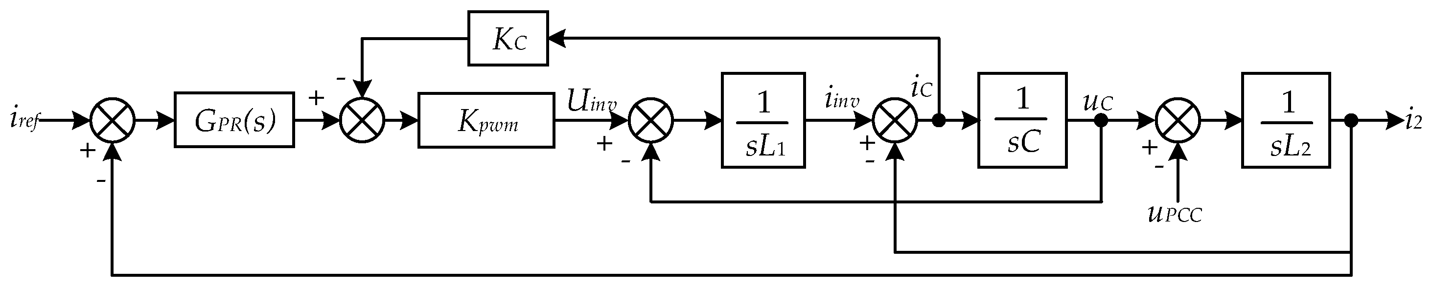
3. Output Impedance Characteristics of the Inverter
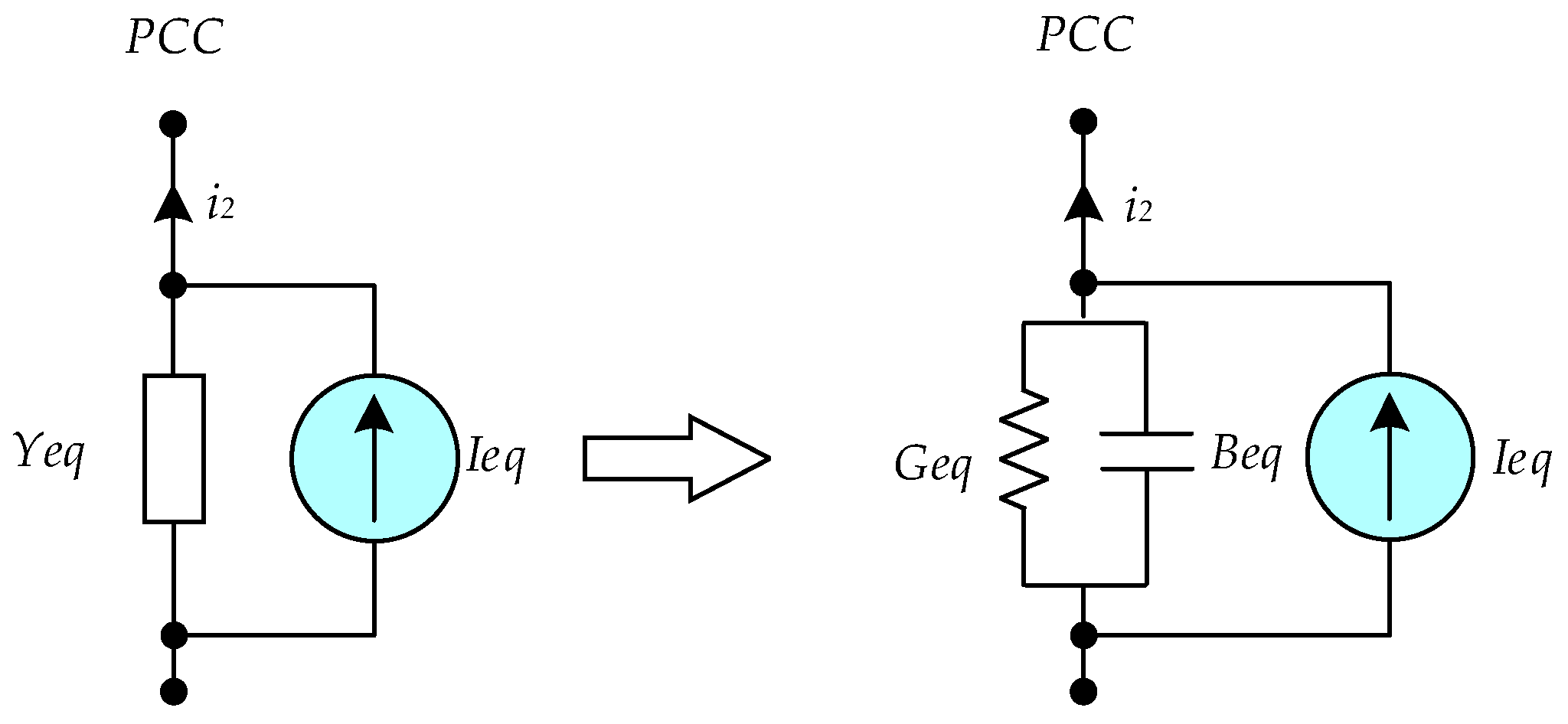
3.1. Equivalent Circuit of the Inverter
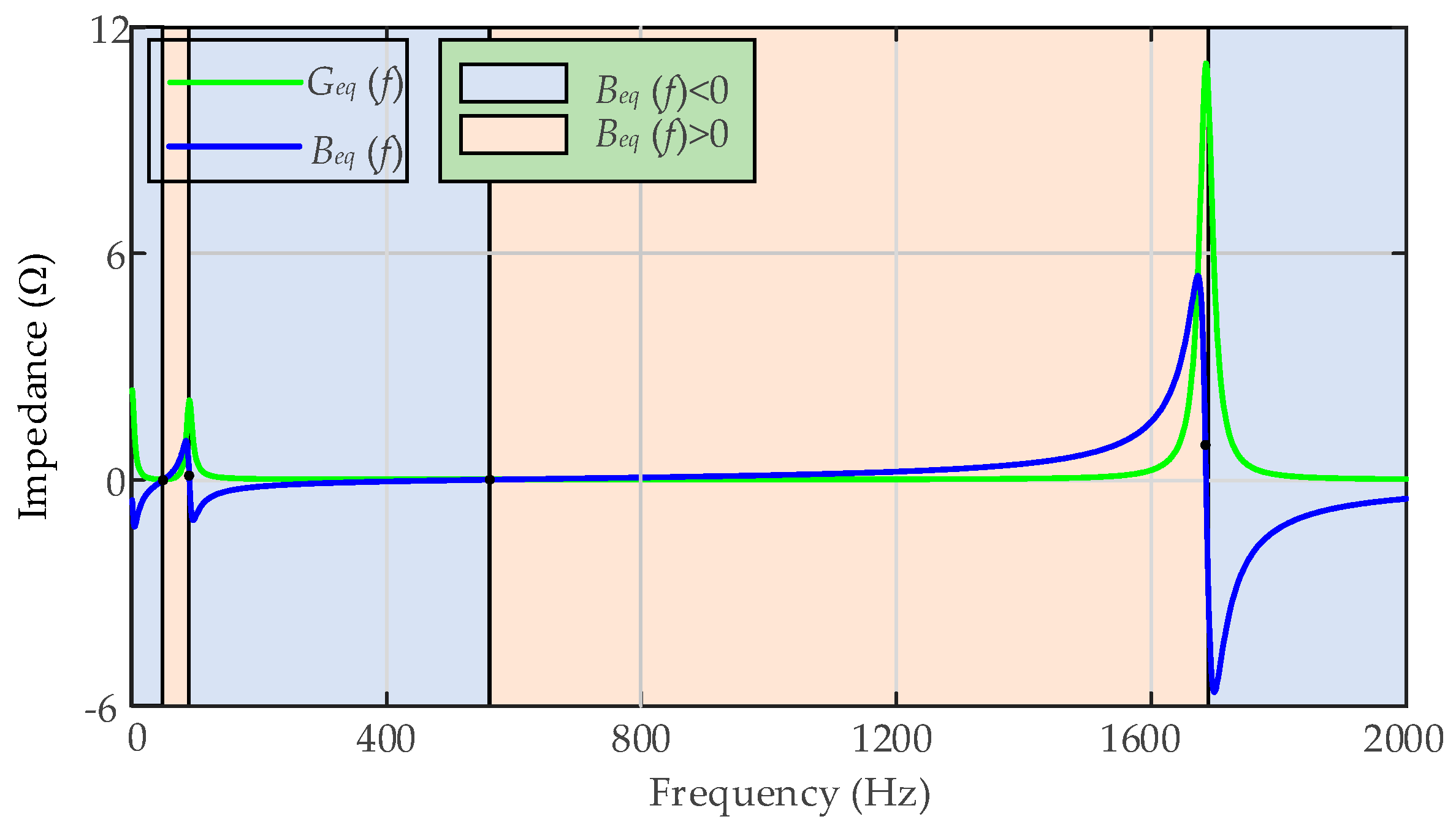
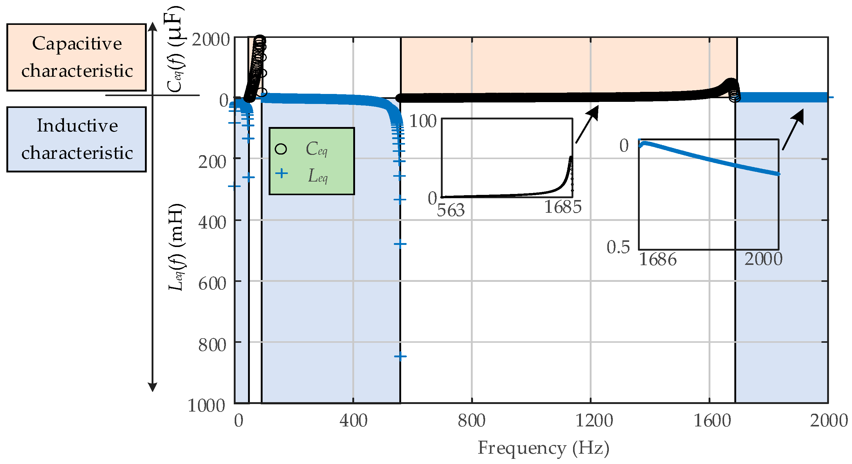
3.2. Output Impedance of the Inverter
3.3. Effect of Grid-Connected Inverter on Impedance Distribution
4. Connection Optimization Scheme of Inverter
4.1. Concept of Security Region
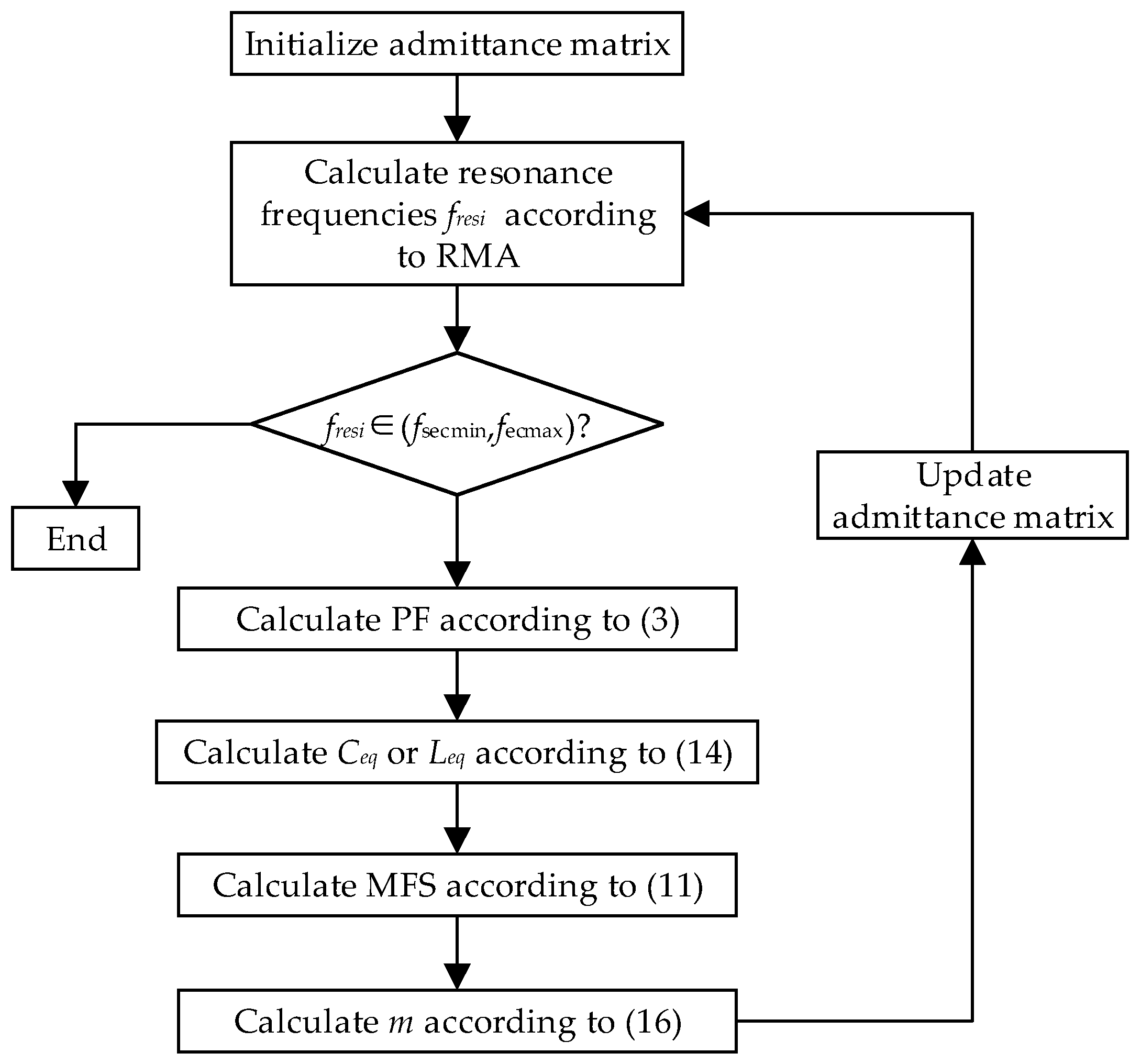
4.2. Study on Optimization Scheme
5. Simulation Verification
6. Discussion
6.1. Optimization Objective
6.2. Improvement of Voltage Quality
6.3. Target Frequency
7. Conclusions
Author Contributions
Funding
Institutional Review Board Statement
Informed Consent Statement
Data Availability Statement
Conflicts of Interest
References
- Liu, B.; Liu, Z.; Liu, J.; An, R.; Zheng, H.; Shi, Y. An Adaptive Virtual Impedance Control Scheme Based on Small-AC-Signal Injection for Unbalanced and Harmonic Power Sharing in Islanded Microgrids. IEEE Trans. Power Electron. 2019, 34, 12333–12355. [Google Scholar] [CrossRef]
- Wei, X.; Li, C.; Qi, M.; Luo, B.; Deng, X.; Zhu, G. Research on Harmonic Current Amplification Effect of Parallel APF Compensating Voltage Source Nonlinear Load. Energies. 2019, 12, 3070. [Google Scholar] [CrossRef] [Green Version]
- Lou, G.; Yang, Q.; Gu, W.; Quan, X.; Guerrero, J.M.; Li, S. Analysis and Design of Hybrid Harmonic Suppression Scheme for VSG Considering Nonlinear Loads and Distorted Grid. IEEE Trans. Energy Convers. 2021, 36, 3096–3107. [Google Scholar] [CrossRef]
- Guerrero-Rodríguez, N.F.; Lucas, L.C.H.; de Pablo-Gómez, S.; Rey-Boué, A.B. Performance study of a synchronization algorithm for a 3-phase photovoltaic grid-connected system under harmonic distortions and unbalances. Electr. Power Syst. Res. 2014, 116, 252–265. [Google Scholar] [CrossRef]
- Smadi, A.A.; Lei, H.; Johnson, K.B. Distribution System Harmonic Mitigation using a PV System with Hybrid Active Filter Features. In Proceedings of the 2019 North American Power Symposium (NAPS), Wichita, KS, USA, 13–15 October 2019; pp. 1–6. [Google Scholar]
- Xiao, X.; Li, Z.; Wang, Y.; Zhou, Y. A Practical Approach to Estimate Harmonic Distortions in Residential Distribution System. IEEE Trans. Power Deliv. 2021, 36, 1418–1427. [Google Scholar] [CrossRef]
- Pereira, J.L.M.; Leal, A.F.R.; Almeida, G.O.D.; Tostes, M.E.D.L. Harmonic Effects Due to the High Penetration of Photovoltaic Generation into a Distribution System. Energies 2021, 14, 4021. [Google Scholar] [CrossRef]
- Guest, E.; Jensen, K.H.; Rasmussen, T.W. Mitigation of Harmonic Voltage Amplification in Offshore Wind Power Plants by Wind Turbines With Embedded Active Filters. IEEE Trans. Sustain. Energy 2020, 11, 785–794. [Google Scholar] [CrossRef]
- Nejabatkhah, F.; Li, Y.W.; Wu, B. Control Strategies of Three-Phase Distributed Generation Inverters for Grid Unbalanced Voltage Compensation. IEEE Trans. Power Electron. 2016, 31, 5228–5241. [Google Scholar]
- Herman, L.; Papič, I. Hybrid active filter for power factor correction and harmonics elimination in industrial networks. In Proceedings of the 2011 IEEE Electrical Power and Energy Conference, Winnipeg, MB, Canada, 3–5 October 2011; pp. 302–308. [Google Scholar]
- Michalec, Ł.; Jasiński, M.; Sikorski, T.; Leonowicz, Z.; Jasiński, Ł.; Suresh, V. Impact of Harmonic Currents of Nonlinear Loads on Power Quality of a Low Voltage Network–Review and Case Study. Energies 2021, 14, 3665. [Google Scholar] [CrossRef]
- Wei, L.; Guskov, N.N.; Lukaszewski, R.A.; Skibinski, G.L. Mitigation of Current Harmonics for Multipulse Diode Front-End Rectifier Systems. IEEE Trans. Ind. Appl. 2007, 43, 787–797. [Google Scholar] [CrossRef]
- Mon-Nzongo, D.L.; Ipoum-Ngome, P.G.; Jin, T.; Song-Manguelle, J. An Improved Topology for Multipulse AC/DC Converters Within HVDC and VFD Systems: Operation in Degraded Modes. IEEE Trans. Power Electron. 2018, 65, 3646–3656. [Google Scholar] [CrossRef]
- Lai, Z.; Smedley, K.M. A family of continuous-conductionmode power-factor-correction controllers based on the general pulse width modulator. IEEE Trans. Power Electron. 1998, 13, 501–510. [Google Scholar]
- Chou, C.-J.; Liu, C.-W.; Lee, J.-Y.; Lee, K.-D. Optimal planning of large passive-harmonic-filters set at high voltage level. IEEE Trans. Power Syst. 2000, 15, 433–441. [Google Scholar] [CrossRef] [Green Version]
- Martinek, R.; Rzidky, J.; Jaros, R.; Bilik, P.; Ladrova, M. Least Mean Squares and Recursive Least Squares Algorithms for Total Harmonic Distortion Reduction Using Shunt Active Power Filter Control. Energies 2019, 12, 1545. [Google Scholar] [CrossRef] [Green Version]
- Zhou, Z.; Li, Y.; Yang, Y.; Huang, X.; Chen, Z. Application of 20 kV high-voltage active power filter (APF). In Proceedings of the 2012 China International Conference on Electricity Distribution, Shanghai, China, 10–14 September 2012; pp. 1–4. [Google Scholar]
- Seifossadat, S.G.; Kianinezhad, R.; Ghasemi, A.; Monadi, M. Quality improvement of shunt active power filter, using optimized tuned harmonic passive filters. In Proceedings of the 2008 International Symposium on Power Electronics, Electrical Drives, Automation and Motion, Ischia, Italy, 11–13 June 2008; pp. 1388–1393. [Google Scholar]
- Wang, X.; Blaabjerg, F.; Loh, P.C. Grid-Current-Feedback Active Damping for LCL Resonance in Grid-Connected Voltage-Source Converters. IEEE Trans. Ind. Electron. 2016, 31, 213–223. [Google Scholar] [CrossRef] [Green Version]
- Li, Z.; Hu, H.; Wang, Y.; Tang, L.; He, Z.; Gao, S. Probabilistic Harmonic Resonance Assessment Considering Power System Uncertainties. IEEE Trans. Power Deliv. 2018, 33, 2989–2998. [Google Scholar] [CrossRef]
- Bouhouras, A.S.; Marinopoulos, A.G.; Labridis, D.P.; Dokopoulos, P.S. Installation of PV systems in Greece—Reliability improvement in the transmission and distribution system. Electr. Power Syst. Res. 2010, 80, 547–555. [Google Scholar] [CrossRef]
- Belenguer, E.; Beltran, H.; Aparicio, N. Distributed generation power inverters as shunt active power filters for losses minimization in the distribution network. In Proceedings of the 2007 European Conference on Power Electronics and Applications, Aalborg, Denmark, 2–5 September 2007; pp. 1–10. [Google Scholar]
- Aghaebrahimi, M.R.; Amiri, M.; Zahiri, S.H. An immune-based optimization method for distributed generation placement in order to minimize power losses. In Proceedings of the 2009 International Conference on Sustainable Power Generation and Supply, Nanjing, China, 6–7 April 2009; pp. 1–6. [Google Scholar]
- Chang, C.; Gorinevsky, D.; Lall, S. Dynamical and Voltage Profile Stability of Inverter-Connected Distributed Power Generation. IEEE Trans. Smart Grid. 2014, 5, 2093–2105. [Google Scholar] [CrossRef]
- Shaheen, A.M.; Elsayed, A.M.; Ginidi, A.R.; El-Sehiemy, R.A.; Elattar, E. A heap-based algorithm with deeper exploitative feature for optimal allocations of distributed generations with feeder reconfiguration in power distribution networks. Knowl.-Based Syst. 2022, 241, 108269. [Google Scholar] [CrossRef]
- Tu, Y.; Liu, J.; Liu, T.; Cheng, X. Impedance-Based Stability Analysis of Large-Scale PV Station under Weak Grid Condition Considering Solar Radiation Fluctuation. In Proceedings of the 2018 International Power Electronics Conference (IPEC-Niigata 2018—ECCE Asia), Niigata, Japan, 20–24 May 2018; pp. 3934–3939. [Google Scholar]
- Teng, J.; Chang, C. Backward/Forward Sweep-Based Harmonic Analysis Method for Distribution Systems. IEEE Trans. Power Deliv. 2007, 22, 1665–1672. [Google Scholar] [CrossRef]
- Xu, W.; Huang, Z.; Cui, Y.; Wang, H. Harmonic resonance mode analysis. IEEE Trans. Power Deliv. 2005, 20, 1182–1190. [Google Scholar] [CrossRef]
- He, Z.; Hu, H.; Zhang, Y.; Gao, S. Harmonic Resonance Assessment to Traction Power-Supply System Considering Train Model in China High-Speed Railway. IEEE Trans. Power Deliv. 2014, 29, 1735–1743. [Google Scholar] [CrossRef]
- Cui, Y.; Wang, X. Modal Frequency Sensitivity for Power System Harmonic Resonance Analysis. IEEE Trans. Power Deliv. 2012, 27, 1010–1017. [Google Scholar] [CrossRef]
- Sauer, P.W.; Pai, M.A. Power System Dynamics and Stability; IEEE Press: New York, NY, USA, 1998; pp. 277–282. [Google Scholar]


| Symbol | Instruction | Values |
|---|---|---|
| Kp | proportionality coefficient | 0.4 |
| Kr | resonance coefficient | 200 |
| ωc | cut-off frequency | 5 |
| Kc | capacitor-current feedback constant | 1 |
| L1 | Inverter-side filter inductor | 4 mH |
| L2 | Grid-side filter inductor | 0.5 mH |
| C | Filter capacitor | 20 μF |
| f0 | Grid frequency | 50 Hz |
| UDC | DC voltage | 700 V |
| Harmonic Source Order h (p.u.) | Bus 5 (A) | Bus 6 (A) | Bus 8 (A) |
|---|---|---|---|
| 5 | 11.2 | 10.3 | 10.0 |
| 7 | 10.6 | 8.5 | 9.0 |
| 11 | 8.6 | 7.3 | 7.5 |
| 13 | 8.9 | 7.1 | 9.2 |
| 17 | 7.0 | 6.8 | 5.7 |
| 19 | 6.4 | 7.1 | 4.5 |
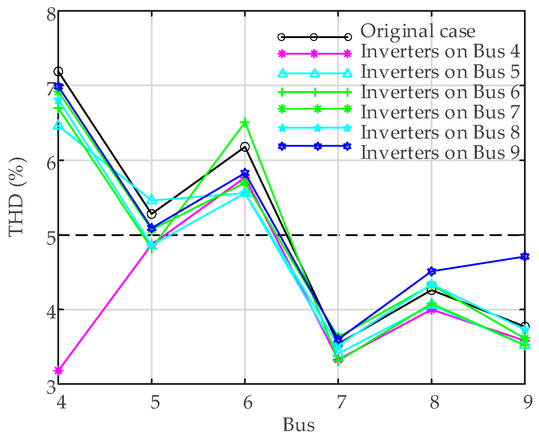
| THD (%) | U4 | U5 | U6 | U7 | U8 | U9 |
|---|---|---|---|---|---|---|
| Original case | 7.19 | 5.28 | 6.18 | 3.54 | 4.26 | 3.77 |
| On Bus 4 | 3.18 | 4.87 | 5.77 | 3.33 | 4.00 | 3.58 |
| On Bus 5 | 6.46 | 5.46 | 5.56 | 3.41 | 4.06 | 3.52 |
| On Bus 6 | 6.7 | 4.82 | 6.51 | 3.31 | 4.08 | 3.52 |
| On Bus 7 | 6.92 | 5.07 | 5.70 | 3.63 | 4.33 | 3.61 |
| On Bus 8 | 6.81 | 4.86 | 5.56 | 3.52 | 4.34 | 3.73 |
| On Bus 9 | 6.99 | 5.09 | 5.83 | 3.60 | 4.51 | 4.71 |
Publisher’s Note: MDPI stays neutral with regard to jurisdictional claims in published maps and institutional affiliations. |
© 2022 by the authors. Licensee MDPI, Basel, Switzerland. This article is an open access article distributed under the terms and conditions of the Creative Commons Attribution (CC BY) license (https://creativecommons.org/licenses/by/4.0/).
Share and Cite
Sun, X.; Lei, W.; Dai, Y.; Yin, Y.; Liu, Q. Optimization Configuration of Grid-Connected Inverters to Suppress Harmonic Amplification in a Microgrid. Energies 2022, 15, 4989. https://doi.org/10.3390/en15144989
Sun X, Lei W, Dai Y, Yin Y, Liu Q. Optimization Configuration of Grid-Connected Inverters to Suppress Harmonic Amplification in a Microgrid. Energies. 2022; 15(14):4989. https://doi.org/10.3390/en15144989
Chicago/Turabian StyleSun, Xing, Wanjun Lei, Yuqi Dai, Yilin Yin, and Qian Liu. 2022. "Optimization Configuration of Grid-Connected Inverters to Suppress Harmonic Amplification in a Microgrid" Energies 15, no. 14: 4989. https://doi.org/10.3390/en15144989
APA StyleSun, X., Lei, W., Dai, Y., Yin, Y., & Liu, Q. (2022). Optimization Configuration of Grid-Connected Inverters to Suppress Harmonic Amplification in a Microgrid. Energies, 15(14), 4989. https://doi.org/10.3390/en15144989