
Flexible Interconnected Distribution Network with Embedded DC System and Its Dynamic Reconfiguration

 ,
,  ,
,
Abstract
:1. Introduction
- (1)
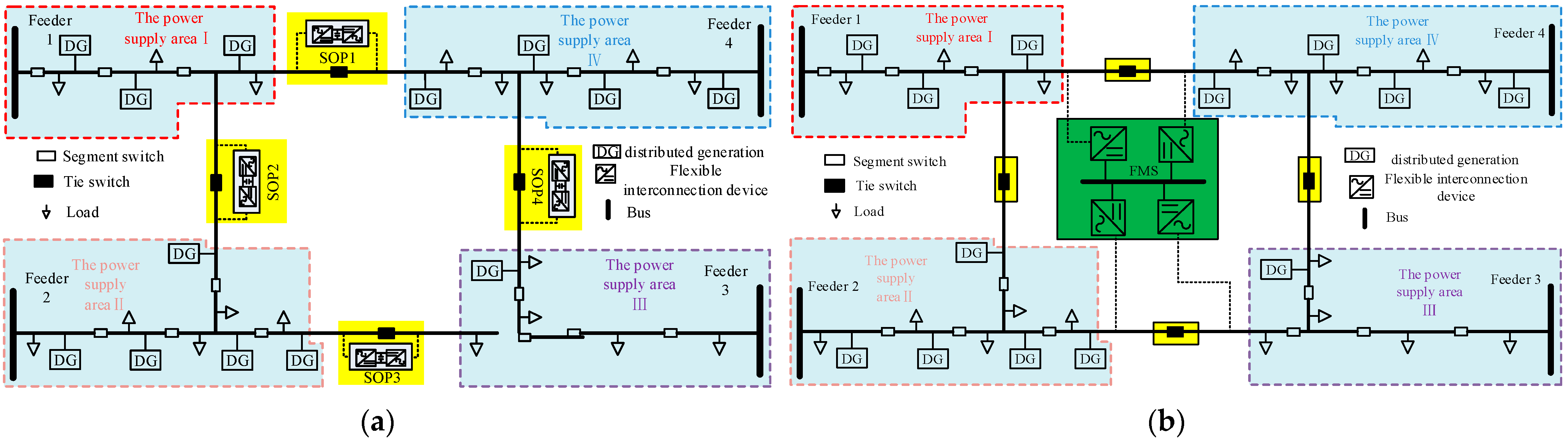
- A new topology of flexible interconnection with better economy is proposed to form a flexible closed loop of the distribution network by EDC, which has high application value in practical application and is suitable for gradual promotion.
- (2)
- A gap is filled in the optimization problem of dynamic reconfiguration of FDN+EDC in the form of complete coexistence of tie switches and FIDs, and a hierarchical coordinated optimization solution method involving an improved particle swarm algorithm is proposed.
2. Flexible Interconnected Distribution Network with Embedded DC System
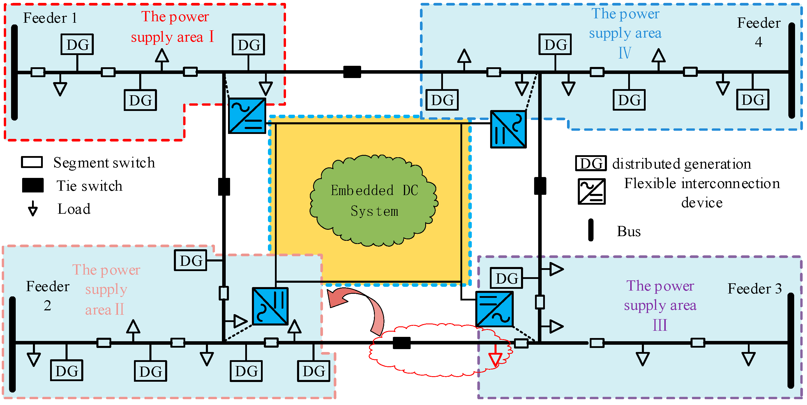
2.1. Topology
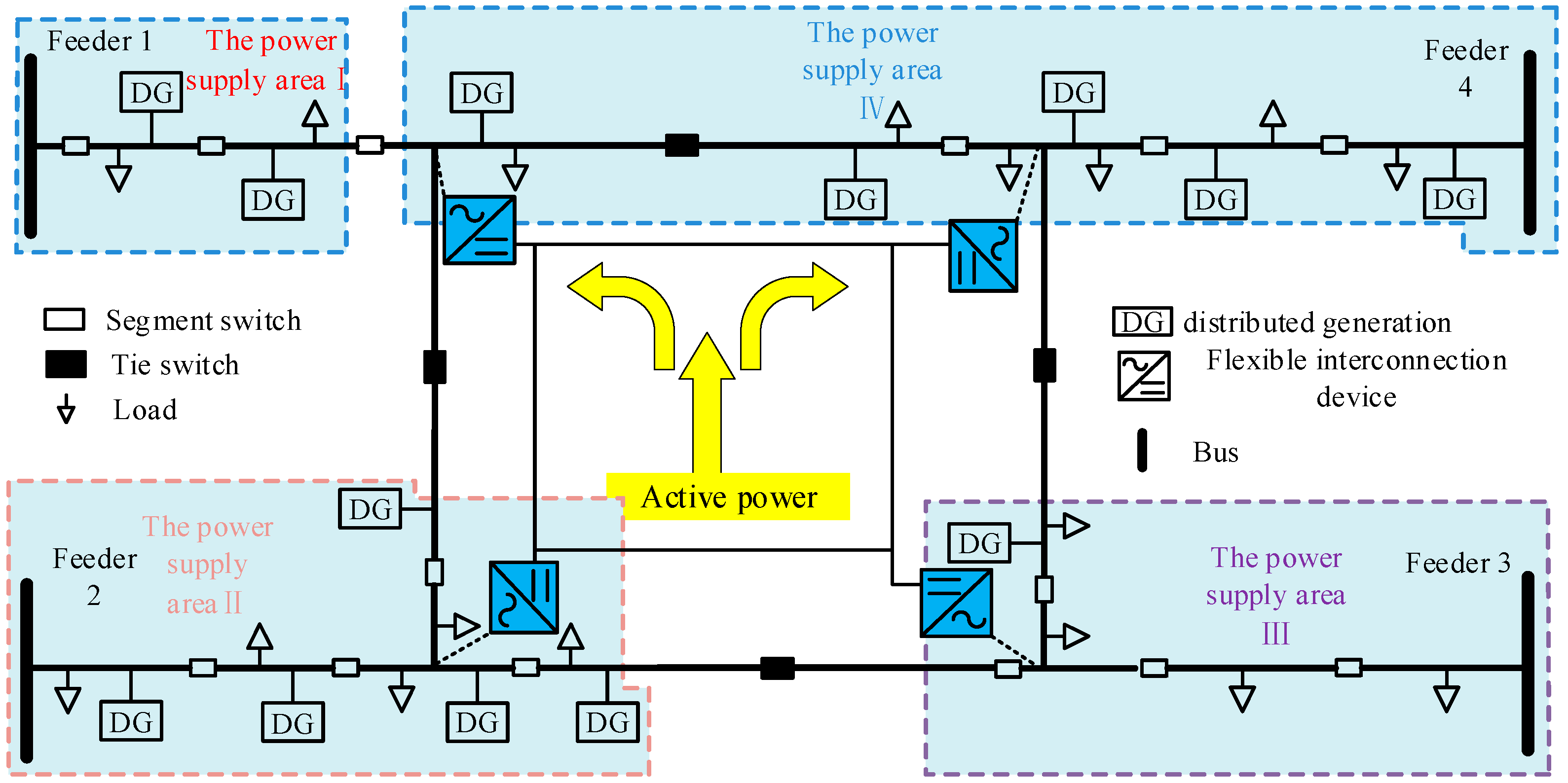
2.2. Operation Mode
3. Dynamic Reconfiguration Optimization Model
3.1. Objective Function
3.2. System Constraints
3.2.1. Power Balance Constraints
- AC side power balance constraint
- DC side power balance constraint
- Power balance at VSCwhere ΔPi(t) and ΔQi(t) are the active and reactive power deviations of AC node i at time t, ΔPdcm(t) is the active power deviation of DC node m at time t, Pgi(t) and Qgi(t) are the active and reactive power of the power supply at AC node i at time t, Pli(t) and Qli(t) are the power of the load, Psi(t) and Qsi(t) are the power flowing through VSC injected into node i at time t. Gij + jBij, θij(t) are the conductance between AC nodes i and j, phase angle at time t, and Pgdcm(t) and Pldcm(t) are the power supply and load power at DC node m at time t. Pcdcm(t) is the active power injected into DC side m by the converter at time t. Gdcmn is the line conductance between DC nodes m, n. Pt,DC·VSCk is the power injected into its DC side portion by the kth VSC at time t.
3.2.2. System Security Operational Constraints
3.2.3. Converter Capacity Constraints
3.2.4. Network Topology Constraints
3.2.5. Switching Action Number Constraints
4. Solution Methodology
4.1. Improved Particle Swarm Algorithm
4.2. Coding of the Problem Solution
4.3. Update of Particles
4.4. Dynamic Reconfiguration Rules
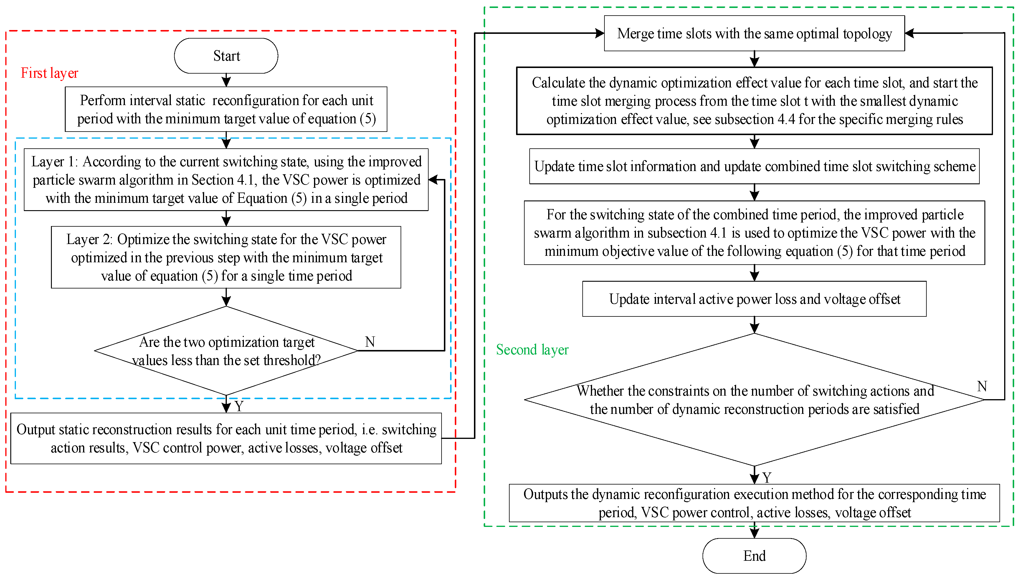
4.5. Dynamic Reconfiguration of Hierarchical Coordination Optimization Methods
5. Case Studies and Analysis
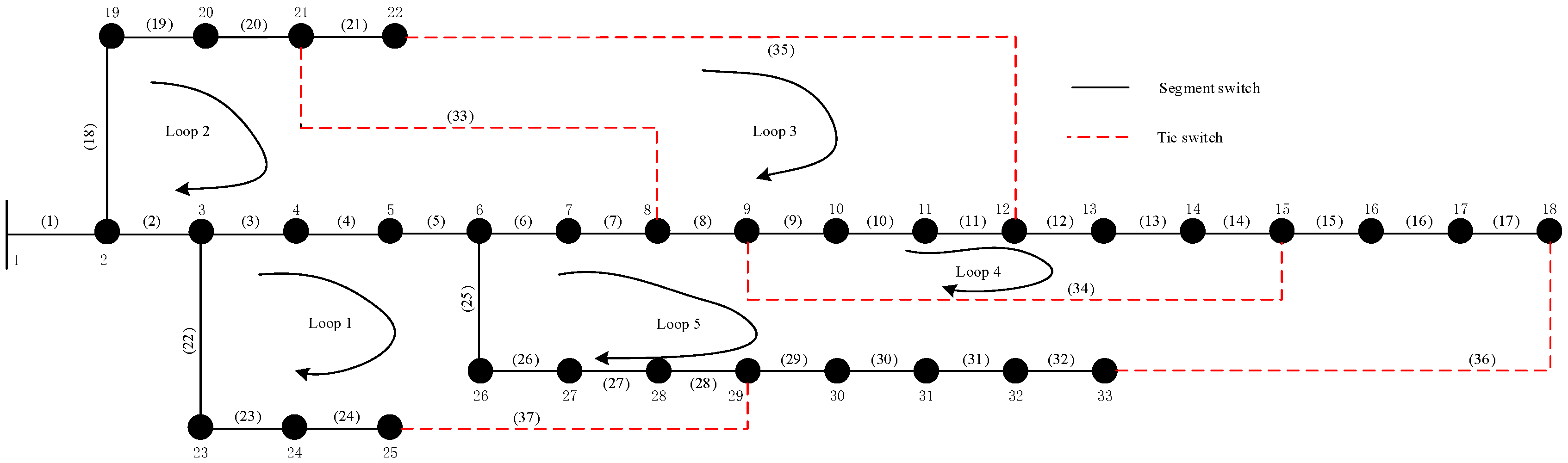
5.1. Network Reconfiguration Analysis of IEEE33-Node System
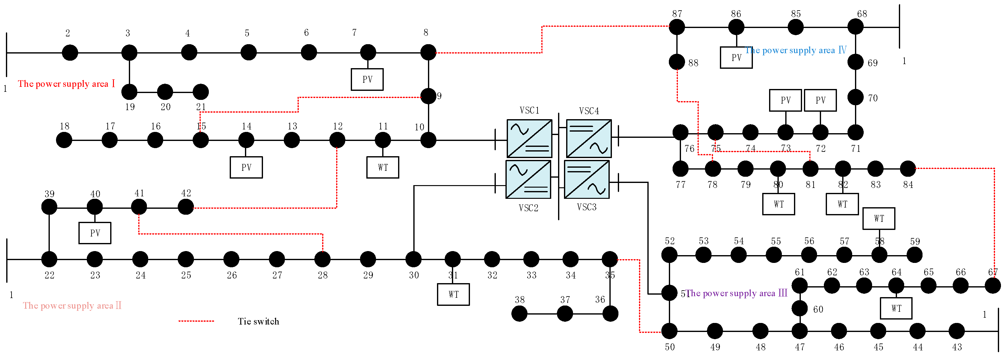
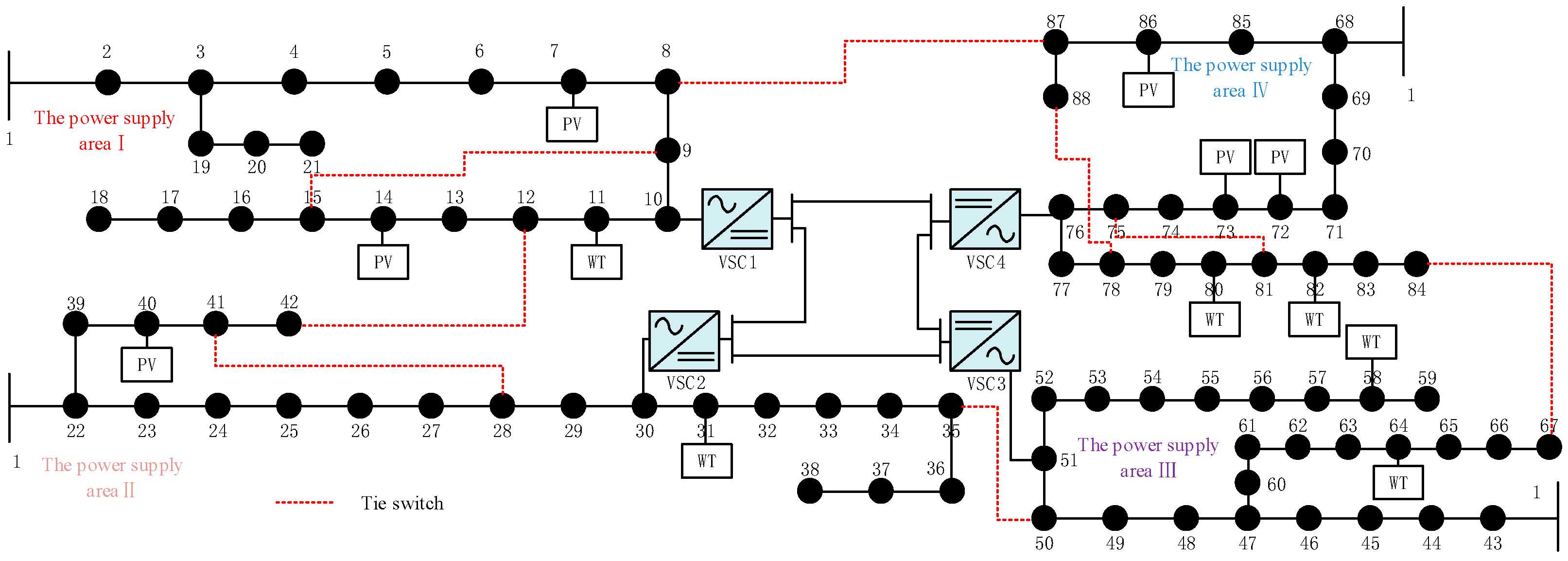
5.2. Modified 88-Node System Based on IEEE 33-Node System
5.3. Comparison of FDN+EDC and FMS Topology
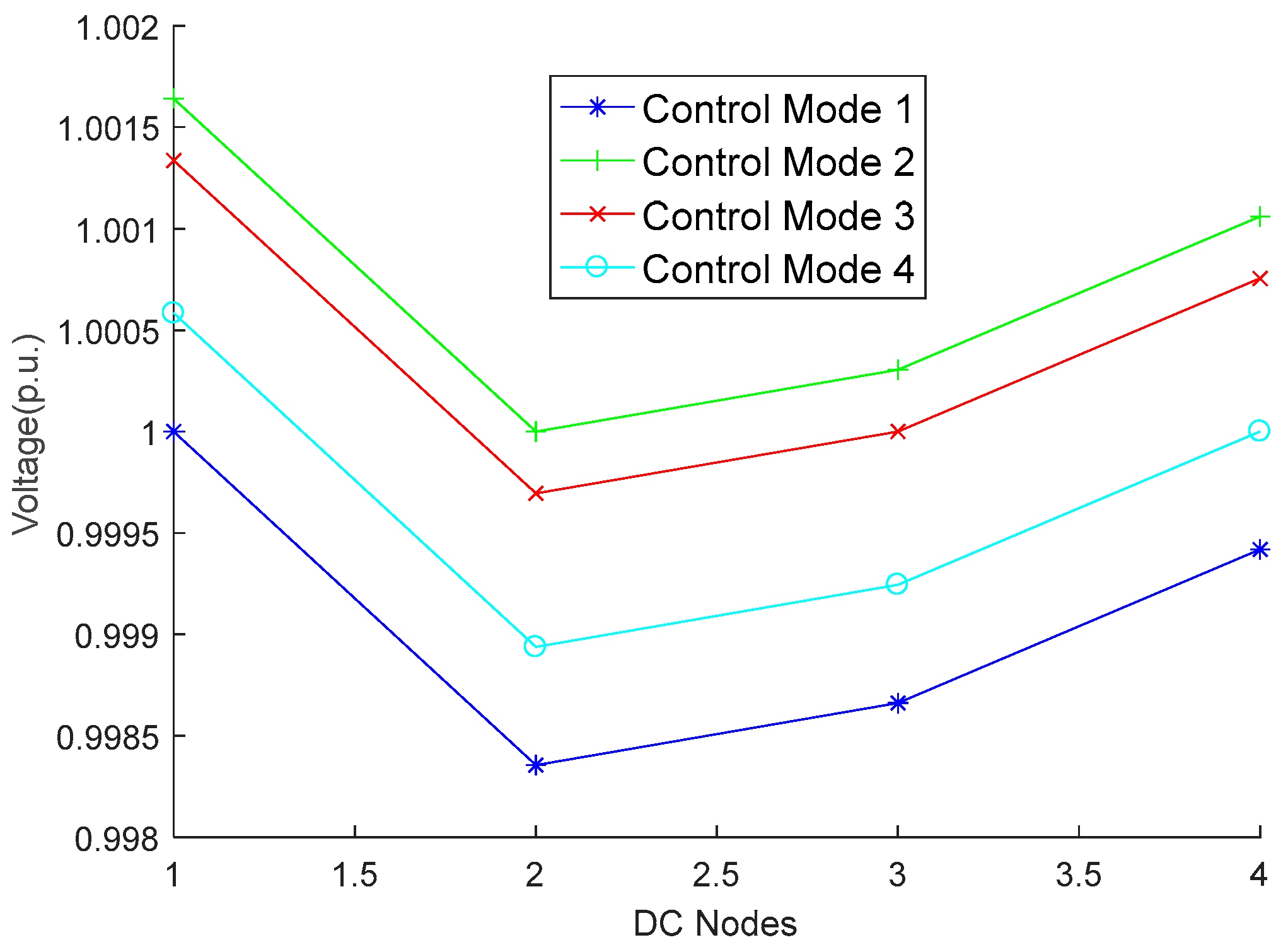
5.4. Influence of Different Control Modes of Each VSC on FDN+EDC
5.5. Impact of VSC Decommissioning on FDN+EDC
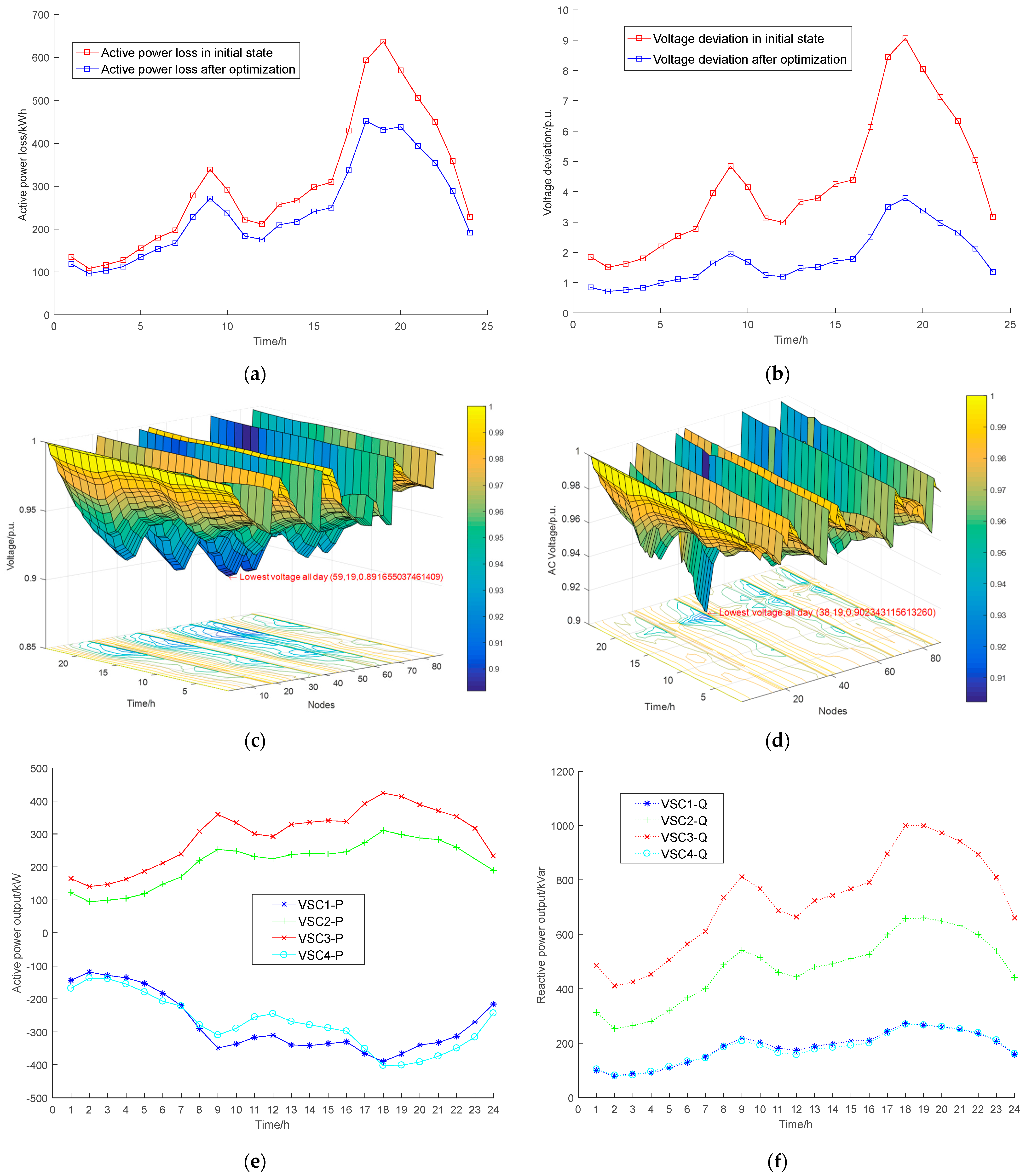
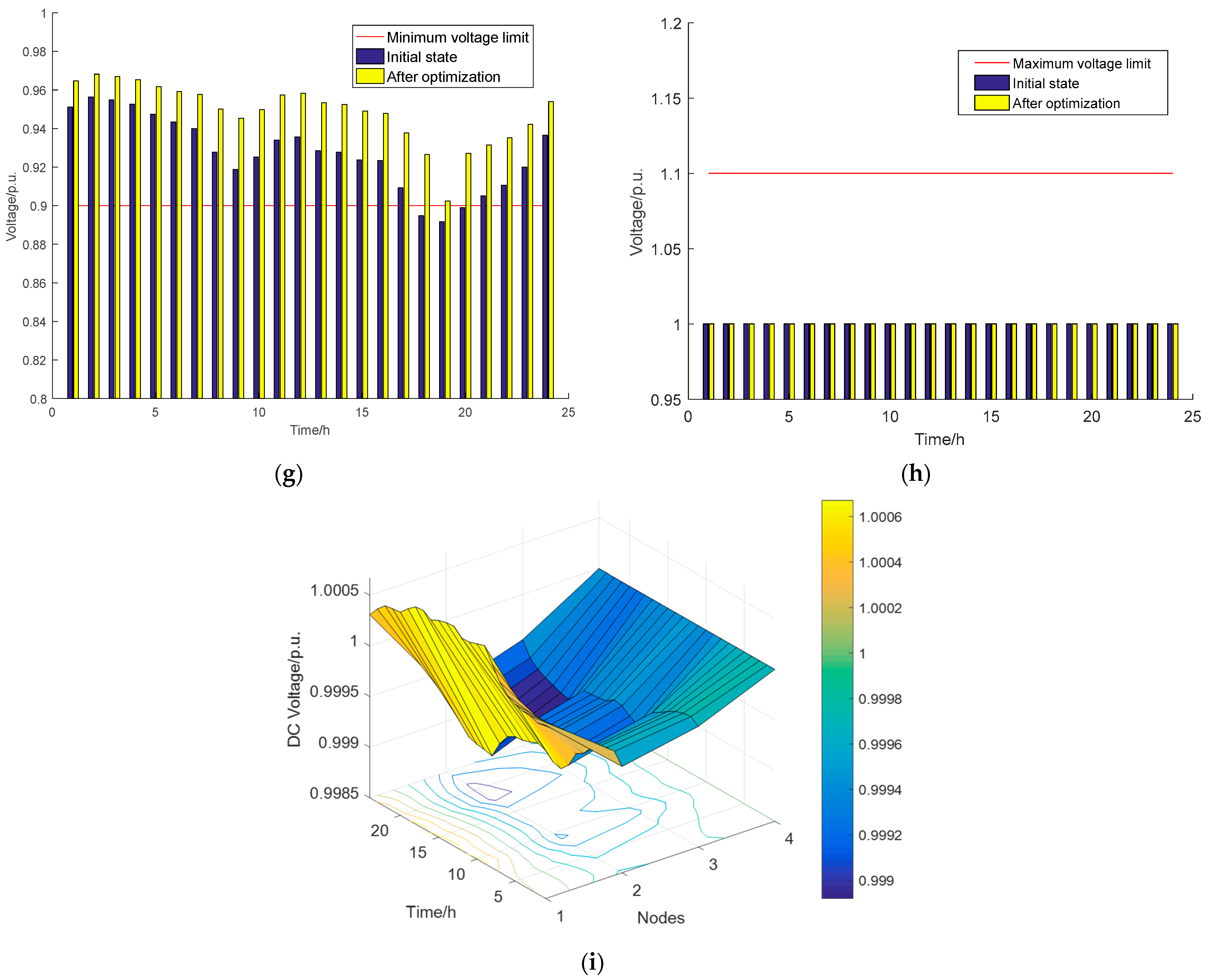
5.6. Dynamic Reconfiguration Optimization
6. Conclusions
Author Contributions
Funding
Institutional Review Board Statement
Informed Consent Statement
Data Availability Statement
Acknowledgments
Conflicts of Interest
References
- Zhu, N.; Jiang, D.; Hu, P.; Yang, Y. Honeycomb Active Distribution Network: A Novel Structure of Distribution Network and Its Stochastic Optimization. In Proceedings of the 2020 15th IEEE Conference on Industrial Electronics and Applications (ICIEA), Kristiansand, Norway, 9–13 November 2020; pp. 455–462. [Google Scholar]
- Qi, Q.; Jiang, Q.R.; Xu, Y.P. Research Status and Development Prospect of Flexible Interconnection for Smart Distribution Networks. Power Syst. Technol. 2020, 44, 4664–4676. (In Chinese) [Google Scholar]
- Ji, H.; Jian, J.; Yu, H.; Ji, J.; Wei, M.; Zhang, X.; Li, P.; Yan, J.; Wang, C. Peer-to-Peer Electricity Trading of Interconnected Flexible Distribution Networks Based on Distributed Ledger. IEEE Trans. Ind. Inform. 2022, 18, 5949–5960. [Google Scholar] [CrossRef]
- Xiao, J.; Wang, Y.; Luo, F.; Bai, L.; Gang, F.; Huang, R.; Jiang, X.; Zhang, X. Flexible distribution network: Definition, configuration, operation, and pilot project. IET Gener. Transm. Distrib. 2018, 12, 4492–4498. [Google Scholar] [CrossRef]
- Zhao, Y.; Xiong, W.; Yuan, X.; Zou, X. A fault recovery strategy of flexible interconnected distribution network with SOP flexible closed-loop operation. Int. J. Electr. Power Energy Syst. 2022, 142, 108360. [Google Scholar] [CrossRef]
- Jiang, X.; Zhou, Y.; Ming, W.; Yang, P.; Wu, J. An Overview of Soft Open Points in Electricity Distribution Networks. IEEE Trans. Smart Grid 2022, 13, 1899–1910. [Google Scholar] [CrossRef]
- Zangiabadi, M.; Tian, Z.; Kamel, T.; Tricoli, P.; Wade, N.; Pickert, V. A Smart Rail and Grid Energy Management System for increased synergy between DC Railway Networks & Electrical Distribution Networks. In Proceedings of the 2021 56th International Universities Power Engineering Conference (UPEC), Middlesbrough, UK, 31 August–3 September 2021; pp. 1–6. [Google Scholar]
- Ji, H.; Wang, C.; Li, P.; Zhao, J.; Song, G.; Wu, J. Quantified flexibility evaluation of soft open points to improve distributed generation penetration in active distribution networks based on difference-of-convex programming. Appl. Energy 2018, 218, 338–348. [Google Scholar] [CrossRef]
- Ji, H.; Wang, C.; Li, P.; Zhao, J.; Song, G.; Ding, F.; Wu, J. An enhanced SOCP-based method for feeder load balancing using the multi-terminal soft open point in active distribution networks. Appl. Energy 2017, 208, 986–995. [Google Scholar] [CrossRef]
- Li, P.; Ji, H.; Wang, C.; Zhao, J.; Song, G.; Ding, F.; Wu, J. Coordinated Control Method of Voltage and Reactive Power for Active Distribution Networks Based on Soft Open Point. IEEE Trans. Sustain. Energy 2017, 8, 1430–1442. [Google Scholar] [CrossRef] [Green Version]
- Shafik, M.B.; Rashed, G.I.; Chen, H. Optimizing Energy Savings and Operation of Active Distribution Networks Utilizing Hybrid Energy Resources and Soft Open Points: Case Study in Sohag, Egypt. IEEE Access 2020, 8, 28704–28717. [Google Scholar] [CrossRef]
- Li, P.; Ji, J.; Ji, H.; Song, G.; Wang, C.; Wu, J. Self-healing oriented supply restoration method based on the coordination of multiple SOPs in active distribution networks. Energy 2020, 195, 116968. [Google Scholar] [CrossRef]
- Liu, W.; Huang, Y.; Yang, Y.; Liu, X. Reliability evaluation and analysis of multi-terminal interconnect power distribution system with flexible multi-state switch. IET Gener. Transm. Distrib. 2020, 14, 4746–4754. [Google Scholar] [CrossRef]
- Su, M.; Huo, Q.; Wei, T.; Guo, X. Flexible Multi-State Switch Application Scenario Analysis. In Proceedings of the 2019 14th IEEE Conference on Industrial Electronics and Applications (ICIEA), Xi’an, China, 19–21 June 2019; pp. 1367–1372. [Google Scholar]
- Cao, W.Y.; Wu, J.Z.; Jenkins, N.; Wang, C.S.; Green, T. Benefits analysis of Soft Open Points for electrical distribution network operation. Appl. Energy 2016, 165, 36–47. [Google Scholar] [CrossRef] [Green Version]
- Khan, M.O.; Wadood, A.; Abid, M.I.; Khurshaid, T.; Rhee, S.B. Minimization of Network Power Losses in the AC-DC Hybrid Distribution Network through Network Reconfiguration Using Soft Open Point. Electronics 2021, 10, 326. [Google Scholar] [CrossRef]
- Qi, Q.; Wu, J.Z. Increasing Distributed Generation Penetration using Network Reconfiguration and Soft Open Points. Energy Procedia 2017, 105, 2169–2174. [Google Scholar] [CrossRef]
- Jian, J.; Li, P.; Yu, H.; Ji, H.R.; Ji, J.; Song, G.Y.; Yan, J.Y.; Wu, J.Z.; Wang, C.S. Multi-stage supply restoration of active distribution networks with SOP integration. Sustain. Energy Grids Netw. 2022, 29, 100562. [Google Scholar] [CrossRef]
- Sun, F.Z.; Ma, J.C.; Yu, M.; Wei, W. Optimized Two-Time Scale Robust Dispatching Method for the Multi-Terminal Soft Open Point in Unbalanced Active Distribution Networks. IEEE Trans. Sustain. Energy 2021, 12, 587–598. [Google Scholar] [CrossRef]
- Cong, P.; Hu, Z.; Tang, W.; Lou, C. Optimal allocation of soft open points in distribution networks based on candidate location opitimization. In Proceedings of the 8th Renewable Power Generation Conference (RPG 2019), Shanghai, China, 24–25 October 2019; pp. 1–6. [Google Scholar]
- Zhang, L.; Shen, C.; Chen, Y.; Huang, S.; Tang, W. Coordinated allocation of distributed generation, capacitor banks and soft open points in active distribution networks considering dispatching results. Appl. Energy 2018, 231, 1122–1131. [Google Scholar] [CrossRef]
- Essallah, S.; Khedher, A. Optimization of distribution system operation by network reconfiguration and DG integration using MPSO algorithm. Renew. Energy Focus 2020, 34, 37–46. [Google Scholar] [CrossRef]
- Clerc, M.; Kennedy, J. The particle swarm-explosion, stability, and convergence in a multidimensional complex space. IEEE Trans. Evol. Comput. 2002, 6, 58–73. [Google Scholar] [CrossRef] [Green Version]
- Salau, A.O.; Gebru, Y.W.; Bitew, D. Optimal network reconfiguration for power loss minimization and voltage profile enhancement in distribution systems. Heliyon 2020, 6, e04233. [Google Scholar] [CrossRef]
- Zhu, J.Z. Optimal reconfiguration of electrical distribution network using the refined genetic algorithm. Electr. Power Syst. Res. 2002, 62, 37–42. [Google Scholar] [CrossRef]


| Method | Disconnect Switch | Best Loss/kW | Worst Loss/kW | Average Loss/kW | Standard Deviation/kW | Average Loss Reduction (%) | Loss Reduction (Best Value) (%) | Minimum Voltage (p.u.) |
|---|---|---|---|---|---|---|---|---|
| RGA [25] | 7, 9, 14, 37, 32 | 139.5 | 198.4 | 164.9 | 13.34 | 18.65 | 31.2 | 0.9315 |
| This paper | 7, 9, 14, 37, 32 | 139.551 | 140.279 | 139.557 | 0.05937 | 31.143 | 31.146 | 0.9378 |
| Topology | Line | r (p.u.) | x (p.u.) |
|---|---|---|---|
| FMS | 10-VSC1 | 1.247851 | 1.247851 |
| 30-VSC2 | 1.247851 | 1.247851 | |
| 51-VSC3 | 0.779907 | 0.779907 | |
| 76-VSC4 | 0.779907 | 0.779907 | |
| FDN+EDC | VSC1-VSC2 | 1.247851 | - |
| VSC1-VSC4 | 1.247851 | - | |
| VSC2-VSC3 | 1.247851 | - | |
| VSC3-VSC4 | 0.311963 | - |
| Topology | Disconnect Switch | VSC1P/ kW | VSC2P/ kW | VSC3P/ kW | VSC4P/ kW | VSC1Q/ kVar | VSC2Q/ kVar | VSC3Q/ kVar | VSC4Q/ kVar | Active Loss/MW | Voltage Offset |
|---|---|---|---|---|---|---|---|---|---|---|---|
| Initial state | 8-87/9-15/12-42/28-41/35-50/67-84/75-81/78-88 | — | — | — | — | — | — | — | — | 0.637 | 9.060 |
| FMS | 8-87/9-15/12-42/28-41/35-50/67-84/75-81/78-88 | −68.097 | 18.791 | 224.710 | −215.711 | 346.754 | 400.689 | 813.069 | 357.234 | 0.588 | 6.561 |
| FMS+Switch | 9-10/14-15/28-41/35-50/75-76/80-81/65-66/8-87 | −290.329 | 235.567 | 354.077 | −342.820 | 195.6328 | 481.215 | 810.314 | 215.790 | 0.4958 | 4.306 |
| FDN+EDC | 10-11/14-15/26-27/35-50/68-69/76-77/63-64/8-87 | −366.655 | 298.162 | 413.692 | −400.885 | 266.3808 | 660.084 | 999.284 | 267.124 | 0.432 | 3.797 |
| Topology | Disconnect Switch | VSC1P/ kW | VSC2P/ kW | VSC3P/ kW | VSC4P/ kW | VSC1Q/ kVar | VSC2Q/ kVar | VSC3Q/ kVar | VSC4Q/ kVar | Active Loss/MW | Voltage Offset |
|---|---|---|---|---|---|---|---|---|---|---|---|
| Initial state | 8-87/9-15/12-42/28-41/35-50/67-84/75-81/78-88 | — | — | — | — | — | — | — | — | 0.637 | 9.060 |
| FMS | 8-87/9-15/12-42/28-41/35-50/67-84/75-81/78-88 | −61.223 | 19.079 | 203.823 | −197.939 | 303.814 | 355.012 | 747.868 | 315.587 | 0.587 | 6.769 |
| FDN+EDC | 8-87/9-15/12-42/28-41/35-50/67-84/75-81/78-88 | −78.122 | 24.721 | 242.538 | −236.438 | 428.468 | 499.800 | 931.663 | 395.398 | 0.574 | 6.180 |
| Control Mode | VSC1 | VSC2 | VSC3 | VSC4 | Disconnect Switch | VSC1P | VSC2P | VSC3P | VSC4P | VSC1Q | VSC2Q | VSC3Q | VSC4Q | Active Loss/MW | Voltage Offset |
|---|---|---|---|---|---|---|---|---|---|---|---|---|---|---|---|
| 1 | UdcQ | PQ | PQ | PQ | 9-10/14-15/ 28-41/35-50/75-76/80-81/65-66/8-87 | −366.046 | 297.856 | 413.900 | −401.326 | 264.108 | 658.670 | 998.300 | 267.653 | 0.483 | 3.833 |
| 2 | PQ | UdcQ | PQ | PQ | 9-10/14-15/ 28-41/35-50/75-76/80-81/65-66/8-87 | −366.010 | 297.483 | 413.414 | −400.437 | 265.748 | 659.316 | 999.405 | 267.330 | 0.483 | 3.832 |
| 3 | PQ | PQ | UdcQ | PQ | 9-10/14-15/ 28-41/35-50/75-76/80-81/65-66/8-87 | −365.674 | 297.293 | 413.156 | −400.426 | 266.659 | 659.260 | 1000.395 | 266.734 | 0.483 | 3.832 |
| 4 | PQ | PQ | PQ | UdcQ | 10-11/14-15/26-27/35-50/68-69/76-77/63-64/8-87 | −366.655 | 298.162 | 413.692 | −400.885 | 266.381 | 660.084 | 999.284 | 267.124 | 0.432 | 3.797 |
| Number of Returns | Returned VSC | Disconnect Switch | VSC1P | VSC2P | VSC3P | VSC4P | VSC1Q | VSC2Q | VSC3Q | VSC4Q | Active Loss/MW | Voltage Offset |
|---|---|---|---|---|---|---|---|---|---|---|---|---|
| 1 | VSC1 | 9-10/14-15/28-41/35-50/75-76/80-81/65-66/8-87 | — | 184.191 | 302.564 | −534.189 | — | 663.686 | 1002.005 | 300.9895 | 0.490 | 4.095 |
| VSC2 | 11-12/14-15/28-41/34-35/75-76/80-81/65-66/8-87 | −204.555 | — | 680.66 | −523.864 | 303.370 | — | 1201.313 | 299.5803 | 0.488 | 3.924 | |
| VSC3 | 9-10/14-15/28-41/35-50/75-76/80-81/65-66/8-87 | −339.843 | 328.136 | — | −19.1796 | 259.685 | 664.356 | — | 350.4404 | 0.524 | 5.489 | |
| VSC4 | 11-12/14-15/28-41/34-35/75-76/80-81/65-66/8-87 | −319.602 | −272.265 | 544.745 | — | 336.784 | 445.879 | 1193.51 | — | 0.495 | 4.103 | |
| 2 | VSC1/VSC2 | 11-12/14-15/28-41/34-35/75-76/80-81/65-66/8-87 | — | — | 593.87 | −635.765 | — | — | 1214.539 | 327.172 | 0.492 | 4.096 |
| VSC1/VSC3 | 9-10/14-15/28-41/35-50/75-76/80-81/65-66/8-87 | — | 334.913 | — | −359.775 | — | 690.991 | — | 263.0188 | 0.522 | 5.570 | |
| VSC1/VSC4 | 11-12/14-15/28-41/34-35/75-76/80-81/65-66/8-87 | — | −437.071 | 397.586 | — | — | 497.469 | 1209.586 | — | 0.503 | 4.387 | |
| VSC2/VSC3 | 9-10/14-15/28-41/35-50/75-76/80-81/65-66/8-87 | −148.5 | — | — | 135.058 | 213.683 | — | — | 384.489 | 0.541 | 6.390 | |
| VSC2/VSC4 | 9-10/14-15/28-41/35-50/75-76/80-81/65-66/8-87 | −605.275 | — | 562.987 | — | 335.331 | — | 1214.356 | — | 0.491 | 4.073 | |
| VSC3/VSC4 | 9-10/14-15/28-41/35-50/75-76/80-81/65-66/8-87 | −354.728 | 330.03 | — | — | 271.371 | 687.427 | — | — | 0.523 | 5.575 | |
| 3 | VSC1,2,3 | 9-10/14-15/28-41/35-50/75-76/80-81/65-66/8-87 | — | — | — | −2.997 | — | — | — | 149.8518 | 0.540 | 6.603 |
| VSC1,2,4 | 9-10/14-15/28-41/35-50/75-76/80-81/65-66/8-87 | — | — | −21.411 | — | — | — | 1070.322 | — | 0.515 | 5.330 | |
| VSC1,3,4 | 9-10/14-15/28-41/35-50/75-76/80-81/65-66/8-87 | — | −14.275 | — | — | — | 713.609 | — | — | 0.532 | 5.925 | |
| VSC2,3,4 | 9-10/14-15/28-41/35-50/75-76/80-81/65-66/8-87 | −3.528 | — | — | — | 176.4 | — | — | — | 0.540 | 6.592 |
| Scenario | Disconnect Switch | Switch off Period | Active Power Loss of the Whole Network (kWh) | Voltage Offset of the Whole Network |
|---|---|---|---|---|
| Initial state | 8-87/9-15/12-42/28-41/35-50/67-84/75-81/78-88 | 1–24 h | 7263.7789 | 102.802 |
| After optimization | 9-10/14-15/28-41/35-50/75-76/80-81/65-66/8-87 | 1–18 h | 5783.1496 | 42.91078 |
| 10-11/14-15/26-27/35-50/68-69/76-77/63-64/8-87 | 19 h | |||
| 9-10/14-15/28-41/35-50/75-76/80-81/65-66/8-87 | 20–24 h |
Publisher’s Note: MDPI stays neutral with regard to jurisdictional claims in published maps and institutional affiliations. |
© 2022 by the authors. Licensee MDPI, Basel, Switzerland. This article is an open access article distributed under the terms and conditions of the Creative Commons Attribution (CC BY) license (https://creativecommons.org/licenses/by/4.0/).
Share and Cite
Cai, H.; Yuan, X.; Xiong, W.; Zheng, H.; Xu, Y.; Cai, Y.; Zhong, J. Flexible Interconnected Distribution Network with Embedded DC System and Its Dynamic Reconfiguration. Energies 2022, 15, 5589. https://doi.org/10.3390/en15155589
Cai H, Yuan X, Xiong W, Zheng H, Xu Y, Cai Y, Zhong J. Flexible Interconnected Distribution Network with Embedded DC System and Its Dynamic Reconfiguration. Energies. 2022; 15(15):5589. https://doi.org/10.3390/en15155589
Chicago/Turabian StyleCai, Huan, Xufeng Yuan, Wei Xiong, Huajun Zheng, Yutao Xu, Yongxiang Cai, and Jiumu Zhong. 2022. "Flexible Interconnected Distribution Network with Embedded DC System and Its Dynamic Reconfiguration" Energies 15, no. 15: 5589. https://doi.org/10.3390/en15155589
APA StyleCai, H., Yuan, X., Xiong, W., Zheng, H., Xu, Y., Cai, Y., & Zhong, J. (2022). Flexible Interconnected Distribution Network with Embedded DC System and Its Dynamic Reconfiguration. Energies, 15(15), 5589. https://doi.org/10.3390/en15155589