Modified Particle Swarm Optimization with Attention-Based LSTM for Wind Power Prediction

Abstract

The accuracy of wind power prediction is crucial for the economic operation of a wind power dispatching management system. Wind power generation is closely related to the meteorological conditions around wind plants; a small variation in wind speed could lead to a large fluctuation in the extracted power and is difficult to predict accurately, causing difficulties in grid connection and generating large economic losses. In this study, a wind power prediction model based on a long short-term memory network with a two-stage attention mechanism is established. An attention mechanism is used to measure the input data characteristics and trend characteristics of the wind power and reduce the initial data preparation process. The model effectively alleviates the intermittence and fluctuation of meteorological conditions and improves prediction accuracy significantly. In addition, the modified particle swarm optimization algorithm is introduced to optimize the hyperparameters of the LSTM network, which speeds up the convergence of the model dramatically and avoids falling into local optima, reducing the influence of man-made random selection of LSTM network hyperparameters on the prediction results. The simulation results on the real wind power data show that the modified model has increased prediction accuracy compared with the previous machine learning methods. The monitoring and data collecting system for wind farms reveals that the accuracy of the model is around 95.82%.

1. Introduction

With the continuous consumption of fossil fuels in the electric power industry, the environmental pollution caused by burning fossil fuels is becoming more and more serious [1]. The proportion of thermal power generation in the world is gradually decreasing. Clean energy such as wind, solar and tidal energy has been developing quickly [2]. Wind energy supply in most countries is abundant and inexhaustible, and wind energy conversion technology is relatively simple, so it is included in the key considerations of many countries. Wind energy’s extreme volatility, intermittency, and randomness may cause power fluctuations and have an impact on the regional grid’s overall operation [3]. As a result, when wind farms, particularly high-capacity wind farms, are connected to the grid, they introduce some hidden dangers to the overall power system’s safety and stability [4]. These variable, intermittent, and random characteristics will have a significant impact on wind turbine power’s generating efficiency and service life. As a possible solution to the aforementioned issues, a power dispatching management system requires an effective wind power forecast method in order to design a reasonable power generating plan and improve the grid’s economy, safety, and reliability [5,6,7].

The problem of wind power prediction has attracted a lot of attention from researchers in related fields. Recently released wind power prediction methods can be divided into three categories: physical, statistical, and machine learning methods from the methodological point of view.

The physical method uses a numerical weather forecast produced by a meteorological service to mimic the weather in the wind farm area. The weather data, physical facts surrounding the wind turbine, and the height of the wind turbine’s hub center are then combined to construct a prediction model. Finally, the forecasted power is determined using the wind turbine’s power curve [8]. However, physical methods are greatly limited in wind power prediction and have poor prediction accuracy due to the limitations of complex mathematical calculations and the difficulty of accurately modeling environmental factors.

Statistical methods are adopted to fit complex functional relationships between historical data, weather forecasting data, and forecasting results through one or more mathematical tools. They are basically used to find mathematical patterns in a large amount of data and to adjust forecasting based on the patterns found from this data. Statistical models mainly include autoregressive models, autoregressive sliding average models, and integrated sliding average autoregressive models. However, wind power series data are highly stochastic and intermittent, making their data very complex, and these statistical models cannot extract the corresponding nonlinear features well [9], so there is still much room for improvement in statistical prediction methods.

With the fast growth of deep learning in recent years, machine learning has been extensively used to load prediction. Methods for machine learning primarily include genetic algorithms, artificial neural networks, fuzzy logic, support vector machines, etc. [10]. Since neural networks may potentially infinitely approximate any linear or nonlinear connection, they are frequently employed to tackle classification and regression issues. However, artificial neural networks have intrinsic disadvantages: they are computationally demanding, susceptible to local optima, and sensitive to starting parameters, among others. To circumvent these disadvantages, researchers have developed interval prediction of wind power generation based on particle swarm optimization back propagation neural networks [11]. With the fast development of deep learning methods in the disciplines of image and natural language processing, many researchers have attempted to use these techniques to address other issues. The literature [12] employs a single LSTM for predicting the operational state of a transformer. It considerably enhances the accuracy of predictions. For wind power prediction, the literature [13] blends long short-term memory (LSTM) and attention techniques. In addition, deep learning models were utilized in the literature [14] for energy power forecasting. The literature [15] used PSO-LSTM for the short-term prediction of non-time-series electricity price signals and optimized the LSTM network input weights using particle swarm techniques. However, the effects of the particle swarm’s own weights and learning rate on the global optimal solution were not considered. In addition, in recent years, some improved advanced algorithms have been proposed for load forecasting [16,17,18,19,20], and we will be showing a comparison between available and proposed technology and highlighting the novelty and advantages of these in

Table 1. Model comparison.

Model Name	Novelty and Advantage	Deficiency
Modified-LSTM [16]	Hybrid model is proposed for classification and prediction	Not compared with advanced algorithms
GA-PSO-ANN [17]	Using optimization algorithm to adjust neural network parameters	No optimization for neural network hyperparameters
Multi-Sequence LSTM-RNN [18]	Proposed multi-sequence deep learning model based on meta heuristic algorithm	Lack of data processing and feature extraction
MFF-SAM-GCN [19]	It can effectively capture external features that have an impact on load forecasting	The relationship between weather factors is not analyzed and extracted
CEEMD-WOA-ELMAN [20]	A new meta-heuristic algorithm WOA is introduced to optimize the model	There is a large error between different time scales
MPSO_ATT_LSTM	The features between data are extracted and the hyperparameters of neural network are optimized	Discuss in part of conclusion

.

Wind power generation is highly dependent on meteorological variables such as wind velocity. Traditional forecasting techniques, such as analyzing the impacts of variables on wind power generation using Pearson correlation coefficients, increase the model’s complexity. Inspired by the attention mechanism for letter alignment in the field of natural language translation [21], we built an attention mechanism model that enables the model to learn multiple weights for input data. In this research, an LSTM model with a two-stage attention mechanism is developed for forecasting wind power generation using the time series of wind power generation and relevant meteorological variables. Two components comprise the model: an encoder and a decoder. Based on the LSTM structure, the attention mechanism weights are learned for the input weather data during the encoding stage. A similar daily attention approach based on time windows is presented for the decoding step by comparing the encoder’s output at each moment. Meanwhile, LSTM networks usually use the Adam optimizer for the parameter optimization of neural networks, but the hyperparameters of the network are set by humans, and the setting of hyperparameters has a large impact on the fitting results of the model. Therefore, we will introduce the MPSO algorithm to perform the hyperparameter search for LSTM networks. Finally, we input all the information into the MPSO_ATT_LSTM model proposed in this paper to predict wind power. This paper is structured as follows: Section 2 introduces particle swarm optimization (PSO) and proposes modified particle swarm optimization (MPSO). Section 3 introduces the LSTM model with a two-stage attention mechanism. Section 4 introduces the fused MPSO_ATT_LSTM model. Simulation experiments are conducted in Section 5, and the results are quantitatively analyzed. The conclusion and outlook are presented in Section 6.

2. Optimization Algorithm

2.1. Particle Swarm Optimization (PSO)

Particle swarm optimization (PSO) was derived from the study of bird predation behavior. The basic idea of PSO is to find the global optimal solution by sharing information among individuals in the population [22]. Each particle in the algorithm can be regarded as a possible optimal solution, the individual information of each particle is defined in terms of position and velocity, and finally, the optimization result is described by the fitness value. The particles iterate continuously, both to complete the global search for the optimal solution in the search space and finally to obtain the optimal solution that satisfies the termination condition or reaches the maximum of iterations [23]. In the search space, multiple particles form a population, and the velocity and position of the particles are formed after the $t$ iteration, represented by $V_{i,t}$ and $X_{i,t}$. In the search process, the particles continuously update their positions and velocities and finally obtain the individual extremes $P_{best,i}$ and the global optimal solution $g_{best,i}$ [24,25,26]. The particles update their velocity and position according to Equations (4) and (5):

$$\begin{array}{c}{V}_{i,t+1}=\omega V_{i,t}+c_1 \mathrm{rand} \left(p_{\mathrm{best} }-X_{i,t}\right)+c_2 \mathrm{rand} \left(g_{\mathrm{best} }-X_{i,t}\right)\end{array}$$

(1)

$$\begin{array}{c}{X}_{i,t+1}=X_{i,t}+\lambda V_{i,t+1}\end{array}$$

(2)

where c₁, c₂ are the learning factors of individual particles and population; ω is the inertia weight; rand is a random number between [0, 1]; and λ is the velocity coefficient, which is generally set to 1.

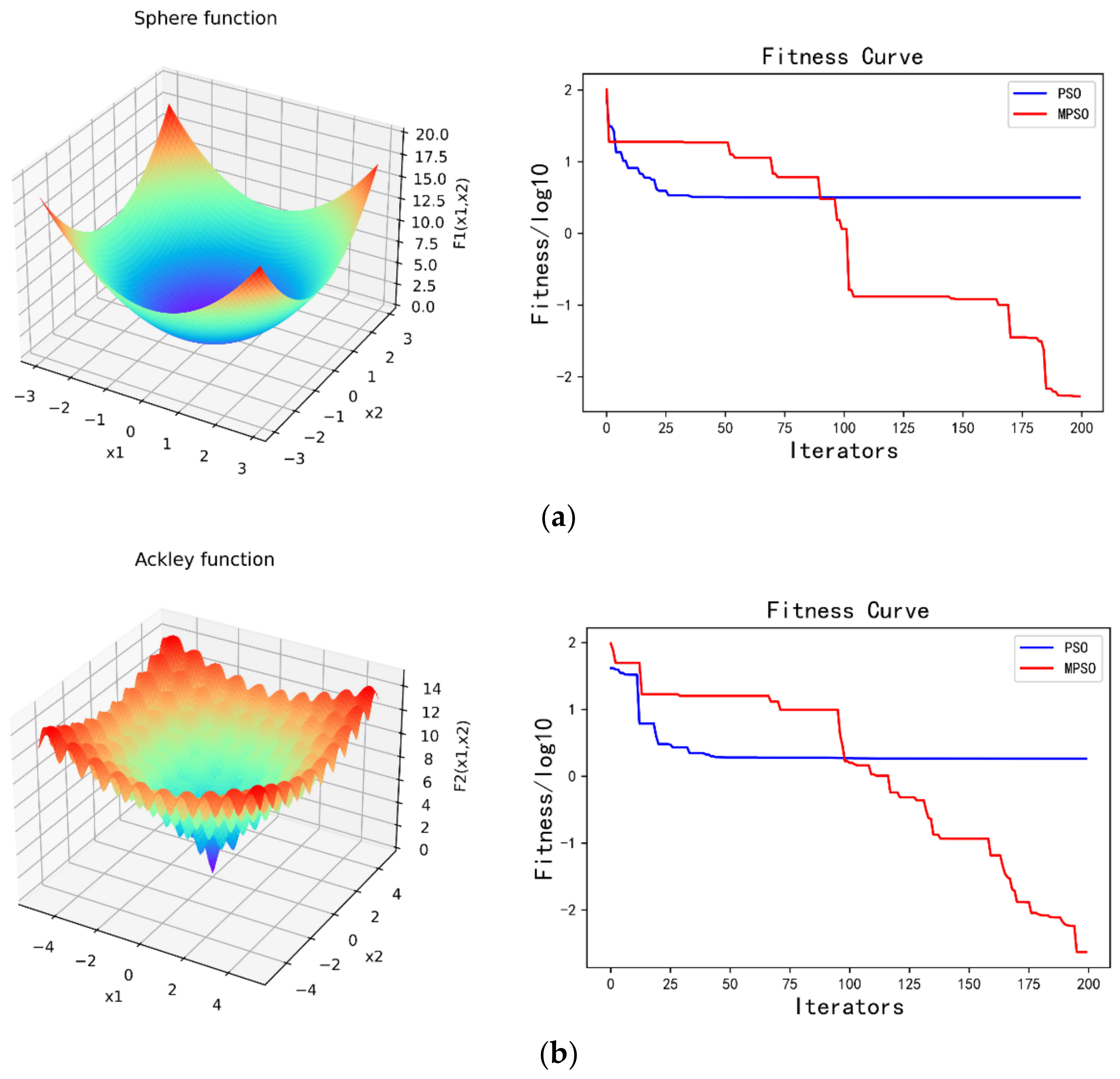
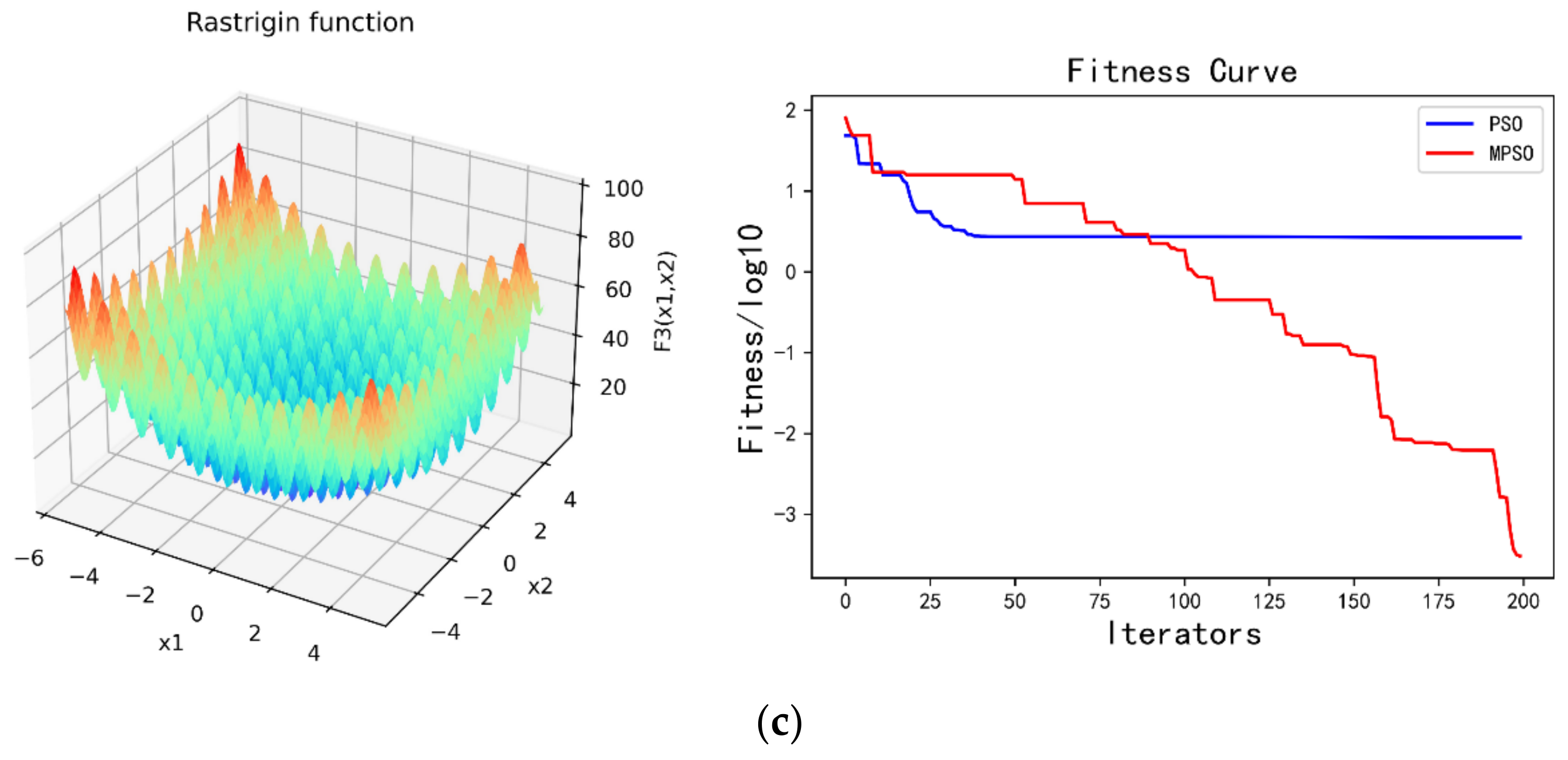
2.2. Modified Particle Swarm Optimization (MPSO)

In the earliest PSO algorithms, the inertia weights and learning factors are kept constant, which makes the models prone to premature convergence and falling into local optima. With the advancement and development of research, linearly adjusting the inertia weights and learning factors in PSO algorithms emerged. However, the linearly varying parameters still have the previous drawbacks. Therefore, we propose a modified particle swarm optimization (MPSO) with adaptive variation of nonlinearly adjusted parameters. The inertia weight ω and the individual particle learning factor c₁ in the algorithm decrease using a concave function, and the population learning factor c₂ increases using a concave function. The equation is as follows.

$$\begin{array}{c}\omega ={\omega }_{max}-\left({\omega }_{max}-{\omega }_{min}\right)\times \frac{4}{\pi }\arctan \frac{t}{t_{max}}\end{array}$$

(3)

$$\begin{array}{c} c_1=c_{1max}-\left(c_{1max}-c_{1min}\right)\times \frac{4}{\pi }\arctan \frac{t}{t_{max}}\end{array}$$

(4)

$$\begin{array}{c} c_2=c_{2min}+\left(c_{2max}-c_{2min}\right)\times \frac{4}{\pi }\arctan \frac{t}{t_{max}}\end{array}$$

(5)

where ${\omega }_{max},{\omega }_{min}$ are the maximum and minimum values of inertia weights, $c_{1max},c_{2min}$ are the maximum and minimum values of individual particle learning factors, $c_{2max},c_{2min}$ are the maximum and minimum values of population learning factors, and $t,t_{max}$ are the current and maximum of iterations.

Such an iterative strategy allows the algorithm to have a strong global search capability in the early stage and to enter the local search more quickly; it also allows a slow search in the later stage of the algorithm for a better local search. In the process of the nonlinear adjustment of the weights, we also refer to the “variation” operation in the genetic algorithm, where the probability of variation increases with the number of iterations, allowing the particles to enter other regions to continue the search and jump out of the local optimum. This can effectively expand the search range and reduce the probability of falling into the local optimum. The adaptive variation equation is as follows:

$$p_i=0.3+0.5\frac{t}{t_{max}}$$

(6)

where $p_i$ is the probability of the $ith$ particle variation. The PSO and MPSO algorithms were tested and evaluated using different benchmark functions; the parameters of the algorithms are shown in

Table 2. Parameter value of PSO and MPSO.

Algorithm	Parameter Setting
Common setting	Maximum iteration tmax = 200
	population size P = 5
PSO	$c_1=c_2=1.5$
	$\omega =0.9$
	$p=0.5$
MPSO	$c_{1max}=c_{2max}=2$
	$c_{1min}=c_{2min}=0.5$
	${\omega }_{max}=0.9$
	${\omega }_{min}=0.2$

. The parameters of the test functions are shown in

Table 3. Parameter of test functions.

Test Function	Name	Best
(1) Unimodal test functions
$F_1={{\displaystyle \sum }}_{i=1}^n{x}_i^2$	Sphere	0
(2) Multimodal test functions
$F_2=20+e-20\exp \left(-20\sqrt{\frac{1}{n}{{\displaystyle \sum }}_{i=1}^n{x}_i^2}\right)-\exp (\frac{1}{n}{{\displaystyle \sum }}_{i=1}^n\cos (2\pi x_i))$	Ackley	0
$F_3={{\displaystyle \sum }}_{i=1}^n\left[x_i^2-10\cos \left(2\pi x_i\right)+10\right]$	Rastrigin	0

.

Figure 1 presents the qualitative metrics for the F₁–F₃ functions, including 2D views of the functions and fitness curves. For the fitness curves in Figure 1, the blue line represents the PSO and the red line represents the MPSO. It can be seen that the convergence speed and accuracy of MPSO are better than that of PSO in test functions.

3. LSTM Network Based on Attention Mechanism

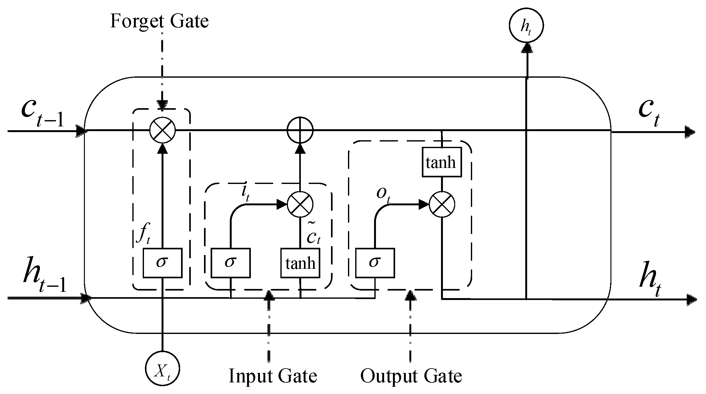
3.1. Standard LSTM Network

Input layer, hidden layer, and output layer are the components of a standard neural network. Standard neural networks, however, perform poorly in sequential tasks due to their inability to capture the trend aspects of sequence changes. RNNs are proposed as a solution for this issue. Traditional RNNs are limited, however, because they cannot handle the gradient expansion and gradient disappearance problems [27]. Long short-term memory (LSTM) and gated recurrent unit (GRU) proposed in [28] and [29], respectively, handle the aforementioned issues flawlessly. They are commonly employed in sequence issues. The standard LSTM structure is shown in the Figure 2.

The corresponding parameters are calculated as follows:

$$f_t=\delta \left(W_f\left[h_{t-1},x_t\right]+b_f\right)$$

(7)

$$i_t=\delta \left(W_i\left[h_{t-1},x_t\right]+b_i\right)$$

(8)

$$o_t=\delta \left(W_o\left[h_{t-1},x_t\right]+b_o\right)$$

(9)

$${\tilde{c}}_t=tanh\left(W_c\left[h_{t-1},x_t\right]+b_c\right)$$

(10)

$$c_t=f_t\times c_{t-1}+i_t\times {\tilde{c}}_t$$

(11)

$$h_t=o_t\times tanh\left(c_t\right)$$

(12)

$f_t,i_t$, and $o_t$ denote the forget gate, input gate, and output gate, respectively; W denotes the weight, the symbol $\left[h_{t-1},x_t\right]$ denotes the dimension of the input and the dimension of the hidden layer of the previous layer are summed in series, and b denotes the bias term; $\delta$ is the nonlinear activation function sigmod, and $W_f,W_i,W_o,b_f,b_i,b_o,$ and b_c are the parameters that the model needs to learn.

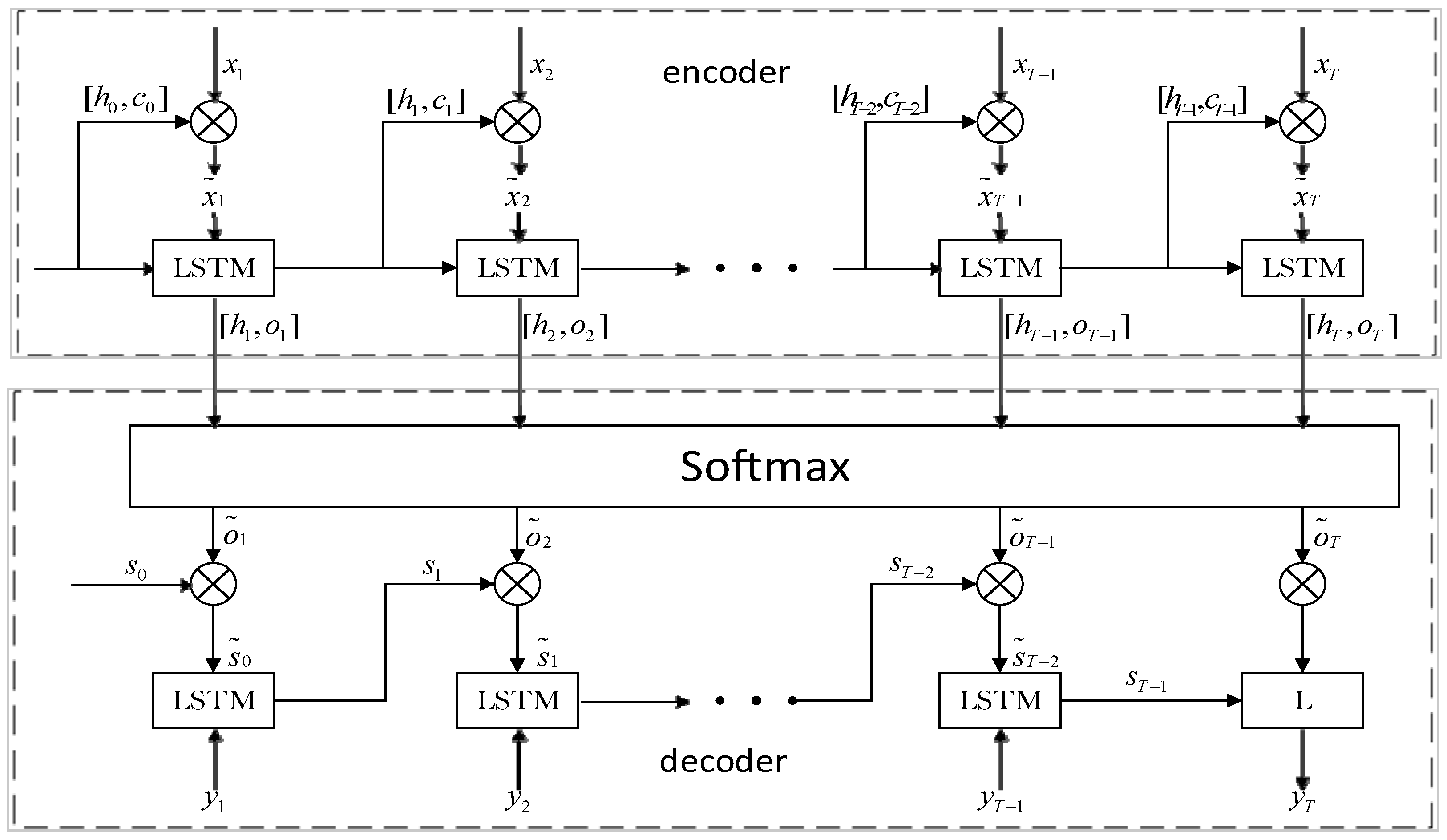
3.2. Attention Mechanism Model

The complete model framework is depicted in Figure 3. The model has two components: encoder and decoder. In the encoder step, we proposed to extract features using variable importance-aware input attention based on the LSTM structure. In the decoder step, an identical attention technique based on time windows is proposed by comparing the encoder’s output at each instant. Ultimately, the actual wind power is computed by combining all available data.

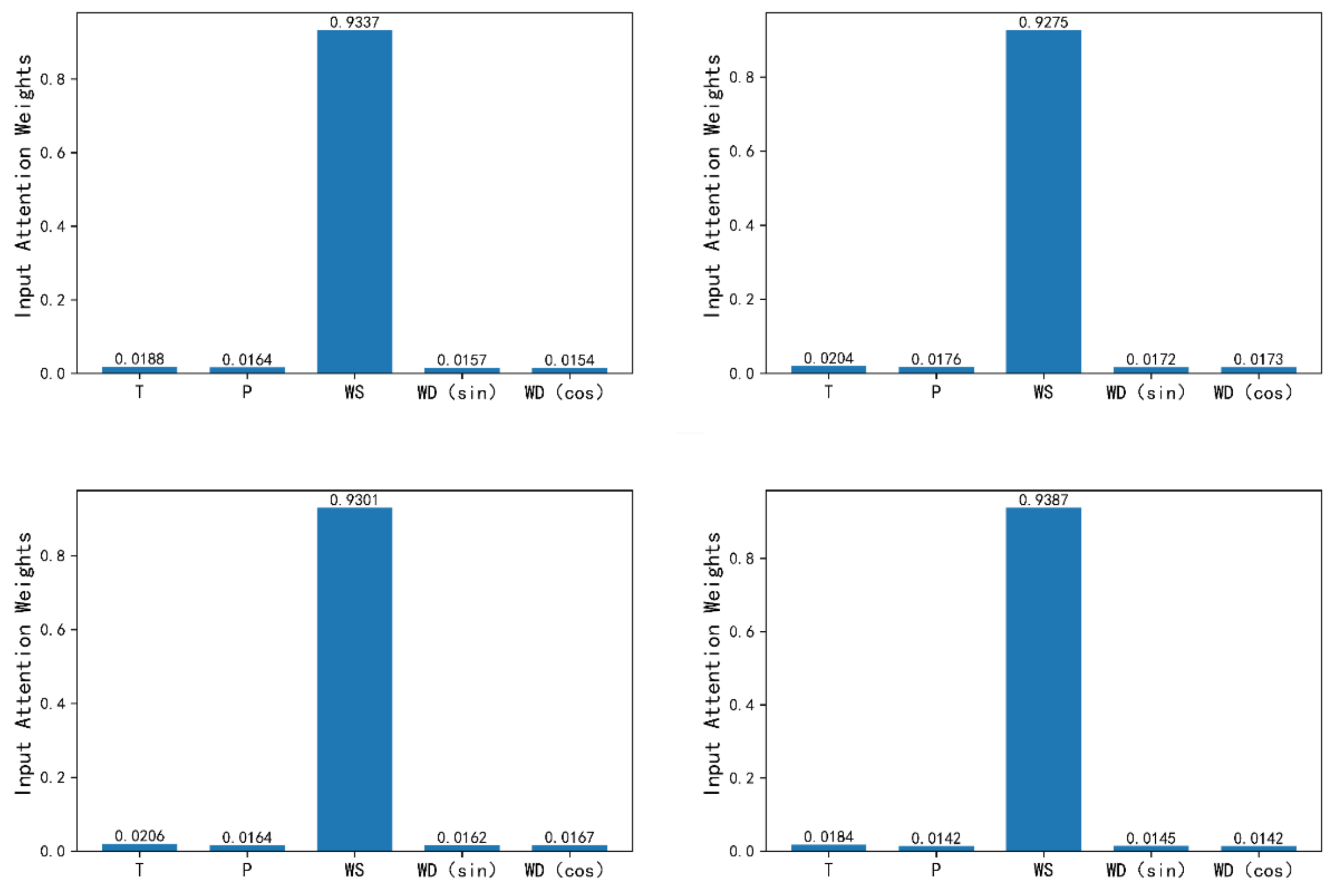
3.2.1. Input Attention Mechanism

The encoder step extracts datasets of feature from the input data. In this stage, the meteorological conditions are represented as a time series, denoted as $X=\left(x_1,x_2,x_3\dots x_t\dots x_T\right)$, where $x=\left(x_t^1,x_t^2,x_t^3\dots x_t^n\right)$ represents the n sub-features of the t step. For each time increment within the time window, using the following equation, useful features are extracted:

$$h_t=f_1\left(h_{t-1},c_{t-1},x_t\right)$$

(13)

where h_t is the current output state; $h_{t-1}$ and $c_{t-1}$ are the output state and cell state at the prior time t; x_t is the input at the current time; and f₁ is a nonlinear function representing the LSTM model.

The attentional feature parameter $e_t^i$ and the corresponding weight ${\alpha }_t^i$ for the $ith$ input at time t are determined by the following equation:

$$e_t^i=W_e\left[x_t,h_{t-1},c_{t-1},\right]+b_e$$

(14)

$${\alpha }_t^i=\frac{\exp \left(e_t^i\right)}{{{\displaystyle \sum }}_{i=1}^n\exp \left(e_t^i\right)}$$

(15)

The input to the LSTM model can then be calculated by the following equation:

$${\tilde{x}}_t=\left({\alpha }_t^1{x}_t^1,{\alpha }_t^2{x}_t^2\dots {\alpha }_t^n{x}_t^n\right)$$

(16)

Ultimately, the following equation is utilized to compute the input to the LSTM model based on the attention mechanism:

$$h_t=f_1\left(h_{t-1},c_{t-1},{\tilde{x}}_t\right)$$

(17)

f₁ denotes the LSTM network nonlinear function that dynamically adjusts the weather sub-feature weights at each moment through the attention mechanism.

3.2.2. Similar Day Attention Mechanism

The wind power generation and meteorological characteristics change constantly, but they have a certain trend of variation over a standard time series. To further capitalize on this variation pattern, we consider a new attention mechanism for similar days. This approach extracts the temporal trend characteristics by weighting the encoder output to determine the relationship between days with comparable characteristics, which is achieved by the following equation.

$$l_t=W_l\left[h_t,h_T\right]+b_l$$

(18)

$${\beta }_t=\frac{\exp \left(l_t\right)}{{{\displaystyle \sum }}_{t=1}^n\exp \left(l_t\right)}$$

(19)

where h_t is the output of the encoder at each time, and h_T is the output of the encoder at the last time T. W_l and b_l are the parameters obtained by the model through learning. l_T and β_t are the attention parameters and the corresponding weights obtained through the softmax layer. The final decoder input ${\tilde{o}}_t$ is determined by the following equation:

$${\tilde{o}}_t=\left({\beta }_1{h}_1,{\beta }_2{h}_2\dots {\beta }_T{h}_T\right)$$

(20)

The decoder also selects the LSTM network. First, the decoder step input ${\tilde{o}}_t$ and the hidden layer state $h_{t-1}^d$ and cell state $c_{t-1}^d$ obtained from Equation (13) are connected as the innovative LSTM structure hidden layer state ${\check{s}}_t$:

$${\tilde{s}}_t=W_o\left[{\tilde{o}}_t,h_{t-1}^d,c_{t-1}^d\right]+b_o t\in \left[0,T-1\right]$$

(21)

The input is $y_t=\left[y_1,y_2\dots y_{t-1}\right]$, and the features $h_{T-1}^d,c_{T-1}^d$ are fused by the LSTM network. The final wind power is determined using the following equation:

$$y_T=L\left(h_{T-1}^d,c_{T-1}^d,{\tilde{o}}_T\right)$$

(22)

where L is a three-layer neuronal layer with complete connectivity. The wind power prediction model is as follows:

3.3. Hyperparameters on the Network

Firstly, we test whether the hyperparameters in the LSTM network affect the results. The hyperparameters that need to be set in the LSTM network, such as the learning rate, the first and second hidden layer nodes, and the batch size experiments, are conducted with the parameters often used in the literature; other training parameters are consistent. The hyperparameters are shown in the

Table 4. Hyperparameter of different LSTM network.

Number of Model	Learning Rate	First Hidden Layer Nodes	Second Hidden Layer Nodes	Batch-Size
Hyperparameter-1	0.001	64	128	32
Hyperparameter-2	0.001	128	256	64
Hyperparameter-3	0.001	256	64	32
Hyperparameter-4	0.002	64	128	64
Hyperparameter-5	0.002	128	256	128
Hyperparameter-6	0.002	256	64	128

.

The training results of different networks for the same dataset are shown in the Figure 4.

It can be seen from the result chart that different hyperparameters have significant differences on the training results of the model. Therefore, the selection of hyperparameters is particularly critical to the quality of the model prediction results. It is not feasible to select hyperparameters by human experience.

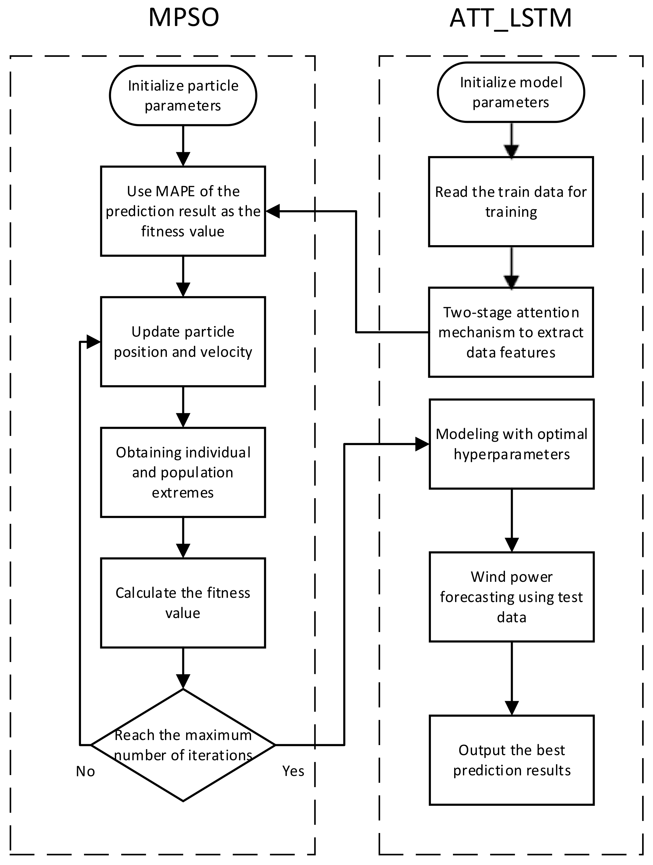
4. MPSO_ATT_LSTM Model

MPSO_ATT_LSTM modelling process:

Step 1:

Pre-process the experimental data and slice the processed data into training data and test data.

Step 2:

Initialize the relevant parameters of the modified particle swarm optimization (MPSO). Set up the maximum number of iterations $t_{max}$ of the modified particle swarm algorithm, the maximum and minimum values of inertia weights ${\omega }_{max}$ and ${\omega }_{min}$, the maximum and minimum values of individual particle learning rates $c_{1max}$ and $c_{1min}$, the maximum and minimum values of population learning rates $c_{2max}$ and $c_{2min}$, and the number of populations M. Set up the learning rate, the number of neurons in the first hidden layer and the second hidden layer, and the batch size in the LSTM model with the attention mechanism as the target optimization parameters of the improved particle swarm algorithm.

Step 3:

Form the corresponding particles and populations according to the parameters to be tuned, and construct the LSTM model with the attention mechanism with each particle corresponding to the initial parameters. Training is performed through the training data. As the fitness value of each particle, the mean absolute percent error (MAPE) of the results is used.

Step 4:

Real-time update individual particles and population optimal particle positions according to the MPSO algorithm.

Step 5:

Repeat the iterations until the maximum number of iterations is exceeded. Return the particle parameter corresponding to the best fitness and determine the value of the LSTM hyperparameter with the attention mechanism. Otherwise, return to step 4.

Step 6:

Substitute the obtained hyperparameters for the LSTM model with the attention mechanism. Wind power prediction has been performed on the test data.

The flow chart of the algorithm is as follows (see Figure 5).

The fitness curves are as follows (see Figure 6).

The MPSO_ATT_LSTM network hyperparameter search process is as follows (see Figure 7).

5. Experiment

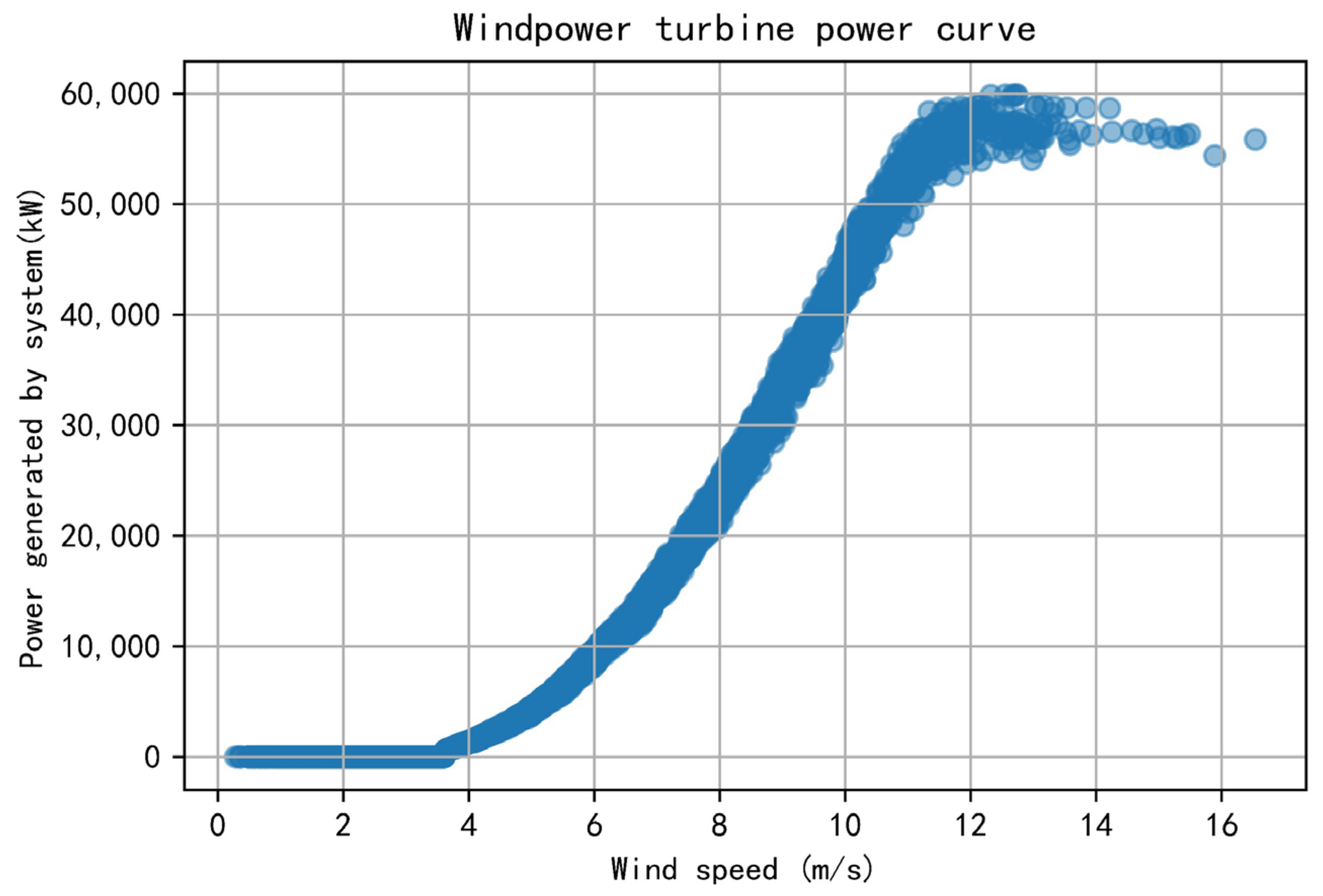
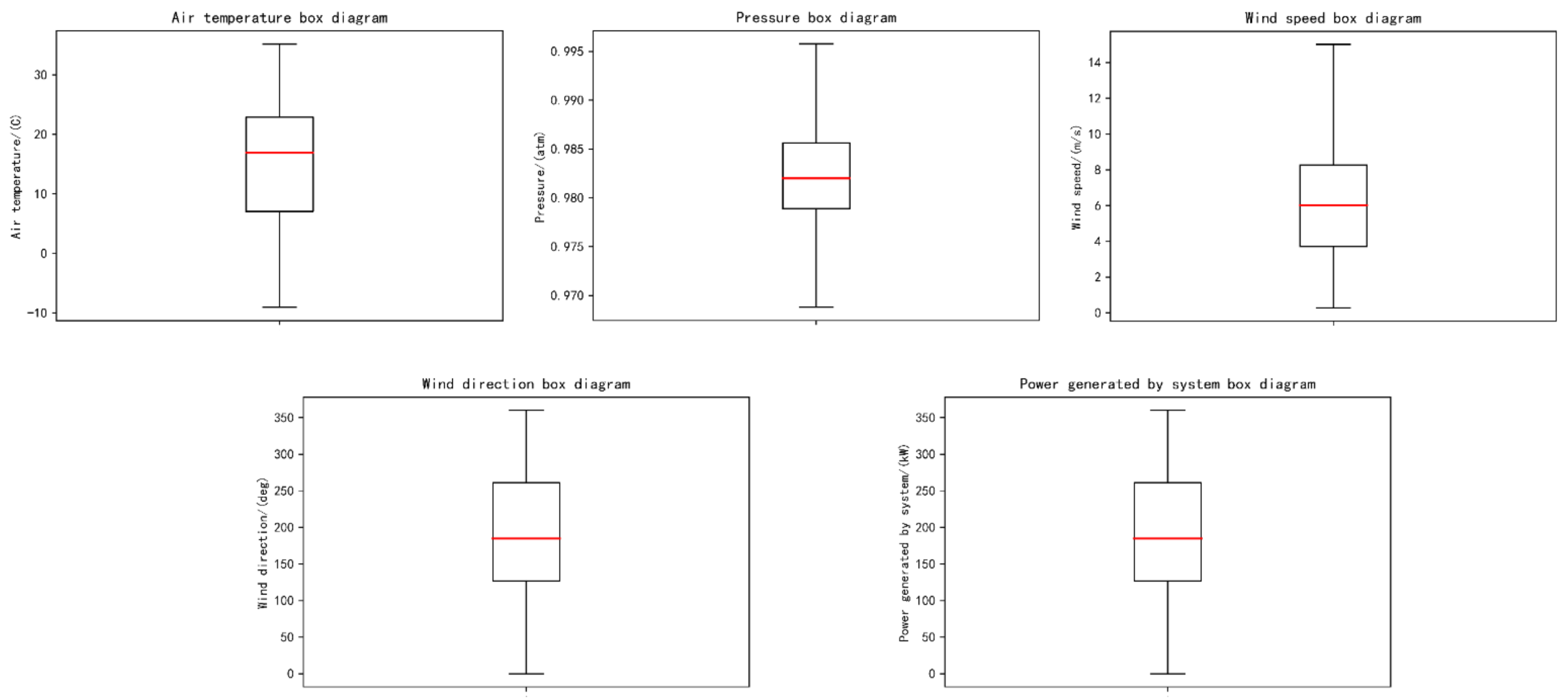
5.1. Dataset Description

National Renewable Energy Laboratory provided the wind power generating dataset used in this investigation [30]. This dataset contains hourly wind power, temperature, pressure, wind speed, and wind direction measurements from wind farms between 2007 and 2012. The initial five years of data were used as the training dataset. The data from the sixth year was used as the testing dataset (see Figure 8).

Before data processing, we analyzed the uncertainty of the data by using box diagrams; it can be seen from the result chart that the data is evenly distributed and stable (see Figure 9).

We have preprocessed the data before conducting the experiments:

(1)

Data cleaning: The original dataset contains some illogical or absent values. For instance, values of wind speed less than zero must be eliminated, and the missing values are filled with the mean of the upper and lower moments.

(2)

Data processing: Due to the fact that dataset has various units and orders of magnitude, the dataset is not comparable; they are standardized and normalized in advance. The wind direction takes values in the range of [0°, 360°]. Consequently, the wind direction data are converted to its sine and cosine values as the characteristics. Then, the transformed values are normalized to [−1, 1].

$${\mathrm{z}}_{\mathrm{t}}=\frac{x_t-\mathsf{\mu }}{\mathsf{\sigma }}$$

(23)

$$\tilde{x}=\frac{{\mathrm{Z}}_{\mathrm{t}}}{\max \left(\mathrm{z}\right)}$$

(24)

Normalization of wind power according to Equation (25):

$$\tilde{x}=\frac{x_t-\min \left(x\right)}{\max \left(x\right)}$$

(25)

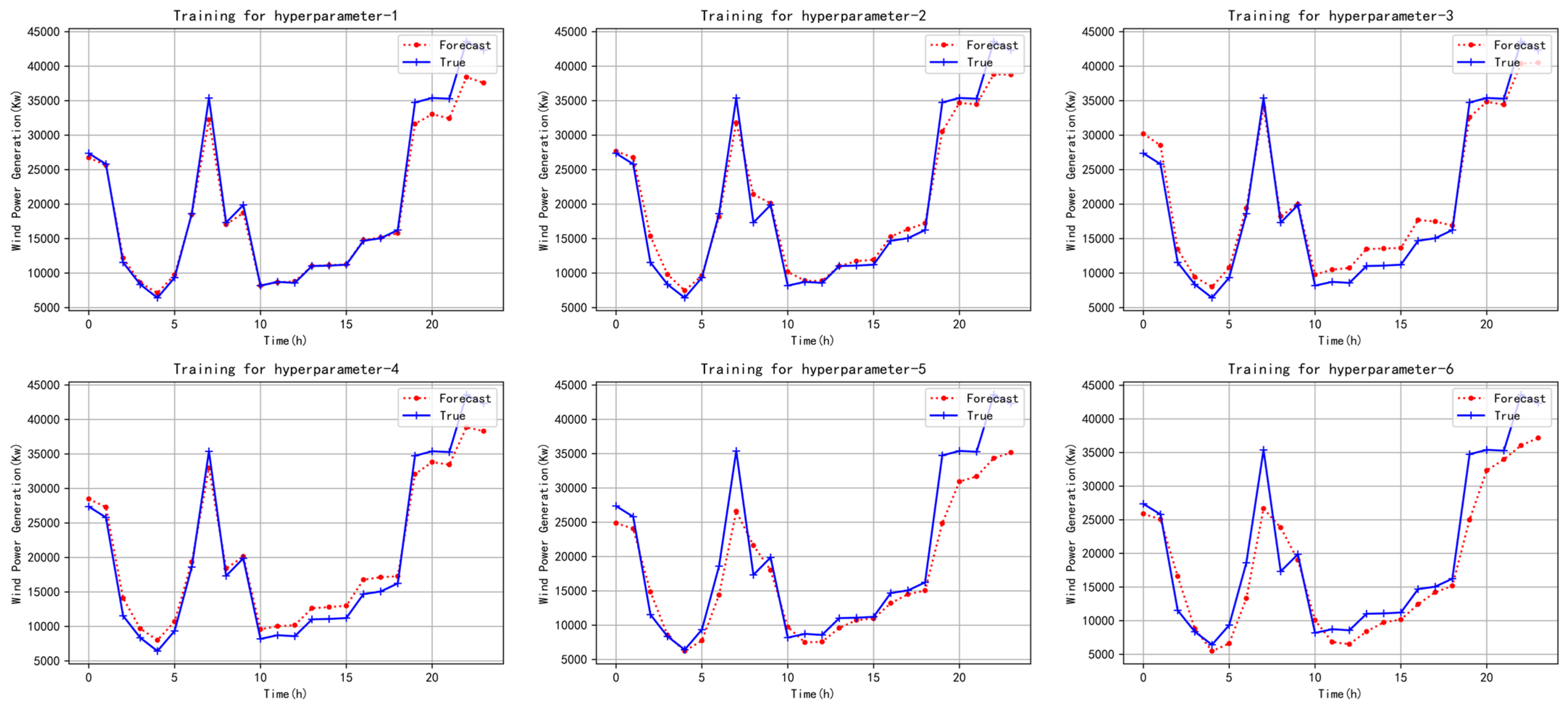
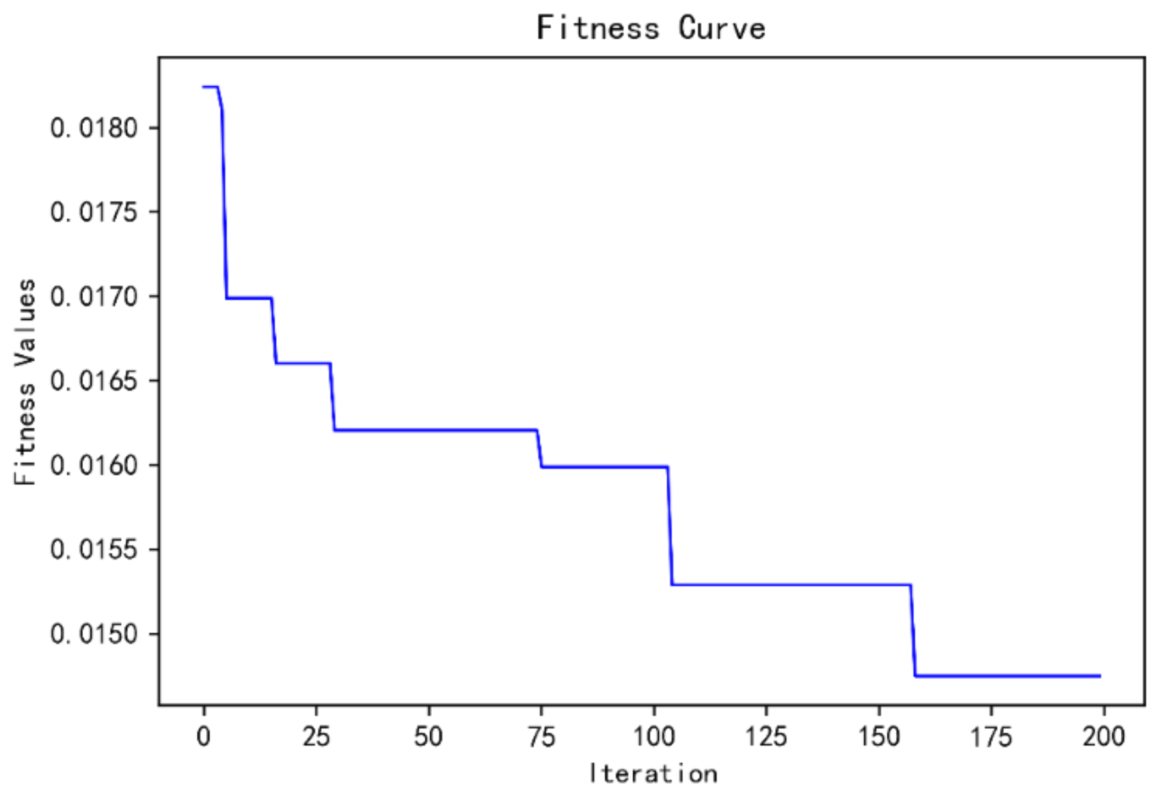
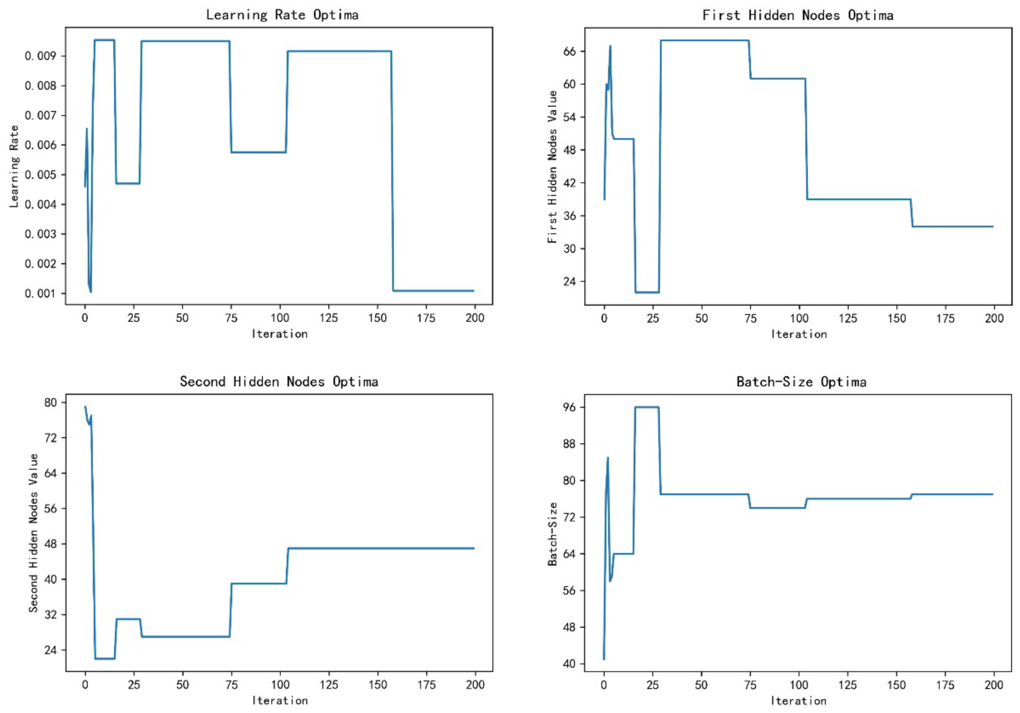
5.2. Training Process

The encoder and decoder have distinct functions; thus, they are optimized concurrently using two Adam optimizers with regularization. Adopting a learning rate that decreases exponentially throughout training allows for a rapid convergence of the model. The model with the greatest performance on the validation set is picked as the final model throughout the training process. This paper’s model implements Python as the programming language and Tensorflow as the deep learning framework. The parameters of the model are reported in

Table 5. Model parameters.

Parameters of the Model	Value
LSTM layers	2
Activation function	ReLU
Number of first hidden nodes	34
Number of second hidden nodes	48
Dropout	0.5
Learning rate	0.001
Learning decay rate	0.8
L2 regularisation	0.00001
Length of time windows	5
Batch size	78

.

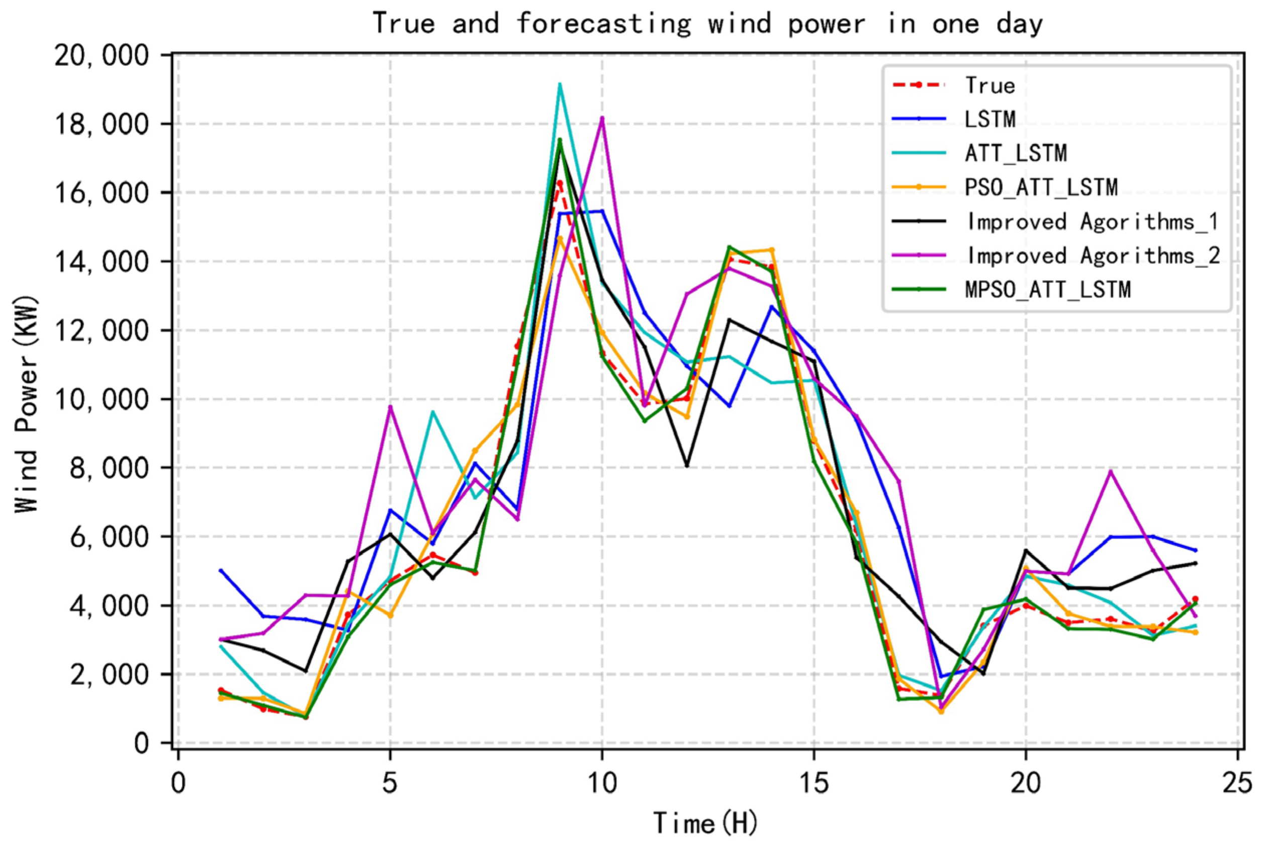
5.3. Wind Power Forecasting Assessment

Mean absolute percentage error (MAPE) and mean absolute error (MAE) are utilized to assess the accuracy of the suggested wind power prediction model by measuring the forecast results.

The mean absolute percentile error (MAPE) is used to measure forecast accuracy:

$$\mathrm{MAPE}=\frac{1}{\mathrm{N}}{\displaystyle \sum }_{\mathrm{I}=1}^{\mathrm{N}}\left|\frac{y_t-\widehat{y_t}}{y_t}\right|$$

(26)

The mean absolute error (MAE) reflects the actual situation of the errors:

$$\mathrm{MAE}=\frac{1}{\mathrm{N}}{\displaystyle \sum }_{\mathrm{I}=1}^{\mathrm{N}}\left|y_t-\widehat{y_t}\right|$$

(27)

$y_t,\widehat{y_t}$ are the true and predicted values of wind power at time t, respectively.

To value the proposed method, LSTM (network using the Adam algorithm), ATT_LSTM (LSTM model with the attention mechanism), PSO_ATT_LSTM (LSTM model fusing particle swarm optimization with the attention mechanism), MPSO_ATT_LSTM (LSTM model fusing modified particle swarm optimization with the attention mechanism), modified long short-term memory model [16] (Improved Agorithms_1), and improved artificial neural network [17] (Improved Agorithms_2) are used on the same dataset respectively for predictions. The prediction results are plotted as follows (see Figure 10).

Based on the evaluation index and prediction graphs, it can be determined that although all six approaches produced good results, the two-stage attention mechanism method based on MPSO-LSTM performs the best. It also reveals that both the modified particle swarm optimization algorithm and the two-stage attention mechanism improve the accuracy of model prediction greatly. In

Table 6. Model evaluation.

	MAPE, %	MAE, KW
LSTM	17.2	2423.6
ATT_LSTM	8.2	621.8
PSO_ATT_LSTM	5.9	359.3
Improved Agorithms_1	5.3	429.2
Improved Agorithms_2	6.5	373.6
MPSO_ATT_LSTM	4.6	211.5

, the error evaluation metrics of the approaches are provided. Obviously, compared with the existing and the latest literature methods, the model significantly improves the accuracy of prediction.

When the performance of the model on both the training and validation sets is satisfactory and it does not overfit, the model fit is deemed appropriate. Figure 11’s loss curve illustrates the degradation of the loss function over time. This curve may be used to predict if the model has been overfitted, underfitted, or is appropriately adapted to the training and testing datasets. Given the size of the training set, the loss function decays fast to a low value, as seen by the graph. Training and validation losses decline and level out approximately at the same time. Thus, the model accurately represents the wind power generation trends.

5.4. Two-Stage Attention Mechanism Explanation

Input attention mechanism: traditional machine learning techniques typically require variable correlation analysis to choose the most pertinent input features. By weighing each input variable, the input attention mechanism developed in this study automatically learns the relative importance of each variable throughout the training process and gives greater weight to the most important variables. This method resembles principal component analysis. According to the representation of input attention weights in the Figure 12, wind speed has the biggest impact on wind power generation, which is consistent with the findings of the current related study [31]. That study demonstrates the correctness of the input attention mechanism for selecting input variables.

Similar-day attention mechanism: The similar-day attention mechanism is utilized to acquire similar day weights by comparing the depth properties of the previous and current times inside the time window. The classic similar day technique compares expected data and previous data using the original statistical characteristics to obtain day-to-day information that is comparable. In this experiment, the similar day strategy provides comparable data through automatic model learning, hence reducing data preparation time. Although wind power fluctuates over time, it exhibits a definite trend. Therefore, the characteristics of the first few moments of the forecast point have different degrees of influence on the forecast results. In terms of influence weights, the closer the prediction time point is, the greater the influence on the prediction results. Similar daily attention weights do include this influence tendency, as demonstrated by Figure 13.

6. Conclusions

This paper proposes a two-stage attention-based LSTM model optimized by using a modified particle swarm optimization for forecasting wind power generation. By adding the attention mechanism, the importance of the input variables is automatically determined, hence eliminating the feature selection procedure required by conventional algorithms. On this basis, a similar-daily attention mechanism is proposed to extract the characteristics of the approaching time step in order to limit the impact of random fluctuations in wind power. Correlation outcomes that are computed by an end-to-end model can be applied to input variables directly. It avoids the clustering of data employed by the conventional method. Prediction accuracy is improved by introducing a modified particle swarm optimization to avoid the influence of artificially determined network hyperparameters. The simulation results on datasets show that the method in this paper has a higher prediction accuracy than the previous and most advanced algorithms. However, the hyperparameter search time is long, and we can consider improvements to the method to achieve parallel operation and reduce the network training time. At the same time, because most neural networks contain hyperparameters, this scheme is also applicable to other neural networks in principle and can be further verified in the future.

References

1. Gu, B.; Zhang, T.; Meng, H.; Zhang, J. Short-term forecasting and uncertainty analysis of wind power based on long short-term memory, cloud model and non-parametric kernel density estimation. Renew. Energy 2021, 164, 687–708. [Google Scholar] [CrossRef]
2. Xue, F.; Duan, H.; Xu, C.; Han, X.; Shangguan, Y.; Li, T.; Fen, Z. Research on the Power Capture and Wake Characteristics of a Wind Turbine Based on a Modified Actuator Line Model. Energies 2022, 15, 282. [Google Scholar] [CrossRef]
3. Ma, Y.-J.; Zhai, M.-Y. A Dual-Step Integrated Machine Learning Model for 24 h-Ahead Wind Energy Gneration Prediction Based on Actual Measurement Data and Environmental Factors. Appl. Sci. 2019, 9, 2125. [Google Scholar]
4. Donadio, L.; Fang, J.; Porté-Agel, F. Numerical Weather Prediction and Artificial Neural Network Coupling for Wind Energy Forecast. Energies 2021, 14, 338. [Google Scholar] [CrossRef]
5. Carvalho, D.; Rocha, A.; Gómez-Gesteira, M.; Santos, C. A sensitivity study of the WRF model in wind simulation for an area of high wind energy. Environ. Model. Softw. 2012, 33, 23–34. [Google Scholar] [CrossRef] [Green Version]
6. Kumar, A.S.; Cermak, T.; Misak, S. Short-term wind power plant predicting with artificial neural network. In Proceedings of the 16th International Scientific Conference on Electric Power Engineering (EPE), Koutynad Desnou, Czech Republic, 20–22 May 2015; pp. 548–588. [Google Scholar]
7. Kusiak, A.; Zheng, H.; Song, Z. Short-term prediction of wind farm power: A data mining approach. IEEE Trans. Energy Convers. 2009, 24, 125–136. [Google Scholar] [CrossRef]
8. Fan, G.; Wang, W.; Liu, C.; Dai, H. Wind power prediction based on artificial neural network. Proc. CSEE 2008, 28, 118–123. [Google Scholar]
9. Hu, Q. Impact of large-scale wind power access on grid dispatching operation. Sci. Technol. Wind. 2018, 14, 168. [Google Scholar]
10. Xu, Q.; He, D.; Zhang, N.; Kang, C.; Xia, Q.; Bai, J.; Huang, J. A short-term wind power forecasting approach with adjustment of numerical weather prediction input by data mining. IEEE Trans. Sustain. Energy 2015, 6, 1283–1291. [Google Scholar] [CrossRef]
11. Hu, Q.; Zhang, R.; Zhou, Y. Transfer learning for short-term wind speed prediction with deep neural networks. Renew. Energy 2016, 85, 83–95. [Google Scholar] [CrossRef]
12. Khodayar, M.; Wang, J.; Manthouri, M. Interval Deep Generative Neural Network for Wind Speed Forecasting. IEEE Trans. Smart Grid 2019, 10, 3974–3989. [Google Scholar] [CrossRef]
13. Bouktif, S.; Fiaz, A.; Ouni, A.; Serhani, M. Single and multi-sequence deep learning models for short and medium term electric load forecasting. Energies 2019, 12, 149. [Google Scholar] [CrossRef] [Green Version]
14. Song, H.; Dai, J.; Luo, L.; Sheng, G.; Jiang, X. Power transformer operating state prediction method based on an LSTM network. Energies 2018, 11, 914. [Google Scholar] [CrossRef] [Green Version]
15. Gundu, V.; Simon, S.P. PSO–LSTM for short term forecast of heterogeneous time series electricity price signals. J. Ambient. Intell. Hum. Comput. 2021, 12, 2375–2385. [Google Scholar] [CrossRef]
16. Son, N.; Yang, S.; Na, J. Hybrid Forecasting Model for Short-Term Wind Power Prediction Using Modified Long Short-Term Memory. Energies 2019, 12, 3901. [Google Scholar] [CrossRef] [Green Version]
17. Viet, D.T.; Phuong, V.V.; Duong, M.Q.; Tran, Q.T. Models for Short-Term Wind Power Forecasting Based on Improved Artificial Neural Network Using Particle Swarm Optimization and Genetic Algorithms. Energies 2020, 13, 2873. [Google Scholar] [CrossRef]
18. Bouktif, S.; Fiaz, A.; Ouni, A.; Serhani, M.A. Multi-Sequence LSTM-RNN Deep Learning and Metaheuristics for Electric Load Forecasting. Energies 2020, 13, 391. [Google Scholar] [CrossRef] [Green Version]
19. Zou, Y.; Feng, W.; Zhang, J.; Li, J. Forecasting of Short-Term Load Using the MFF-SAM- GCN Model. Energies 2022, 15, 3140. [Google Scholar] [CrossRef]
20. Zhu, A.; Zhao, Q.; Wang, X.; Zhou, L. Ultra-Short-Term Wind Power Combined Prediction Based on Complementary Ensemble Empirical Mode Decomposition, Whale Optimisation Algorithm, and Elman Network. Energies 2022, 15, 3055. [Google Scholar] [CrossRef]
21. Bahdanau, D.; Cho, K.; Bengio, Y. Neural machine translation by jointly learning to align and translate. arXiv 2014, arXiv:1409.0473. [Google Scholar]
22. Kennedy, J.; Eberhart, R. Particle swarm optimization. In Proceedings of the International Conference on Neural Networks, Perth, Australia, 27 November–1 December 1995; Volume 4, pp. 1942–1948. [Google Scholar]
23. Liu, X.; Yin, G. Risk Evaluation of Major Hazardous Sources Based on Improved PSO-LSTM School of Computer Science; Beihua Institute of Aerospace Technology: Langfang, China, 2021. [Google Scholar]
24. Viet, D.T.; Tuan, T.Q.; Van Phuong, V. Optimal placement and sizing of wind farm in Vietnamese power system based on particle swarm optimization. In Proceedings of the 2019 International Conference on System Science and Engineering (ICSSE), Dong Hoi City, Vietnam, 19–21 July 2019; pp. 190–195. [Google Scholar]
25. Kennedy, J.; Eberhart, R.C. A discrete binary version of the particle swarm algorithm. In Proceedings of the Computational Cybernetics and Simulation 1997 IEEE International Conference on Systems, Man, and Cybernetics, Orlando, FL, USA, 12–15 October 1997; Volume 5, pp. 4104–4108. [Google Scholar]
26. Khalil, T.M.; Gorpinich, A.V. Selective particle swarm optimization. Int. J. Multidiscip. Sci. Eng. 2012, 3, 2045–7057. [Google Scholar]
27. Bengio, Y.; Simrd, P.; Frasconi, P. Learning long-term dependencies withgradient descent is difficult. IEEE Trans. Neural Netw. 1994, 5, 157–166. [Google Scholar] [CrossRef] [PubMed]
28. Liu, Y.; Guan, L.; Hou, C.; Han, H.; Liu, Z.; Sun, Y.; Zheng, M. Wind Power Short-Term Prediction Based on, LSTM and Discrete Wavelet Transform. Appl. Sci. 2019, 9, 1108. [Google Scholar] [CrossRef] [Green Version]
29. Cho, K.; Merrienboer, B.; Gulcehre, C.; Bahdanau, D.; Bougares, F.; Schwenk, H.; Bengio, Y. Learning phrase representations using RNN encoder-decoder for statistical machine translation. arXiv 2014, arXiv:1406.1078,2014. [Google Scholar]
30. Draxl, C.; Clifton, A.; Hodge, B.-M.; McCaa, J. The wind integration national dataset (WIND) toolkit. Appl. Energy 2015, 151, 355–366. [Google Scholar] [CrossRef] [Green Version]
31. Li, B.; Peng, S.; Peng, J.; Huang, S.; Zheng, G. Wind power probability density forecasting based on deep learning quantile regression model. Electr. Power Autom. Equip. 2018, 38, 15–20. [Google Scholar]
Figure 1. (a) Sphere function; (b) Ackley function; (c) Rastrigin function.
Energies 15 04334 g001aEnergies 15 04334 g001b
Figure 2. Standard LSTM structure diagram.
Energies 15 04334 g002
Figure 3. Wind power prediction model.
Energies 15 04334 g003
Figure 4. Training for different hyperparameters.
Energies 15 04334 g004
Figure 5. The workflow of the proposed research work.
Energies 15 04334 g005
Figure 6. MPSO_ATT_LSTM fitness curve.
Energies 15 04334 g006
Figure 7. MPSO_ATT_LSTM network hyperparameter search process.
Energies 15 04334 g007
Figure 8. Historical data of the turbine power.
Energies 15 04334 g008
Figure 9. Data box diagram.
Energies 15 04334 g009
Figure 10. Wind power prediction results.
Energies 15 04334 g010
Figure 11. Loss value curve.
Energies 15 04334 g011
Figure 12. Input Attention Weights; T: Temperature; P: Pressure; WS: Wind Speed; WD(sin): Wind Direction sine; WD(cos): Wind Direction cosine.
Energies 15 04334 g012
Figure 13. Similar Day Attention Weights.
Energies 15 04334 g013