Abstract
Assessment of the wind turbine output power (WTG OP) during the operation and maintenance is one of the key indicators of operation quality evaluation. It is often carried out in the form of the wind speed-power curve. This form only considers the wind speed, and it is usually measured according to relevant IEC standards, e.g., IEC 61400-12, which has problems such as long measurement duration and harsh conditions. This study proposes a WTG OP assessment method based on SCADA data by using the regression-kriging algorithm. The influences of wind shear, turbulence intensity, and air density on the WTG OP were analyzed. Two regression-kriging output power models were built based on SCADA data (i.e., SCADA2power model) and wind resource parameters from met mast (i.e., wind2power model). According to the evaluation of the simulation result, it was found that the results of the two models are basically consistent. Based on the evaluation of historical data under normal operating conditions, the goodness of fitting output power of the two models is 99.9%. This shows that the regression-kriging-based wind turbine power performance assessment method based on SCADA data has an accurate prediction and the potential of general application in WTG OP evaluation.
1. Introduction
With the rapid development of renewable energy, especially the wind industry, and the advent of the Affordable Renewable Energy policy, the scientific operation of wind turbines has attracted more and more attention. Among them, the assessment of the output power of wind turbines is particularly important. The main requirements of output power mainly include the following points: (1) evaluation of wind turbine energy availability [1], (2) power generation and health monitoring [2], (3) wind power prediction [3], (4) frequency regulation of wind farms, etc. The current common practice for evaluation is based only on the wind speed-power curve [4], while considering only the wind speed. Many scholars have conducted in-depth research on this situation. Research [5,6,7,8] shows that the influence of environmental wind parameters such as turbulence intensity on the output power at some wind speed range can reach more than 10%. Obviously, these wind parameters at a specific site vary diurnally in different seasons and years. Hence, the WTG OP changes accordingly and causes large deviations in evaluating the energy availability of wind turbines. Moreover, the measured wind speed is disturbed by the near wake effect caused by the rotation of the wind turbine blades and cannot represent the free flow due to the position of the nacelle anemometer [9]. To address the above problems, two methods can be considered: (I) Measurement based on a met mast in the up-wind position of a specified turbine position in certain sites, referring to IEC61400-12-1 [10]. This method has the advantage of accurate evaluation results. However, it cannot be applied to every wind turbine in a wind farm and therefore, be widely applied in the output power evaluation for a whole wind farm due to high consumption of time and cost. (II) Correction, based on IEC61400-12-2 [9], the nacelle wind speed is corrected by the Nacelle Transfer Function (NTF). The power output of wind turbines is evaluated based on historical SCADA data. However, the conditions defined in this method are too demanding to apply directly, such as the installation position of nacelle anemometers, the nacelle size, and the terrain where wind turbines locate as well as the recommended linear NTF. In addition, it is hard to capture other factors which affect output power by nacelle wind measurement facility such as wind speed, turbulence intensity, wind shear, inflow angle, etc. Hence, how to accurately capture all factors is very challenging to massive application of the method [11]. Above all, how to accurately and cost-effectively capture factor variables of WTG OP and describe the WTG OPs through the captured factor variables becomes the challenging and the primary focus of this topic.
Regarding the above points, for a real-world large wind farm, application of the IEC 6100-12 method is difficult for wind turbine power performance assessment [12], especially election of the meteorological mast for all wind turbines are expensive [11]. However, the Power Curve Working Group makes use of the power deviation matrix (PDM) to quantitatively correct for power deviations in different meteorological conditions, such as air density, turbulence, shear, and so on [5]. It also shows that these factors cannot be ignored in the assessment of power characteristics. Given above considerations, there are two keys for WTG OP: (1) how to use or obtain unstable environmental conditions and variable operating conditions as input variables for WTG OP; (2) and the multidimensional variable power curve modeling method. For (1), past research demonstrates the benefit of using multivariate (WTG operation conditions source from SCADA and ambient conditions from met mast) in a power performance test [13,14,15,16,17]. Reference [13] used the blade pitch (SCADA), rotational speed (SCADA), temperature (met mast), and nacelle wind speed (SCADA) as the inputs for power curve assessment, and achieved more accurate results. Based on the variables introduced in Reference [13], Reference [14] added the statistical values of each input variable, such as average, standard deviation, maximum, minimum, and applied to wind turbines from the manufacturing plant with better results. Reference [15] only used the pitch angle and rotor speed from SCADA to describe the power curve. To sum, using more suitable SCADA variables and met mast variables to replace the single wind speed factor have become the trend of wind turbine power characteristic evaluation. For (2), the non-linear relationship between input variables and WTG OP needs modeling, commonly used non-parametric techniques [16], including the Gaussian process [18], neural networks [19], support vector machine [20], and polynomial LASSO regression [13]. They have demonstrated the effectiveness of machine learning in power curve modeling. This study proposes a WTG OP assessment method based on regression-kriging to address the problem of how to accurately and low-costly capture the affecting variables. Through considerable simulation data, it was verified that the variables accurately measured from the control system of wind turbines are equivalent to the wind resource parameters data obtained from the met mast in terms of output power. The regression-kriging power model was built based on historical data filtered from dataset in the production state and addresses the difficulty of obtaining the output power accurately. Finally, the above method was applied to the wind farm with power performance characteristic testing for verification.
2. Factors of Wind Turbine Power Output
The theoretical power of the wind turbine is defined as:
where P is the theoretical output power; ρ is the air density; v is the wind speed; A is the rotor swept area; and Cp is the power coefficient (related to the aerodynamic efficiency of the wind turbine blades, mechanical losses such as shafting, and electrical losses such as generators).
For a specific site, the inflow fluctuation in wind speed makes it necessary for general descriptions of wind conditions to include turbulence intensity [21], wind shear [22], and inflow angle. All of these have an impact on the actual output power of wind turbines. The inflow wind is not perpendicular to the rotor surface and the angle between inflow and the horizontal direction is the inflow angle due to the terrain factors. In the evaluation of the power characteristics of the wind turbine, the wind speed needs to be corrected according to the inflow angle:
where vi is the original wind speed; θ is the inflow angle; and ϕ is the tilt angle of the hub.
Considering the wind shear, the wind speed varies with the height from the surface; therefore, the wind energy acting on the wind turbine varies accordingly. The wind speed needs to be corrected as:
where veq is the rotor equivalent wind speed corrected with wind shear, n is the number of available measurement heights, vh is the wind speed at the reference height H, Zi is the middle height of the i-th segment, and the segment separation line is H − R < Zi < H + R. R is the radius of the rotor. A is the rotor swept area. Ai is the area at the target height Zi. The area can be calculated as:
The air density of wind farms changes accordingly due to the influence of diurnal and seasonal variation in temperature. For the pitch control turbine, the wind speed needs to be corrected according to the air density as:
where vi is the measured wind speed, ρi is the measured air density, and ρ0 is the reference air density.
For the effect of turbulence intensity on power output, the 10-min output power is corrected as:
where f(v) is the probability density function of the wind speed corrected by the inflow angle, wind shear, and air density, which is generally a Gaussian distribution. p(v) is a static power.
According to Equation (7), the output power of a certain type of wind turbine under different wind shear, air density, and turbulence intensity is simulated and calculated. As shown in the figures, turbulence intensity (Figure 1), wind shear (Figure 2), and air density (Figure 3) have a large impact on power output. When evaluating the output power of in-service wind turbines, the above-mentioned factors cannot be ignored. In addition, this implies that it is inaccurate to use only the wind speed of nacelle anemometer for the power output evaluation of wind turbines.
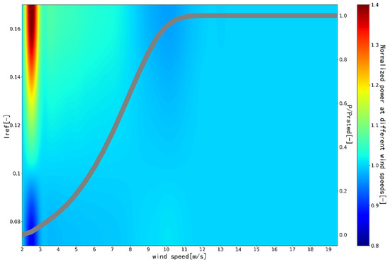
Figure 1.
The effect of turbulence intensity on WTG OP at different wind speeds (Iref is reference value of the turbulence intensity defined by IEC 61400-1:2019 [23], color axis = normalized power at different wind speeds).
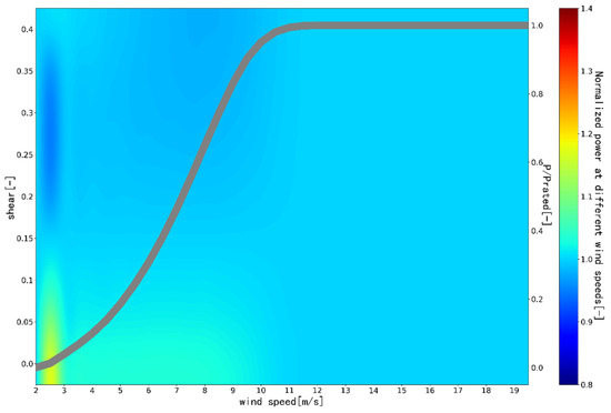
Figure 2.
The effect of wind shear on WTG OP (color axis = normalized power at different wind speeds).
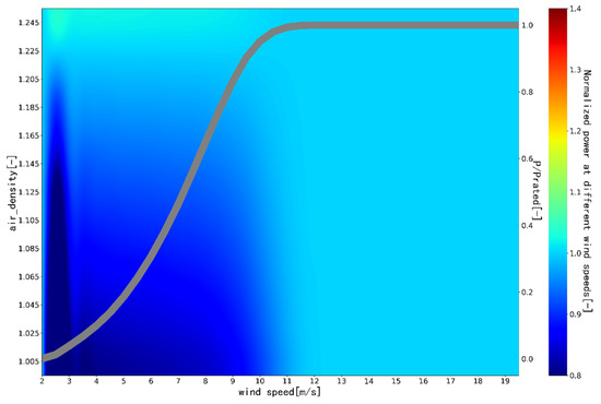
Figure 3.
The effect of air density on WTG OP (color axis = normalized power at different wind speeds).
3. Regression-Kriging Algorithm
Regression-kriging is a hybrid regression algorithm combining the Generalized Linear Model (GLM) and Kriging algorithm. It can well-characterize the random effects composed of systematic effects and regression residuals in n-dimensional space fields [24]. This characteristic is consistent with the characteristics of the WTG OP. The performance is that multi-dimensional environmental factors affect the output power, and the random fluctuation characteristics of the wind are integrated. Normally:
where f(X)Tβ is a generalized linear model composed of functional basis f = (fj, j = 1, 2, …, p) and its weights β = (βj, j = 1, 2, …, p). Z(X) is a Gaussian process function with a mean value of 0. Its covariance equation is defined as [25]:
where σ2 > 0 is the variance. R is the covariance equation, which depends on the distance of X − X′ and scale parameters θ.
On the assumption of the Gaussian process, the predicted value Y(x) corresponding to the observed actual value Y = (Y, i = 1, 2, …, m) and the unobserved input x is a joint normal distribution [26], namely:
where F = (fj(xi), i = 1, 2, …, m, j = 1, 2, …, p) is the regression matrix. R = [R(xi − xj, θ), i, j = 1, 2, …, m] is the correlation coefficient matrix between the training samples. r(x) = [R(x − xi, θ), i = 1, 2, …, m] is the cross-correlation coefficient matrix between the predicted value input and the training sample.
In summary, the regression-kriging model can be defined as:
where θ* and (σ2)* are the maximum likelihood estimates of scale parameter θ and variance σ2.
In this study, for the wind turbines output power model with multiple input variables, the quadratic basis (composed of the quadratic terms of the canonical basis) was used [18,24,27]. That is, for n-dimensional input variables X = x1, x2, …, xn, the functional basis is:
1, x1, x2, …, xn, xixj, ∀ i, j ϵ [1, n]
Its covariance function is an anisotropic exponential autocorrelation function [28].
where θi > 0, i = 1, 2, …, n is the scale parameter.
4. A Data-Driven Equivalence Validation of Input Variables
Regarding the power curve testing performed according to the IEC61400-12-1, it is highly challenging for power output measurement of wind turbines under all wind conditions due to constraints of site conditions and equipment type and accuracy. In contrast, the input variables of the data-driven output power model were validated by simulation data instead of wind resource parameters from met mast or SCADA system. The simulation data were extracted from a Monte Carlo sampling performed on a wide range of wind resource parameters combinations (i.e., wind speed, turbulence intensity, inflow angle, wind shear, air density, etc.) [28]. The simulated wind conditions were used as the input of a wind turbine design and simulation tool under the Normal Production Load Case (DLC1.2) of wind turbines to generate variables [29] such as: pitch angle, nacelle wind speed, rotor speed, nacelle acceleration-x, nacelle acceleration-y, active power. The result dataset is nominally identical to those collected from the SCADA data of a real wind farm under the corresponding wind conditions. The dynamics simulation time of a single case is 600 s and the amount of data in each wind speed bin fulfils the requirements in IEC6400-12-1. Scatter plots of each variable and the output power are shown in the Figure 4 and Figure 5.
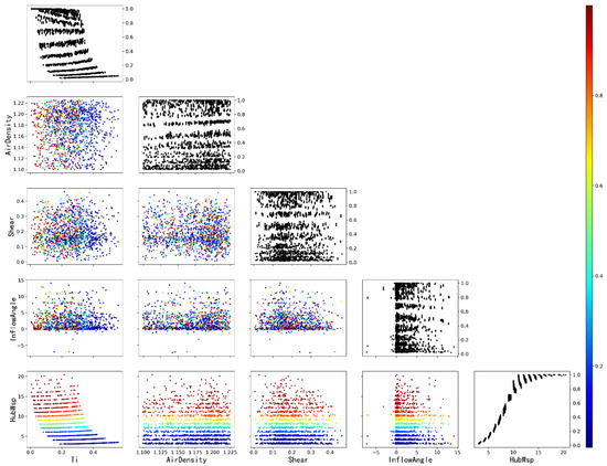
Figure 4.
Scatter plot of wind resource parameters from mast data vs. WTG OP, 2D matrix with so-called partial dependence plots of the WTG OP, this shows the influence of each varies from met mast (turbulence intensity, air density, wind shear, and inflow angle) on the WTG OP. The diagonal shows the effect of a single wind resource parameter on the WTG OP, while the plots below the diagonal show the effect on the WTG OP when varying two dimensions (color axis = normalized power at rated power).
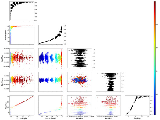
Figure 5.
Scatter plot of SCADA data vs. WTG OP, 2D matrix with so-called partial dependence plots of the WTG OP, this shows the influence of each varies from SCADA on the WTG OP. The diagonal shows the effect of a single SCADA parameter (blade pitch angle, rotor speed and nacelle accelerated velocity) on the WTG OP, while the plots below the diagonal show the effect on the WTG OP when varying two dimensions (color axis = normalized power at rated power).
A total of 70% of the dataset were used for building up the wind turbine power output model based on regression-kriging. The input of Model 1 is the ambient wind parameters of wind speed, turbulence intensity, inflow angle, wind shear, air density, and the output are the WTG OP (wind2power model). The input of Model 2 is the conventional SCADA data of wind turbines such as nacelle wind speed, rotational speed, pitch angle, nacelle acceleration, and the output are the WTG OP (SCADA2power model). Model testing is performed with the remaining data (i.e., 30% of the dataset) [30] and the results are shown in the Figure 6. For wind2power and SCADA2power models, the coefficient of determination compared the predicted output power of model with the simulated value are 0.98647 and 0.9984, respectively. Hence, the two models are equivalent in terms of output power prediction, which means the SCADA data can be used as an alternative of the met mast data to estimate the output power.
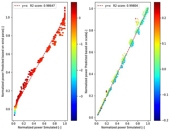
Figure 6.
The comparison result of the actual value and the predicted value of wind2power model and SCADA2power model.
5. Case Study
5.1. Test Case Overview
The wind farm of test case was installed with several wind turbines with rotor diameters (D) of 155 m and hub heights (H) of 110 m. In accordance with the relevant provisions of the IEC61400-12-1 standard, the met mast was installed to assess the output power performance characteristics of the wind turbine. The power measurement data were selected to validate various potential output power models. The wind turbines installed in this wind farm were the universal configurations from the same manufacturer. Its output power was normalized according to the rated power. The wind turbine T48 is used as the object of study. The position of the met mast and the wind turbine T48 is shown in the Figure 7. The met mast located in the dominant wind energy direction (NE) of the site, the distance from the wind turbine is 326 m, which is about 2.1 D. According to the relevant chapters of IEC 61400-12-1, the effective measurement sector is 85°~193°, as shown in Figure 8. The met mast was installed with various sensors such as wind speed, wind direction, temperature, humidity, pressure and so on at different heights and the configuration of these sensors is shown in the Figure 9.
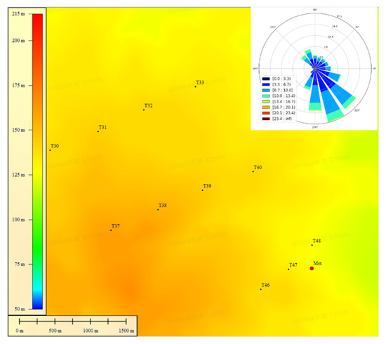
Figure 7.
The actual location map of the met mast and the wind turbines.
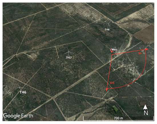
Figure 8.
Effective measurement sector of the met mast.
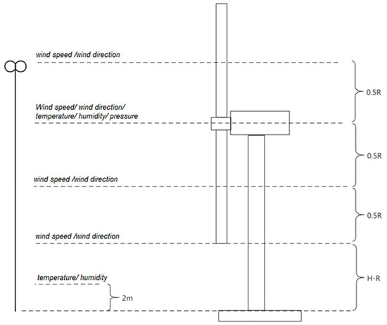
Figure 9.
Schematic diagram of installing sensors at different heights of met mast.
5.2. Data Processing
SCADA data and wind resource parameters data were cleaned, and the power curve and uncertainty were evaluated according to the data elimination rules in IEC61400-12-1. The evaluation results of the power curve before and after data cleaning are shown in the Figure 10 and Figure 11. The power curve was evaluated with the bin method. Uncertainty assessments also consider Type A and Type B.
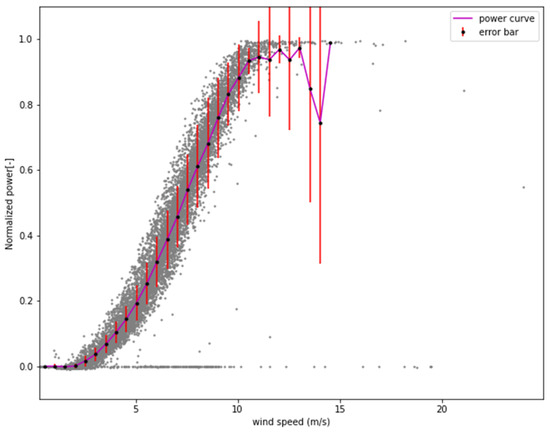
Figure 10.
Power curve based on database before cleaning.
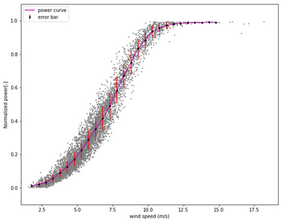
Figure 11.
Power curve based on database after cleaning.
In addition to cleaning the SCADA data and the wind resource parameters data, it is necessary to normalize the cleaned data. The following normalization methods are used in this study:
where max = 1, min = 0.
5.3. Regression-Kriging Model of WTG OP
To ensure that the wind measurement data is consistent with the wind resource parameters received by turbine T48, the test data in the valid sector was filtered and these data are synchronous data of wind turbines and met masts; totally, 1561 groups were selected (10 min sampling) and separated into training set and testing set with a ratio of 8:2. The coverage of the training set was checked synchronously. It can be seen from the Figure 12 that the data can cover the range from the cut-in wind speed to the rated wind speed of the wind turbine. It can be used for model training. Based on this, the following output power model was established as shown in the Table 1.
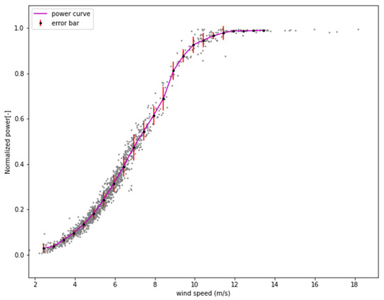
Figure 12.
Power curve based on training database.

Table 1.
Specific parameters of the established output power model.
5.4. Model Validation
In order to verify the effect of the above model in evaluating the WTG OP, the remaining 20% of the data that did not participate in the training was used for model verification. The SCADA2power model, wind2power model and nacelle power curve were used to predict the output power. The measured and predicted values are shown in Figure 13 and Figure 14. To evaluate the overall realization performance, some key indicators were selected, such as: mean absolute error (MAE), mean squared error (MSE), median absolute error (MAE), and explained variance score. The results are shown in Table 2. In general, the effect of WTG OP prediction is: SCADA2power model > wind2power model > nacelle power curve.
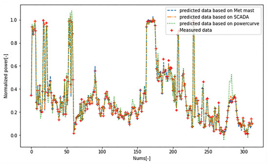
Figure 13.
Predictions from different models.
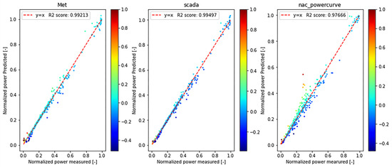
Figure 14.
Comparison of predicted and actual values of different models.
Table 2.
Evaluation results of different models.
The prediction results of three models were further analyzed. The frequency statistics of the residuals between the predicted values and the measured values of three models in the test samples are shown in Figure 15, and the residual statistics under different quantiles are shown in Figure 16. It can be concluded that the WTG OP mode using the regression-kriging algorithm is better than using the nacelle power curve to predict the output power. As shown in Table 3, according to the statistics of prediction values residuals of three models under different quantiles, it is further demonstrated that the WTG OP model with the regression-kriging algorithm is better than that predicted by the nacelle power curve.
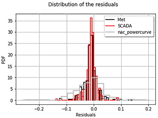
Figure 15.
Frequency statistics of residuals between predicted and measured values of the three models.
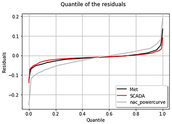
Figure 16.
Residual statistics at different quantiles for three model.
Table 3.
Statistical results of the residuals of the predicted values of the three models at different quantiles.
6. Conclusions
To assess the output power of wind turbines accurately cost-effectively, this paper studied a WTG OP assessment method based on SCADA data modeling with regression-kriging.
According to the analysis of external factors affecting the WTG OP, the major wind resource parameters are determined as wind shear, air density, and turbulence intensity. Hence, a sample of a wide range of wind resource parameters is established.
Through wind turbine dynamics simulations, the SCADA data under the normal power generation condition are generated. Comparing two types of wind2power models, it is concluded that the SCADA data consisting of operational status variables can be used as the input of the WTG OP evaluation model, and the effect is nominally identical to that of the wind resource parameters from met mast. This implies an implementation of WTG OP assessment avoiding met masts.
To establish the WTG OP models based on the regression-kriging algorithm, an operational wind turbine, T48, of a certain project was selected for field testing. Three models of the WTG OP were examined, including the SCADA2power, the wind2power model, and the nacelle power curve model. All three models were validated with measured data and results show that with either SCADA or multi-dimensional wind resource parameters as input, the accuracy of the WTG OP model based on regression-kriging is higher than that of using the nacelle wind speed-power curve. Moreover, when SCADA data and wind resource parameters data are used as input, the R2 between the predicted value and the measured value of both is greater than 99%. To a certain extent, it is completely universal. Therefore, for the modeling of the WTG OP, SCADA data can be selected as an alternative of the wind resource parameters data and contribute to reducing the met mast dependent modeling. Hence, the WTG OP assessment based on the SCADA2power model is a cost-saving method with limited equipment and shows the potential for remarkable economic value.
The current research only establishes the output power model under production cases, and it is necessary to further explore the models under different operating modes. Moreover, the wind farm in this case is non-complex terrain according to IEC standard. For complex terrain, the output power model based on regression-kriging needs further validation.
Author Contributions
Conceptualization, P.Z. and Z.X.; methodology, P.Z.; software, P.Z.; validation, P.Z., Z.X. and M.C.; formal analysis, P.Z.; investigation, P.Z.; resources, P.Z.; data curation, P.Z.; writing—original draft preparation, P.Z.; writing—review and editing, Z.X., S.G., M.C. and Q.Z.; visualization, S.G.; supervision, Z.X.; project administration, Z.X.; funding acquisition, Z.X. All authors have read and agreed to the published version of the manuscript.
Funding
This research was funded by Revitalization Talents Program of Liaoning Province, grant number XLYC2008005.
Institutional Review Board Statement
Not applicable.
Informed Consent Statement
Not applicable.
Data Availability Statement
The data that support the findings of this study are available from the corresponding author upon reasonable request.
Acknowledgments
The authors would like to thank the Liaoning Key Laboratory of Wind Power Generation Technology, together with the State Grid Liaoning Electric Power Co. Ltd.
Conflicts of Interest
The authors declare no conflict of interest.
References
- IEC. Wind Turbines—Part 26-2: Production-Based Availability for Wind Turbines; International Electrotechnical Commission: Geneva, Switzerland, 2014. [Google Scholar]
- Yan, J.; Zhang, H.; Liu, Y.Q.; Han, S.; Li, L. Uncertainty estimation for wind energy conversion by probabilistic wind turbine power curve modelling. Appl. Energy 2019, 239, 1356–1370. [Google Scholar] [CrossRef]
- Foley, A.M.; Hialeah, P.G.; Marvuglia, A.; Mckeogh, E.J. Current methods and advances in forecasting of wind power generation. Renew. Energy 2012, 37, 1–8. [Google Scholar] [CrossRef] [Green Version]
- Han, S.; Qiao, Y.; Yan, P.; Yan, J.; Liu, Y.; Li, L. Wind turbine power curve modeling based on interval extreme probability density for the integration of renewable energies and electric vehicles. Renew. Energy 2020, 157, 190–203. [Google Scholar] [CrossRef]
- Lee, J.C.Y.; Stuart, P.; Clifton, A.; Fields, M.J.; Housley, P. The Power Curve Working Group’s assessment of wind turbine power performance prediction methods. Wind. Energy Sci. 2020, 5, 199–223. [Google Scholar] [CrossRef] [Green Version]
- Hedevang, E. Wind turbine power curves incorporating turbulence intensity. Wind Energy 2014, 17, 173–195. [Google Scholar] [CrossRef]
- Wagner, R.; Courtney, M.; Gottschall, J.; Lindeloew-Marsden, P. Accounting for the speed shear in wind turbine power performance measurement. Wind Energy 2011, 14, 993–1004. [Google Scholar] [CrossRef] [Green Version]
- Lee, G.; Ding, Y.; Genton, M.G.; Xie, L. Power Curve Estimation with Multivariate Environmental Factors for Inland and Offshore Wind Farms. J. Am. Stat. Assoc. 2015, 110, 56–67. [Google Scholar] [CrossRef] [Green Version]
- IEC. Wind Turbines—Part 12-2: Power Performance of Electricity Producing Wind Turbines Based on Nacelle Anemometry; International Electrotechnical Commission: Geneva, Switzerland, 2013. [Google Scholar]
- IEC. Wind Turbines—Part 12-1: Power Performance Measurements of Electricity Producing Wind Turbines; International Electrotechnical Commission: Geneva, Switzerland, 2017. [Google Scholar]
- Wagner, R.; Pedersen, T.F.; Courtney, M.; Antoniou, I.; Davoust, S.; Rivera, R.L. Power curve measurement with a nacelle mounted lidar. Wind Energy 2013, 17, 1441–1453. [Google Scholar] [CrossRef] [Green Version]
- Ding, Y.; Kumar, N.; Prakash, A.; Kio, A.E.; Liu, X.; Liu, L.; Li, Q. A case study of space-time performance comparison of wind turbines on a wind farm. Renew. Energy 2021, 171, 735–746. [Google Scholar] [CrossRef]
- Astolfi, D.; Pandit, R. Multivariate Wind Turbine Power Curve Model Based on Data Clustering and Polynomial LASSO Regression. Appl. Sci. 2022, 12, 72. [Google Scholar] [CrossRef]
- Astolfi, D.; Castellani, F.; Lombardi, A.; Terzi, L. Multivariate SCADA Data Analysis Methods for Real-World Wind Turbine Power Curve Monitoring. Energies 2021, 14, 1105. [Google Scholar] [CrossRef]
- Janssens, O.; Noppe, N.; Devriendt, C.; van de Walle, R.; van Hoecke, S. Data-driven multivariate power curve modeling of offshore wind turbines. Eng. Appl. Artif. Intell. 2016, 55, 331–338. [Google Scholar] [CrossRef]
- Astolfi, D. Perspectives on SCADA Data Analysis Methods for Multivariate Wind Turbine Power Curve Modeling. Machines 2021, 9, 100. [Google Scholar] [CrossRef]
- Cascianelli, S.; Astolfi, D.; Castellani, F.; Cucchiara, R.; Fravolini, M.L. Wind Turbine Power Curve Monitoring Based on Environmental and Operational Data. IEEE Trans. Ind. Inform. 2022, 18, 5209–5218. [Google Scholar] [CrossRef]
- Guo, P.; Infield, D. Wind turbine power curve modeling and monitoring with Gaussian process and SPRT. IEEE Trans. Sustain. Energy 2018, 11, 107–115. [Google Scholar] [CrossRef] [Green Version]
- Karamichailidou, D.; Kaloutsa, V.; Alexandridis, A. Wind turbine power curve modeling using radial basis function neural networks and tabu search. Renew. Energy 2021, 163, 2137–2152. [Google Scholar] [CrossRef]
- Pandit, R.; Kolios, A. SCADA Data-Based Support Vector MachineWind Turbine Power Curve Uncertainty Estimation and Its Comparative Studies. Appl. Sci. 2020, 10, 8685. [Google Scholar] [CrossRef]
- Helbing, G.; Ritter, M. Improving Wind Turbine Power Curve Monitoring with Standardisation. Renew. Energy 2020, 145, 1040–1048. [Google Scholar] [CrossRef]
- Sumner, J.; Masson, C. Influence of Atmospheric Stability on Wind Turbine Power Performance Curves. J. Sol. Energy Eng. 2006, 128, 531–538. [Google Scholar] [CrossRef]
- IEC. Wind Energy Generation Systems—Part 1: Design Requirements; International Electrotechnical Commission: Geneva, Switzerland, 2019. [Google Scholar]
- Rasmussen, C.E.; Williams, C. Gaussian Processes for Machine Learning; MIT Press: Cambridge, MA, USA, 2005; ISBN 026218253X. [Google Scholar]
- Bjerager, P.; Krenk, S. Parametric sensitivity in first order reliability theory. J. Eng. Mech. 1989, 115, 1577–1582. [Google Scholar] [CrossRef]
- Dubourg, V. Adaptive Surrogate Models for Reliability Analysis and Reliability-Based Design Optimization. Ph.D. Thesis, Université Blaise Pascal—Clermont-Ferrand II, Clermont-Ferrand, France, 5 December 2011. [Google Scholar]
- Pandit, R.K.; Infield, D.; Kolios, A. Gaussian process power curve models incorporating wind turbine operational variables. Energy Rep. 2020, 6, 1658–1669. [Google Scholar] [CrossRef]
- Robert, C.P.; Casella, G. Monte Carlo Statistical Methods, 2nd ed.; Springer: New York, NY, USA, 2004; ISBN 9780387212395. [Google Scholar]
- Pelletier, F.; Masson, C.; Tahan, A. Wind turbine power curve modelling using artificial neural network. Renew. Energy 2016, 89, 207–214. [Google Scholar] [CrossRef]
- Santner, T.J.; Williams, B.J.; Notz, W.I. The Design and Analysis of Computer Experiments; Springer Series in Statistics; Springer: New York, NY, USA, 2003; ISBN 978-0-387-95420-2. [Google Scholar]
Publisher’s Note: MDPI stays neutral with regard to jurisdictional claims in published maps and institutional affiliations. |
© 2022 by the authors. Licensee MDPI, Basel, Switzerland. This article is an open access article distributed under the terms and conditions of the Creative Commons Attribution (CC BY) license (https://creativecommons.org/licenses/by/4.0/).