1. Introduction
Deployment of Advanced Reactor (AR) designs for energy generation is dependent upon cost effective Operation and Maintenance (O&M). Currently operating Nuclear Power Plants (NPPs) have much higher O&M costs due to higher manpower requirements for surveillance, involvement of various manual or complex procedures due to regulatory requirements, and lack of efficient O&M planning, while these concerns were aggravated by public opinion after the disaster at Fukushima Daichii, improvements on NPPs and their infrastructure are still a pressing concern. O&M activities such as startup, shutdown, or power level changes require the completion of comprehensive and time-intensive checklists and procedures for safety related equipment. Even more costly are O&M routine procedures and inspections that must be conducted based on a pre-planned procedure—independent of real need. Similarly, part replacement is also often dictated by a pre-planned program, instead of being based on field data followed by a risk-informed decision making process [
1,
2,
3]. These challenges become more pronounced with the associated aging processes in NPPs. O&M procedures could be dramatically improved by automating some of these processes using imaging and sensory information.
In all of these scenarios, the development of effective O&M strategies is dependent upon effective sensing of field variables (such as temperature, flow, strain, and neutron flux) and processing the data to assess safety and autonomous control; while developing an applicable model is feasible for normally operating systems, abnormalities introduced by external forces render these models unusable. Creating models for off-normal NPPs is much more difficult because of the inability to validate the predictive models of reactor systems and passive heat removal systems under seismic activity or similar external impact. The next generation of nuclear power plants, such as HTGRs (High Temperature Gas-cooled Reactors), have passive safety design features, but it is unclear whether their safety systems will perform as per design requirements in case of externally initiated events. Thus, a better approach needs to be prepared with better on-line monitoring systems and a sophisticated reactor safety management plan for advanced reactors.
The dynamic flow of heat between multiple reactor core components can be predicted by implementing a data learning tool on the kernels of the sensor and field locations within the core or material region of interest. Currently, there are two advanced HTGR designs with a graphite moderator and helium coolant planned for deployment—fuel moderator assemblies using prismatic blocks or fuel moderator assemblies using spherical pebbles. The main passive safety feature of these designs is that under off-normal conditions, they can passively dissipate heat to the external environment. This is based on the concept that the reactor vessel can be cooled by the external environment and internal decay heat within the reactor can be transferred to the vessel surface by heat conduction or radiation through the high thermal conductivity graphite fuel matrix. With the unpredictability of an abnormally functioning NPP in mind, there are many models that could be used to identify unknown temperatures to ensure the safety of the reactor core. There have been several attempts to adopt data learning models to solve inverse heat transfer problems [
4,
5]. Examples include the research of Yovanovich and Xu et al. [
6,
7]. Yovanovich covered the improvements on older data learning models and how geometry and thermal physics interact with regards to contact resistances, while Xu et al. proposed a new approach using the fractal dimensions of the conducting surface. The major issue shared by the models introduced by Yovanovich and Xu et al. is that both require the geometry of the conduction contact points to be known on a macroscopic and microscopic level. Without using data learning models, there are also more traditional approaches of identifying these unknown temperatures, such as finite element analysis (FEA) or a physics-based method. However, both 2D simulations and traditional physics based models also require a detailed investigation on the contact resistance values used for the data learning models. In addition, it is very difficult to produce accurate models using either method without extensive knowledge of the reactor’s current physical state. In order to overcome these limitations, a novel approach is introduced in this paper to quantify the effects of these line or point thermal contacts via a graphical model based on geometric connectivity instead of knowledge on the surface contacts. However, graphite fuel upon irradiation can undergo swell-shrinkage, thus changing block to block or pebble to pebble thermal contacts at a microscopic level. Modeling thermal resistance across these types of discontinuities involves complex empirical relations and grid-dependent numerical solutions near the boundaries, which are not reliable methods of solving such problems. To develop and demonstrate the effectiveness of multi-region assemblies filled with discontinuities, a problem setup is developed as described below.
This work mimics the HTGR cooldown scenarios but with the simplified geometry in the form of cylindrical rods, where the dominant form of heat transfer is conduction with ambient air providing convection cooling on the exterior of the holding vessel. The choice of materials such as alumina and quartz for this study was based on the lower thermal diffusivity of irradiated graphite and reducing spatial dimension to achieve comparable intra-rod time-constants as expected in HTGR fuel-moderator elements. This geometry allows the significant thermal response to occur predominantly in 2D geometry and demonstrates the performance of this machine learning method in 2D space before its future application towards more realistic reactor systems. Machine learning regression uses a large set of samples as data, where each data point consists of an input and output and the model identifies the relationship between the two. Two disjoint sets are needed for the machine learning model, the training set and the test set. The training set optimizes the model and trains it to yield desired results based off the change in input. The test set—which has data exclusive from the training set—is then entered into the newly trained model to assess the model’s performance. Although the entire space will be monitored using thermographic images, only a few randomly selected rods will be used for training the machine learning models. Using the remaining known temperatures for the rods as references, the model will then be able to accurately predict the temperatures of the unknown rods. The kernels used in this research have been devised to weight the relations between the rods using their thermal connectivity and the two sample observations’ closeness in time. More specifically, this investigation makes use of the Laplacian of a graph, a symmetric matrix that effectively captures various topological features of the underlying graph. A spatial regression algorithm is required to fuse the discrete signal response from some sensor locations and information on the rods’ physical properties to obtain the temperature map for the entire domain. Thus, if spheres are touching, they are then considered as point-contacts and if cylinders (such as the ones in our experiment) are touching each other along the curved surfaces, they can be considered as line contacts. Instead of modeling the heat transfer resistances across these point contacts or line contacts from physical models, these spatial or spatio-temporal regression models can be directly obtained from experimental data with high- or low-resolution instrumentation. The geometric connections and representative mathematical graphs in combination with the known data points are used in this work to construct a response function using a support vector regression algorithm. The response functions can then be used to predict responses for the unknown locations. In order to validate this algorithm, data which are not used in the support vector regression (SVR) are obtained during the experiments.
The presentation of this work involves the problem description with details on experimental setup, followed by procedure to generate experimental data for this study, the mathematical description of the predictive algorithm, and the discussion of results. The final section discusses the conclusions from this work.
2. Experimental Description
To develop and test a model for predicting temperatures in a simulated core during conduction cooldown, a high temperature experimental facility was constructed to record the temperatures of a randomly packed rod assembly over time [
8]. The following subsections outline the experimental setup and procedure.
Experimental Setup
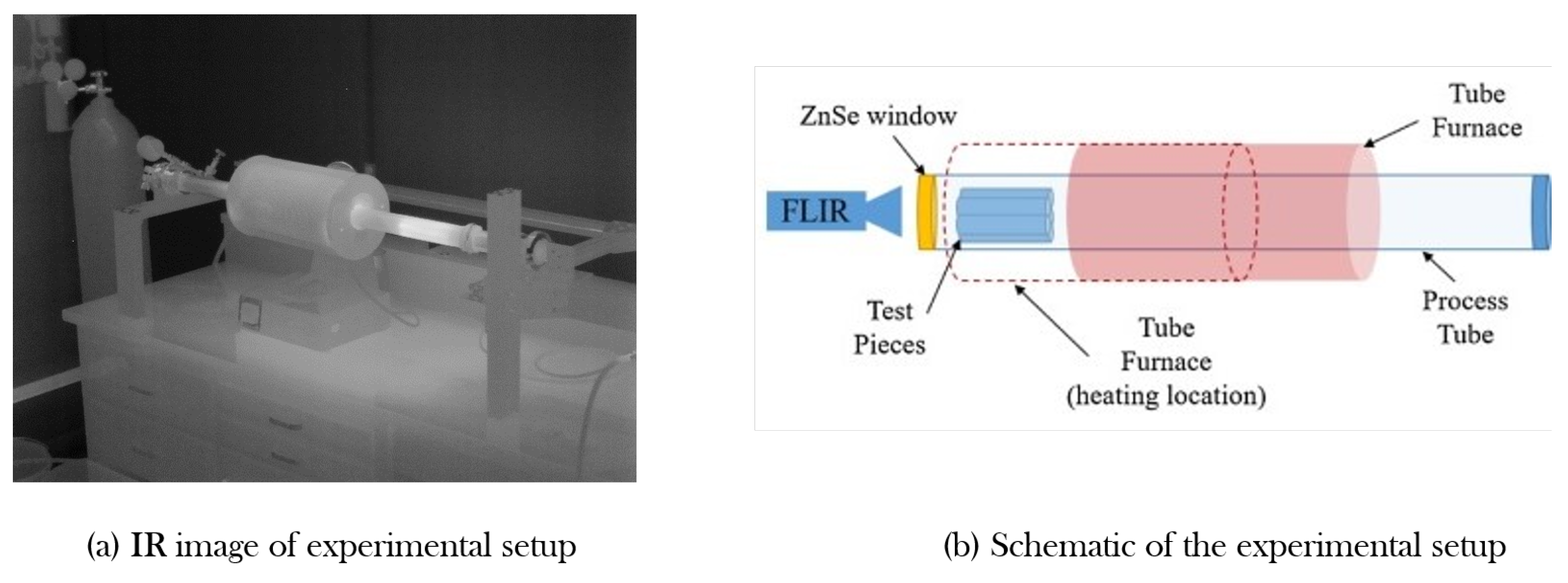
The experimental apparatus, built to analyze and test the regression model, consists of a quartz process tube and a radiative heater that is able to reach the desired temperature range (1000–1500 K). Depictions of this apparatus can be seen in
Figure 1. Quartz was chosen to hold the test samples within the furnace because of its infrared transmission and low thermal conductivity. The radiative heat from the electrical heater can transmit through quartz easily, ensuring that the sample quickly reaches the desired temperatures. Both ends of the tube were sealed using compression fittings which in turn allowed for KF style fittings to be attached. Although these connections would have been difficult to achieve without complex cooling equipment if a metal or ceramic tube had been selected, the low thermal conductivity of quartz resulted in end tube temperatures low enough that the compression fittings could achieve a seal by simply compressing their O-rings against the tube surface.
To allow for the long wave IR (LWIR) camera to measure the temperature variation inside the experimental domain, a custom ZnSe view port was commissioned to interact with the KF flange interface. As the ZnSe window has a substantial variation in the LWIR transmission as a function of wavelength, it was necessary to determine its transmission over the LWIR domain. By comparing two sets of images—one with the window, the other without—the correction factor for transmission can be obtained. For this process, a test piece was painted with a paint known to possess a constant emissivity in the LWIR spectrum over a range of temperatures [
9] for calibration purposes.
This setup provides a highly customizable apparatus for examining the effects of high temperature environments on test pieces of up to 4.6 cm in diameter. Utilizing a quartz process tube, samples of interest can be heated up to 1473 K in an inert environment ranging from a rough vacuum to pressures over 150 kPa. The complete experimental setup is shown in
Figure 1a.
Quartz and alumina were chosen for the two test assemblies to test the model’s versatility when used with different materials. The first assembly was used to test the machine learning model with a simpler geometry and only used seven rods of alumina. The second assembly uses 68 rods of graphite. Important thermal properties for quartz and alumina can been seen in
Table 1.
Both assemblies were placed in the quartz process tube near the IR camera’s minimum focal distance while being far enough away to avoid heat damage to the ZnSe window. After being carefully positioned inside the process tube, the process tube was vacuum sealed, and the radiative electrical heater turned on. Heating continued until all rods reached the desired steady state temperature of 1150 K for the 7-rod assembly or 1200 K for the 68-rod assembly. To initiate the assembly’s cooldown phase and record the actual data for experiments, the heater was unplugged and removed from the test section. This ensured that the residual heat from the heater did not reduce the heat removal from the test section.
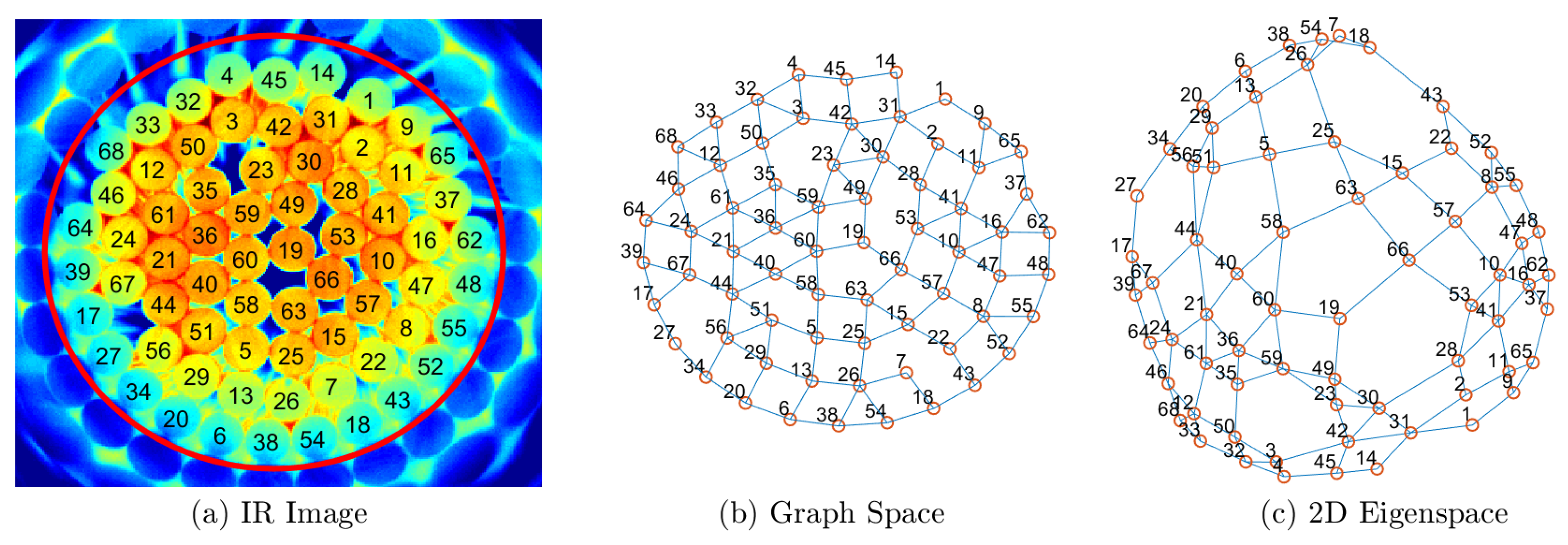
Figure 1b depicts the experimental setup, highlighting the sliding heater assembly. As the assembly cooled, temperatures were monitored and recorded for approximately 450 s using the IR camera. An example image observed of a single time snapshot of the test section during thermal transient is shown in
Figure 2a. Once the data were collected, the individual rods were identified and numbered, and the average temperature of each rod at each time step was recorded.
3. Machine Learning Model
Thermal analysis using a machine learning model requires the thermal conductivity of each rod in relation to one another to be established. By solidifying these relations in a numerical fashion, their edges can then be weighted to show their respective impacts on one another.
Machine learning models that are most frequently used in estimation tasks (i.e., neural networks, B-splines, or radial basis function networks) would use the physical coordinates of the rods, their temperatures , and other such properties as inputs. These approaches are infeasible for our proposed setup because the spatial coordinates of the rods do not capture the interconnectivity between the rods. A pair of rods may be physically close, but not in direct contact, meaning that their respective impact on one another is relatively minimal. Meanwhile, a pair of rods that are further apart could be tightly coupled thermally through multiple intermediate rods. Thermal images from the experiments are used to construct a graph network based upon adjacent connections between the rods. If the rod material and size varies then the graph network connections are expected to have non-uniform weighting. These weights can then be used to form a prediction for the unknown values in the assembly, but in this given study, all the rods were uniform in size and made of either quartz or alumina. The aspect ratio of the rods allowed this problem to be considered 2D, as the length of the rods was large enough to have boundary effects in the axial direction.
3.1. Graph-Based Learning
In order to effectively produce a method of weighting the interconnectivity between two rods, the proposed approach makes use of a scheme using algebraic graph theory described in the next section (
Section 3.1.1). This approach allows one to determine a kernel function
between any pairs of samples
and
. The kernel is an inner product operator defined in a feature space of the samples, and satisfies the usual properties of inner products. The feature space itself on which the inner products are defined is irrelevant to our discussion, although it is worthwhile to note that higher values of the inner product arise when the rods
i and
j are thermally tightly coupled and when time interval separating the samples
, is lower. These kernel products are used as inputs to the machine learning model which also uses the observed temperatures,
,
∈
, as training data. The specific machine learning model used is SVR, a model that relies on kernel functions as inputs instead of physical features to perform heat transfer analysis.
3.1.1. Graph Laplacian
The Laplacian,
, of a graph
G with vectors
V and edges
E,
, is the
symmetric matrix (
N being the cardinality of
V) defined as:
where
is the entry in row
i and column
j is defined as follows:
The Laplacian also takes into account the contact between the outer rods and the surroundings. In order to account for this connectivity with the surroundings, a node indexed 0 is added to symbolize the surroundings. The weighting factor between the rods connected to the surroundings is some number,
. Hence:
The Laplacian
is a singular matrix since
. Hence,
has an eigenvalue
. In case of a fully connected graph, all other eigenvalues are positive. The
N eigenvalues are sorted in ascending order, so that
. The spectral decomposition of
shows several interesting properties. For example, transforming the coordinates of the vertices in
V along the eigenvectors
and
produces a mapping where the
-norm distance between every pair of vertices reflects how closely connected the vertices are. In the present situation, these distances represent how thermally coupled the corresponding rods are, as shown in
Figure 2c.
3.1.2. Kernel Matrix
The exponential diffusion kernel [
10] of the Laplacian
is defined as:
where
is a spatial constant. The kernel
is positive definite and contains strictly non-negative entries. In other words:
Furthermore, it can be shown that given any two rods
:
Thus, the matrix
satisfies Mercer’s conditions [
11] and can be used for kernel-based regression methods as described below.
In order to extend the kernel inner product to samples that are also separated in time by an amount
, we include a factor
in the kernel, where
is a time constant. Under these circumstances, the kernel function between two samples can be stated as:
The graph
is constructed in the following manner. Each vertex in the set
V corresponds to a rod. Since the data used for the second test section involved a total of 68 rods (see
Figure 2), the cardinality of
V was also
. For every pair of rods
i and
j that were in direct contact, the representing edge
belongs to
E. Since the radii of the rods were equal, the edge weights between touching rods were kept at unity.
3.2. Support Vector Regression
Given the points
, with
denoting the temperature of rod
i, the objective is to obtain an approximator
. SVR, which is known to perform optimal estimation while minimizing the VC-dimensionality, was used [
12].
3.2.1. Primal Form
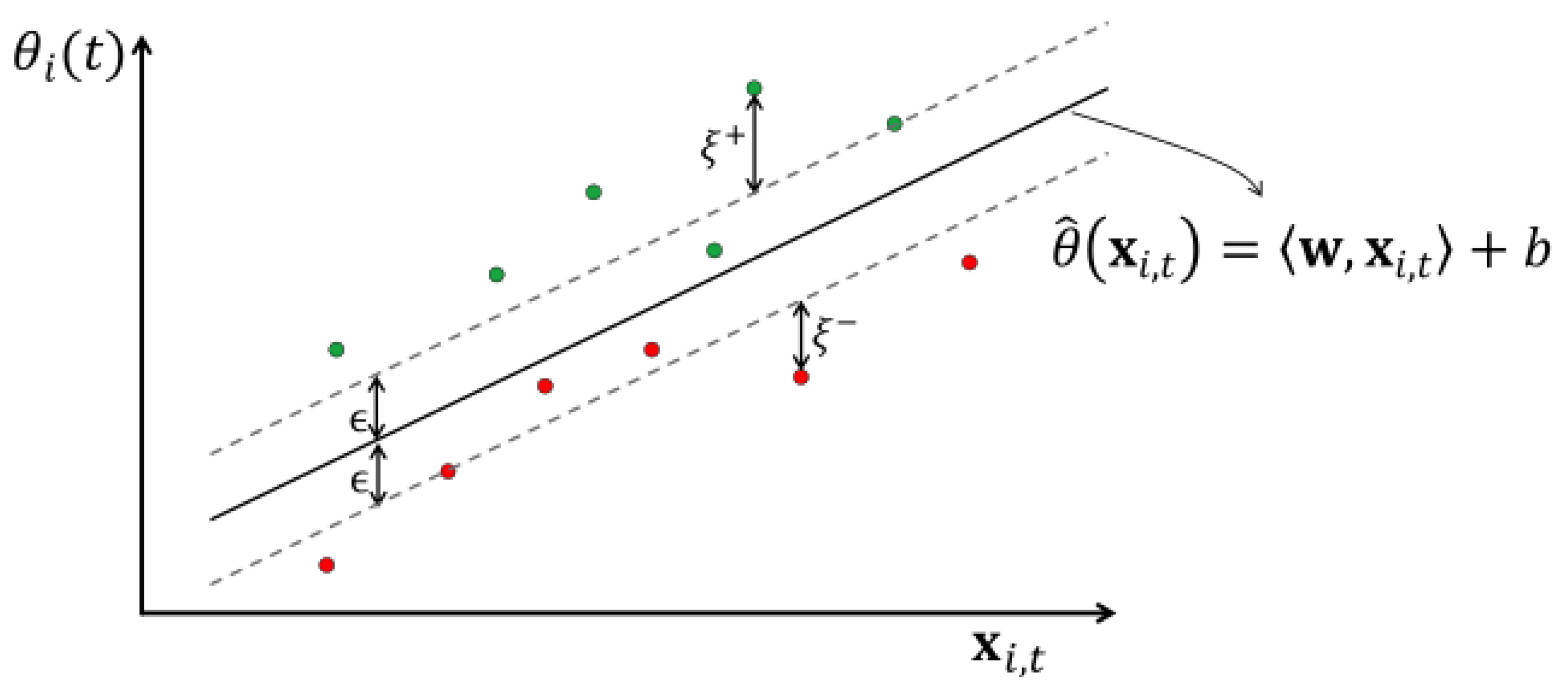
Two sets of slack variables can be used, for points above the regression surface, and for points below it. Furthermore, we apply a threshold . With the -insensitive loss function being the objective, the problem is formulated as below.
Subject to:
where
is a vector of weights and
b is the hyperplane bias vector.
3.2.2. Dual Form
Introducing Lagrange multipliers and for the constraints in the primal formulation above, the dual can be readily obtained as below.
Let
be a vector consisting of both sets of Lagrange multipliers as shown below:
Using
, the kernel matrix
can be rewritten for the above dual problem as:
Let
be the dual variable sets corresponding to rods whose temperatures are in the active region. It can be shown that the bias
b of the primal form can be obtained as:
The weight vector
of the primal form can be shown to be as follows:
3.2.3. Training and Testing Datasets
In order to predict rod temperatures, both spatial and temporal inputs are required. In this application, both training dataset
and
use
, where
i is the rod index and
t denotes the time instance. For example, the training dataset for the 68 rod setup consists of the temperatures for 34 randomly selected rods (
) at each time instant across the entire time domain, as well as the remaining 34 rods where the temperature will be unknown (
) from the initial time to some time,
. As addressed earlier, the temperature
of the surroundings is treated as an extra training sample, with index
. Together these samples make up the training set:
Furthermore, testing data can be mathematically written as:
3.2.4. Unknown Temperature Estimation
Using the dual formulation, it can be seen that need not be determined explicitly. This is because during regression of unknown points , only kernels are required, and the weight vector itself is a linear combination of the of the rods with known temperatures.
Given any rod
j with unknown temperature
, the estimated temperature
is determined as follows:
The SVR algorithm then uses the extended kernel matrix
. For any sample datapoint
, with corresponding temperature
, the purpose of the SVR formulation is to obtain temperature estimate
. The estimate
and
, which are denoted as
and
, can be formulated as:
If
, no penalty is incurred. The SVR formulation leads to the
as:
Figure 3 shows the formulation of a hyperplane,
from known rod temperatures using the loss functions,
and
, and slack variables,
and
.
4. Results and Discussion
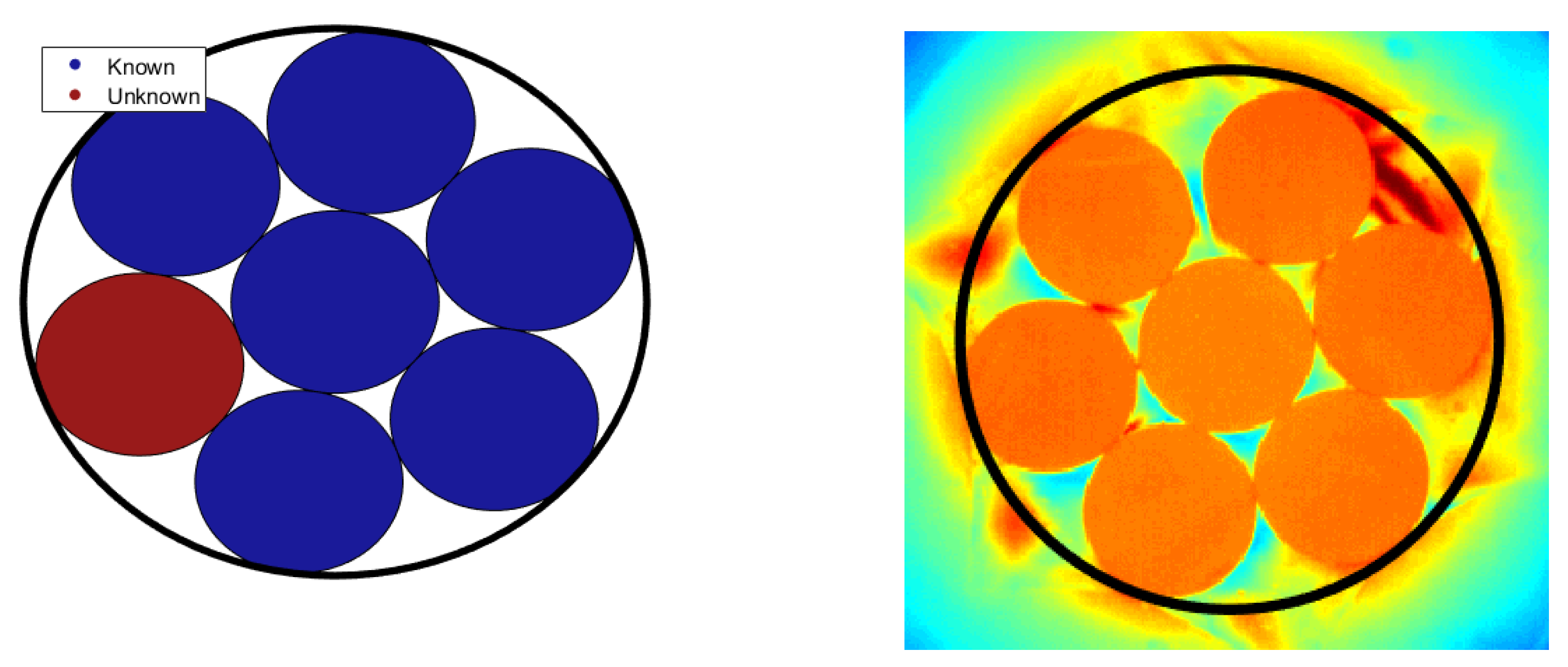
To test the efficacy of the support vector regression, a simple geometry of seven alumina rods was used. The training dataset consisted of the temperatures for all seven rods over the first 300 s of cooling and the temperatures of six over the entire cooling time. This training set was used to train the kernels in order to predict the temperature of the remaining rod over the final 1200 s of the cooling period. The rods used for training, as well as the test rod, are shown in
Figure 4.
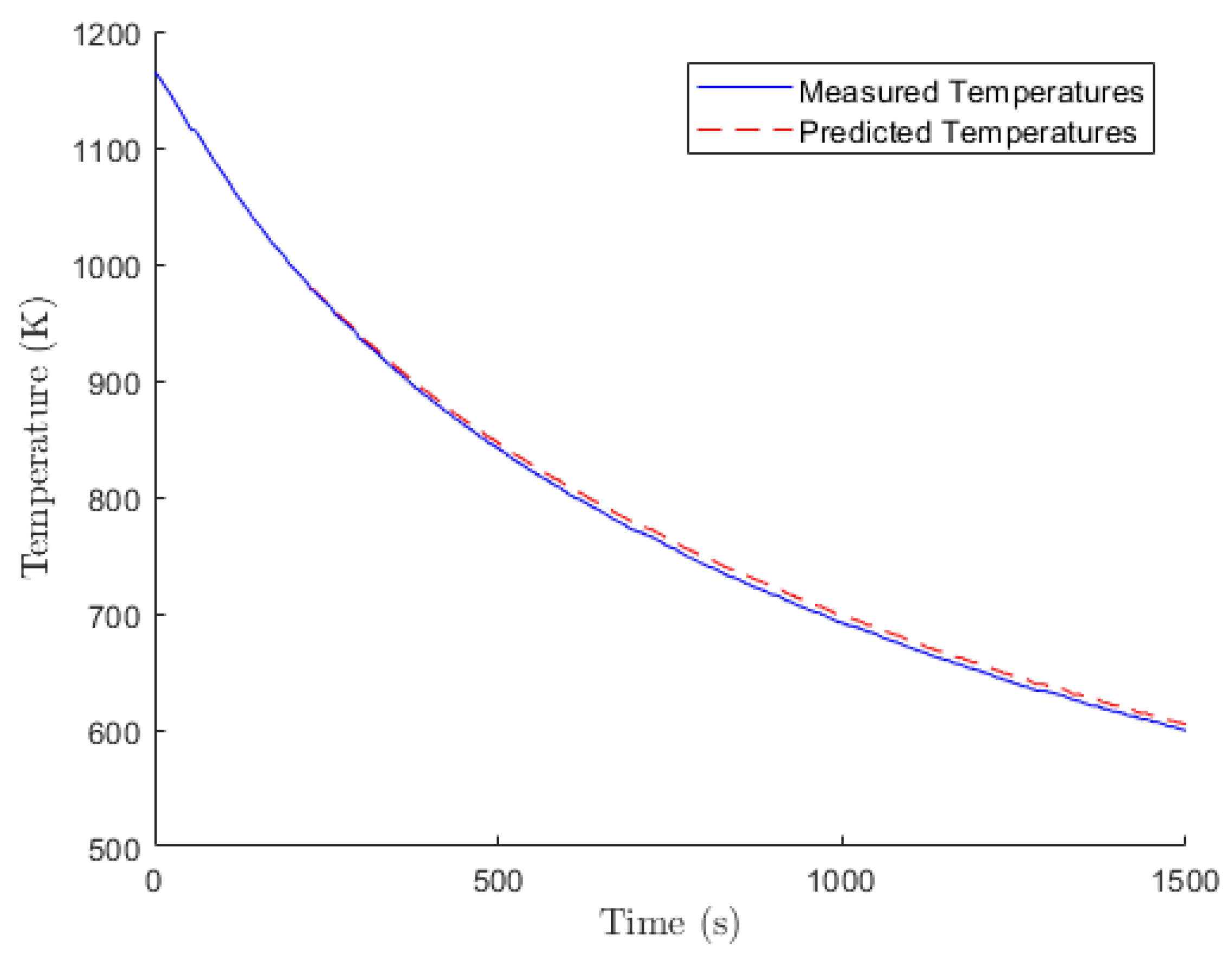
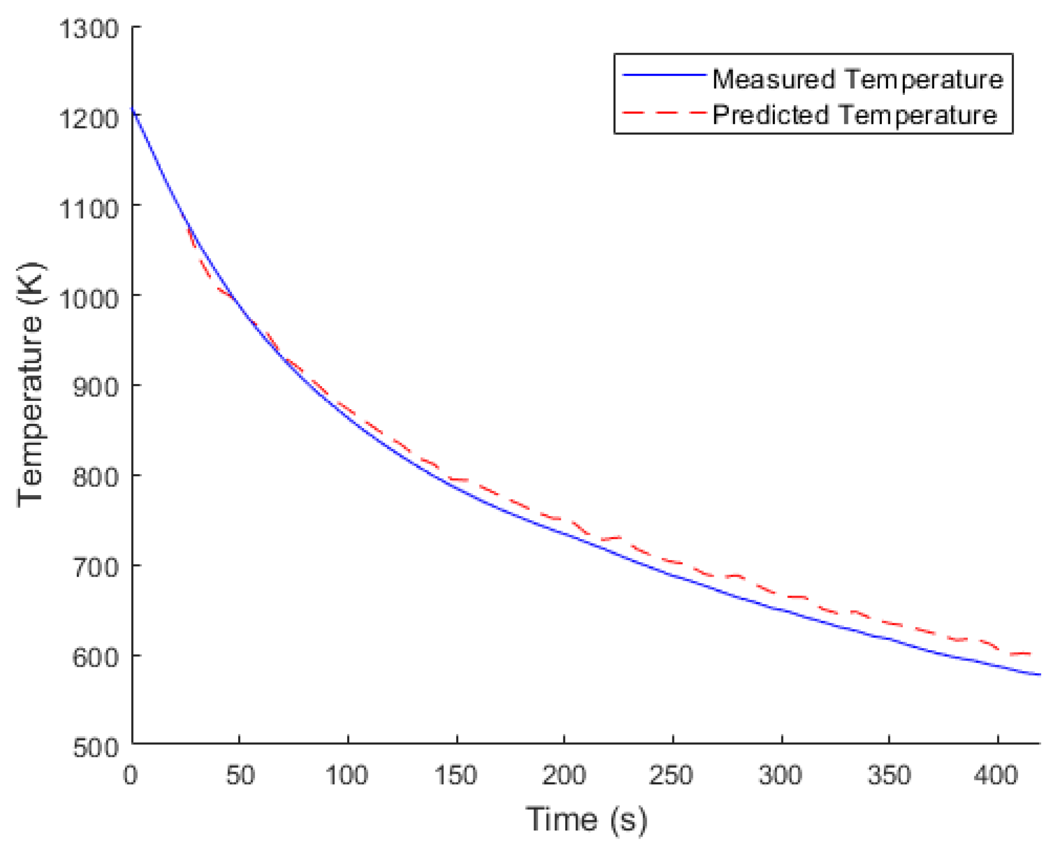
Figure 5 shows the measured temperature of the test rod in the test setup as it cools from 1150 K as well as the predicted temperature from the support vector regression model. Because the first 300 s are used for training, the model’s results only begin to diverge after that initial training period; however, the predicted temperature closely matches the measured temperature over the entire cooling period, only reaching a maximum error of
. This shows the method is adequate in predicting a single rod temperature in a simple geometry, and can be tested on more complicated rod bundle geometries.
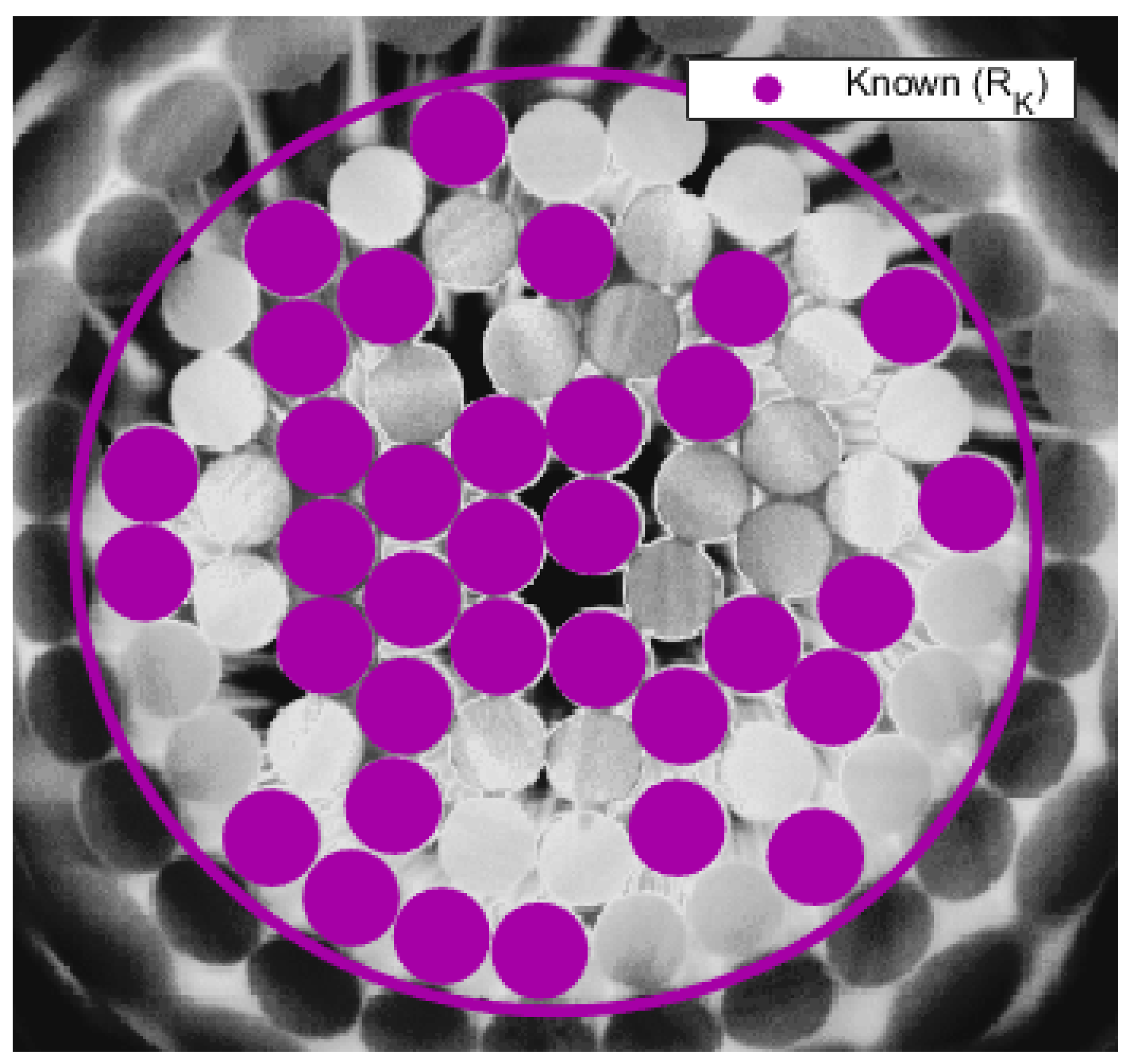
To analyze the SVR method with a more complex geometry, a randomly packed assembly of 68 rods was placed in the process tube and heated to a uniform temperature of approximately 1200 K. An IR camera was used to record the temperatures of each rod as the randomly packed rod assembly was allowed to cool to ambience. The training dataset consisted of the temperatures for all rods for the first 30 s and the temperatures for 34 randomly selected rods over the entire time domain.
Figure 6 shows the locations of the 34 randomly selected rods where the temperatures are known over the entire time domain. The values of parameters used in both regression models are shown in
Table 2. These locations are intended to mimic the locations of working temperature sensors in a reactor core. The test dataset consists of the temperatures for the remaining 34 rods over the time domain after
s. These rods are intended to mimic the locations in a reactor core where there are missing or inoperable temperature sensors. The training dataset is inputted into the model to predict the temperatures of these rods, and then compared with the measured temperatures.
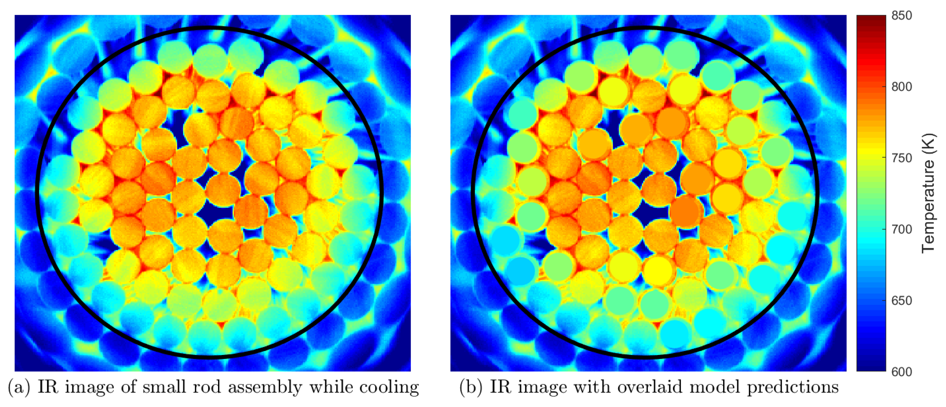
Figure 7a shows a temperature map of the 68 rod assembly at
s.
Figure 7b shows the same temperature map with the model predicted temperatures overlaid for the 34 rods in the test set. At this point in time, the model shows good agreement with the measured temperature values.
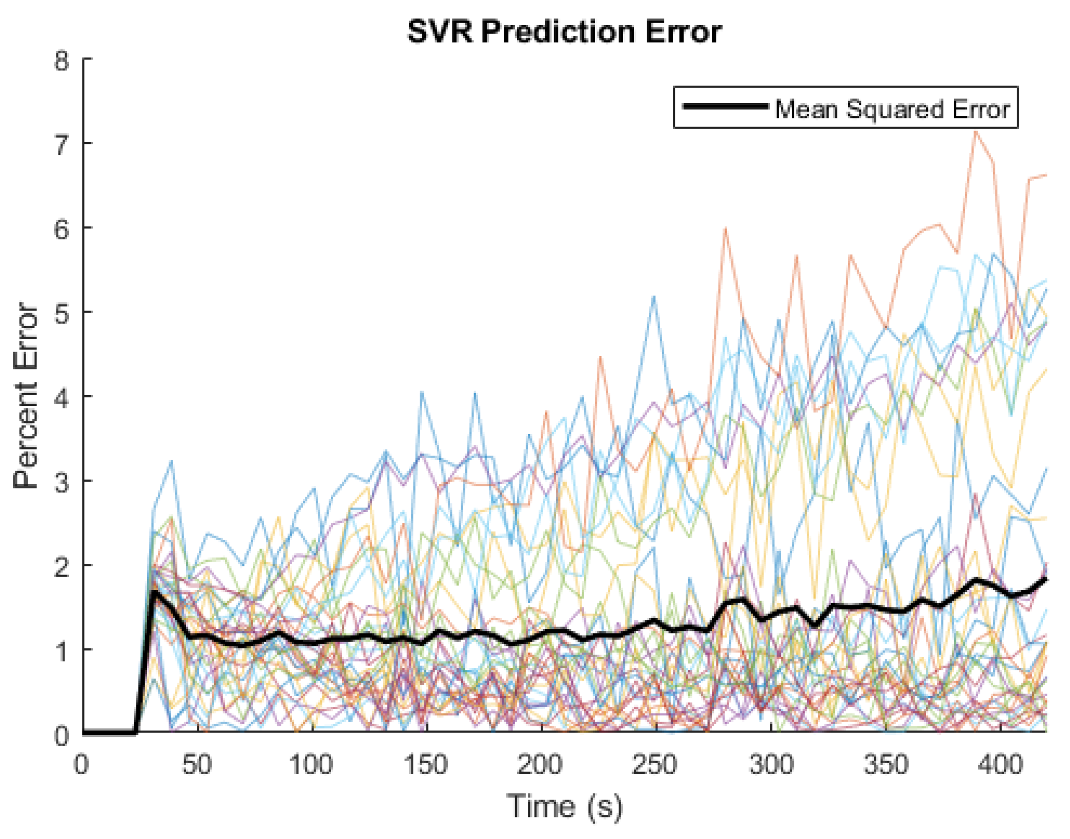
Figure 8 shows a comparison of the rod temperature over time for the rod with the greatest relative error, where the measured temperature is shown in blue and the temperature predicted with the SVR method is shown in red. As a whole, the predicted temperatures show no major deviation from the measured temperatures. The normalized error for each rod,
i, at time,
t, is defined as:
The error over time for each rod is shown in
Figure 9, with the mean squared error in black. The error is negligent in the first 30 s, as the temperatures are known for all rods and are used to train the regression model. The error jumps to approximately
in the first 25 s after
as the predicted temperature deviates from the calibrated training data and begins using the regression model. The error then levels off over the remaining time; however, there is a slight increase in the error as time progresses. This is to be expected, as this model only takes into account the connectivity of rods and their temperatures over time. As the cooling process progresses over time, heat transfer coefficients change, meaning there will be some variation in the thermal coupling both between the rods themselves and between the rods and the surroundings. The SVR model does not account for these thermal changes, so it is completely reliant on current and previous temperature values and their thermal connectivity, which are likely to change slightly over time.
Through the entire time domain, the average error stayed below
and the maximum error for any rod stayed below
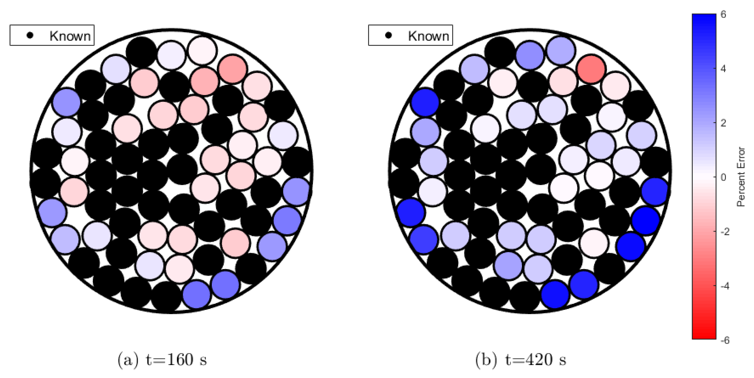
. Although maximum error reaches 7%, this is only observed when all the rods have cooled down below 600 K. Error increases for some rods as the assembly reaches lower temperatures because radiation losses to ambience reduce considerably. However, the prediction error was not consistent across the spatial domain. Throughout the entire cooling time, the prediction error for rods on the outside ring of the rod assembly had significantly higher error than those on the interior, indicating that the SVR model is better for interior rods and worse for exterior rods.
Figure 10 shows a map of the rod assembly with the time-averaged percent error for each rod. Rods in the training set where the temperatures are known in the model, as well as the exterior process tube, are indicated in black. For the rods whose temperatures are predicted using the SVR algorithm, the largest positive error (over-predicted) is indicated with a dark blue, and the largest negative error (under-predicted) is indicated with dark red. As is shown, all of the rods with the highest error are in the outer ring of the rod assembly, while all the rods with the lowest error are on the interior. Rods which are contacting the process tube are also more likely to have higher error than those on the exterior which do not contact the process tube. This is likely due to the non-constant effects of the heat transfer properties from the process tube to the environment, while the SVR model includes a node to model the connection to the process tube and surroundings, this single node is likely not enough to model the complexity of heat transfer through the process tube and surrounding environment. For horizontally oriented reactor cores, the heat removal rate to the surroundings is likely to vary azimuthally, meaning that the heat transfer rates for rods contacting the bottom of the process tube could vary significantly from the heat transfer rate for rods contacting the top of the process tube. This error, while small, could be magnified by a more complex heat removal process at the boundary of the rod assembly than the one presented in this work.
5. Conclusions
Previous incidents at nuclear power facilities made it clear that even with rigorous safety procedures and in-depth computer models, it is difficult to predict or control the progression of off-normal events impacting nuclear power plants. Inherently safe reactors with passive cooldown capabilities are essential for the future of nuclear energy around the world. One way to improve safety in advanced reactors while keeping autonomous operation is by using sensors and machine learning effectively. These data model-based projections will not only be critical for enhancing safety, but will also aid in reducing O&M costs by enabling autonomously controlled safety systems. Two high-temperature conduction cooldown experiments were performed, the first using 7 alumina rods and the second using 68 graphite rods. Thermographic images were obtained and used to record the temperatures of the rods to serve as both validation for the predicted values as well as training data for the model. This machine learning technique was devised to construct the thermal response of the entire domain using discrete random sensor data under conduction cooldown experiments. Initial tests with the seven-rod setup proved that the method was capable of providing accurate predictions with a maximum error of . For the second set up, with knowledge of the temperature data for 34 rods in a randomly packed assembly, the temperatures of the remaining 34 rods could be accurately predicted over 400 s with an average accuracy within .
The accuracy of the model was significantly better for the rods in the interior of the assembly over the rods in the outer ring. This is likely due to the uncertainty of heat transfer properties and their impact on the heat removal from the core to the surroundings. Future work will involve changing the model to better represent the external convection as well as extending this approach to 3D spherical pebble beds and prismatic block geometries with decay heat generation, which are more common HTGR designs.
Author Contributions
Conceptualization, D.G., S.D. and H.B.; Data curation, M.R., T.-Y.L. and D.G.; Funding acquisition, H.B.; Supervision, S.D. and H.B.; Validation, H.B.; Visualization, M.R. and T.-Y.L.; Writing—original draft, D.G., S.D. and H.B.; Writing—review and editing, H.B. All authors have read and agreed to the published version of the manuscript.
Funding
This research is supported by Department of Energy NEUP program.
Institutional Review Board Statement
Not applicable.
Informed Consent Statement
Not applicable.
Data Availability Statement
Available upon request.
Conflicts of Interest
The authors declare no conflict of interest.
References
- Patterson, E.A.; Taylor, R.J.; Bankhead, M. A framework for an integrated nuclear digital environment. Prog. Nucl. Energy 2016, 87, 97–103. [Google Scholar] [CrossRef]
- Kochunas, B.; Huan, X. Digital twin concepts with uncertainty for nuclear power applications. Energies 2021, 14, 4235. [Google Scholar] [CrossRef]
- Grieves, M.; Vickers, J. Digital twin: Mitigating unpredictable, undesirable emergent behavior in complex systems. In Transdisciplinary Perspectives on Complex Systems; Springer: Berlin/Heidelberg, Germany, 2017; pp. 85–113. [Google Scholar]
- Cortés, O.; Urquiza, G.; Hernandez, J.; Cruz, M.A. Artificial neural networks for inverse heat transfer problems. In Proceedings of the Electronics, Robotics and Automotive Mechanics Conference (CERMA 2007), Morelos, Mexico, 25–28 September 2007; pp. 198–201. [Google Scholar]
- Goudarzi, K.; Moosaei, A.; Gharaati, M. Applying artificial neural networks (ANN) to the estimation of thermal contact conductance in the exhaust valve of internal combustion engine. Appl. Therm. Eng. 2015, 87, 688–697. [Google Scholar] [CrossRef]
- Yovanovich, M.M. Four decades of research on thermal contact, gap, and joint resistance in microelectronics. IEEE Trans. Components Packag. Technol. 2005, 28, 182–206. [Google Scholar] [CrossRef]
- Xu, R.; Feng, H.; Zhao, L.; Xu, L. Experimental investigation of thermal contact conductance at low temperature based on fractal description. Int. Commun. Heat Mass Transf. 2006, 33, 811–818. [Google Scholar] [CrossRef]
- Gould, D.W.; Bindra, H.; Das, S. Thermal response construction in randomly packed solids with graph theoretic support vector regression. Int. J. Heat Mass Transf. 2017, 115, 421–429. [Google Scholar] [CrossRef]
- Filtz, J.; Lièvre, M.; Valin, T.; Hameury, J.; Wetterlund, I.; Persson, B.; Andersson, P.; Jansson, R.; Lemaire, T.; Öhlin, M.; et al. Improving Heat Flux Meter Calibration for Fire Testing Laboratories (HFCAL). Final Report; NordTest Technical Reports: Brussels, Belgium, 2002. [Google Scholar]
- Fouss, F.; Francoisse, K.; Yen, L.; Pirotte, A.; Saerens, M. An experimental investigation of kernels on graphs for collaborative recommendation and semisupervised classification. Neural Netw. 2012, 31, 53–72. [Google Scholar] [CrossRef] [PubMed]
- Smola, A.J.; Kondor, R. Kernels and regularization on graphs. In Learning Theory and Kernel Machines; Springer: Berlin/Heidelberg, Germany, 2003; pp. 144–158. [Google Scholar]
- Basak, D.; Pal, S.; Patranabis, D. Support Vector Regression. Neural Inf. Process.—Lett. Rev. 2007, 11, 203–224. [Google Scholar]
| Publisher’s Note: MDPI stays neutral with regard to jurisdictional claims in published maps and institutional affiliations. |
© 2022 by the authors. Licensee MDPI, Basel, Switzerland. This article is an open access article distributed under the terms and conditions of the Creative Commons Attribution (CC BY) license (https://creativecommons.org/licenses/by/4.0/).


