
CTF-PARCS Core Multi-Physics Computational Framework for Efficient LWR Steady-State, Depletion and Transient Uncertainty Quantification

 , , , , and
Abstract
:1. Introduction
2. Computational Framework
2.1. Simulation Tools
2.1.1. Polaris
2.1.2. Sampler
2.1.3. GenPMAXS
- The configuration of the fuel or reflector assembly defined by the assembly specifications, such as the pin pitch, number of pin per assembly. Those specifications are required in the PMAXS for pin power reconstructions.
- The cross-section parameterization (branch, history, burnup). GenPMAXS also requires the definition of a reference history and branch.
- Pre-defined user inputs. For example, the name given to the PMAXS file, boolean flags such as inclusion of assembly and axial discontinuity factors.
2.1.4. PARCS
2.1.5. CTF
2.1.6. Dakota
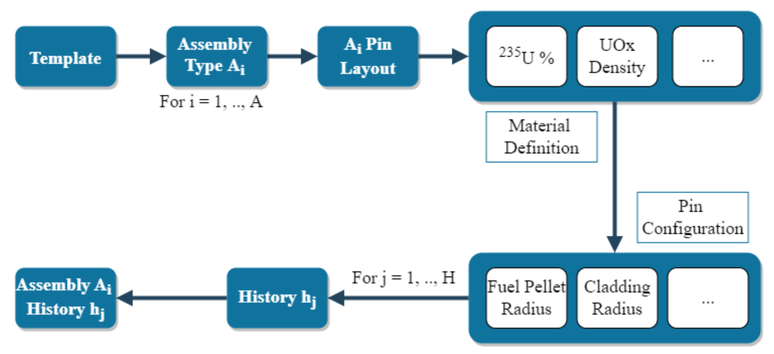
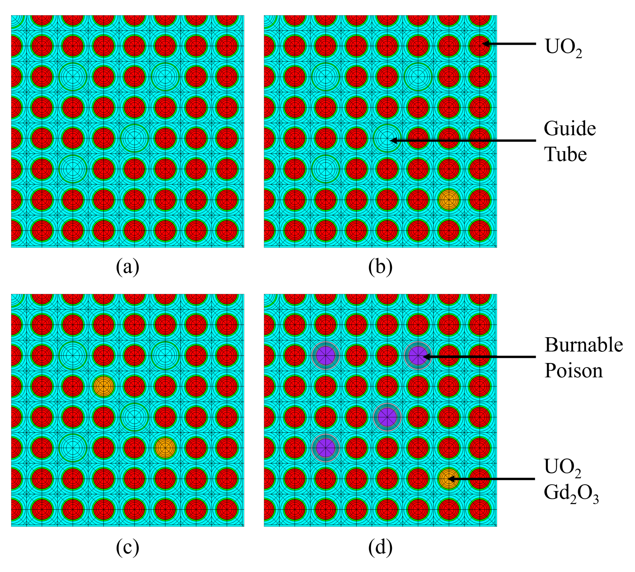
2.2. Polaris Pre-Processing
- The pin layout.
- The material definitions.
- The reference state.
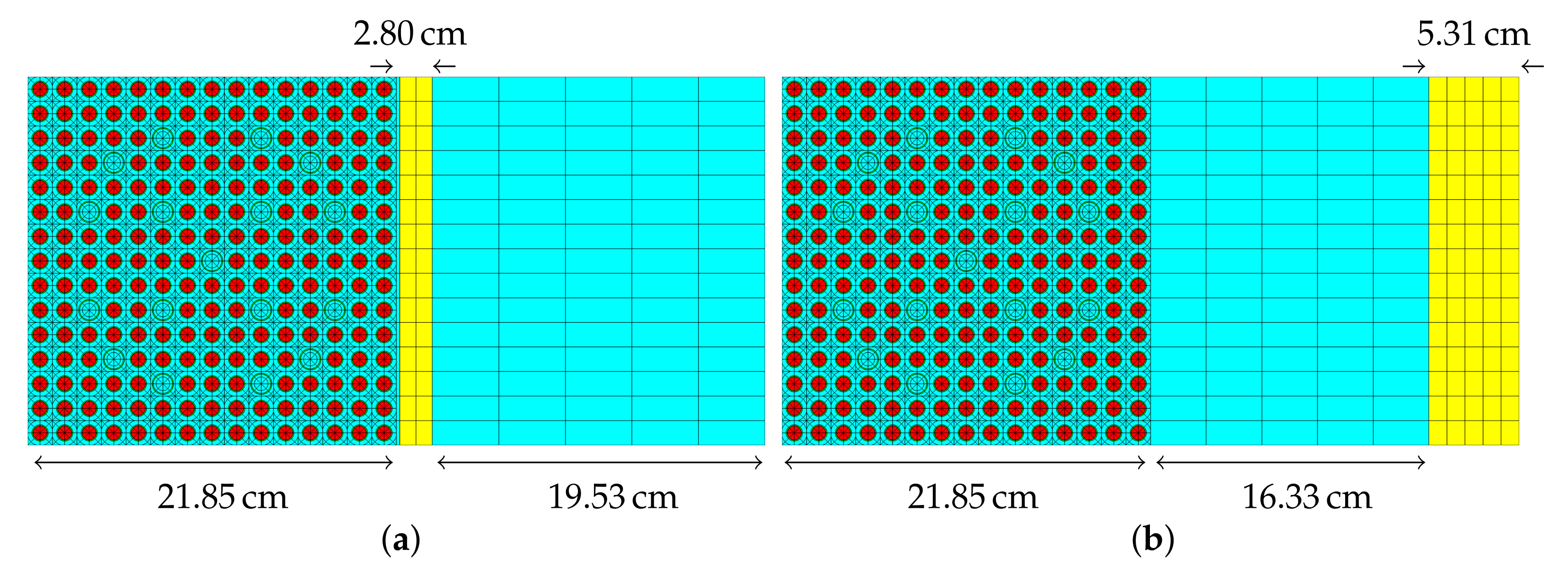
- The core plate thickness or shroud thickness, if any, for reflector assemblies.
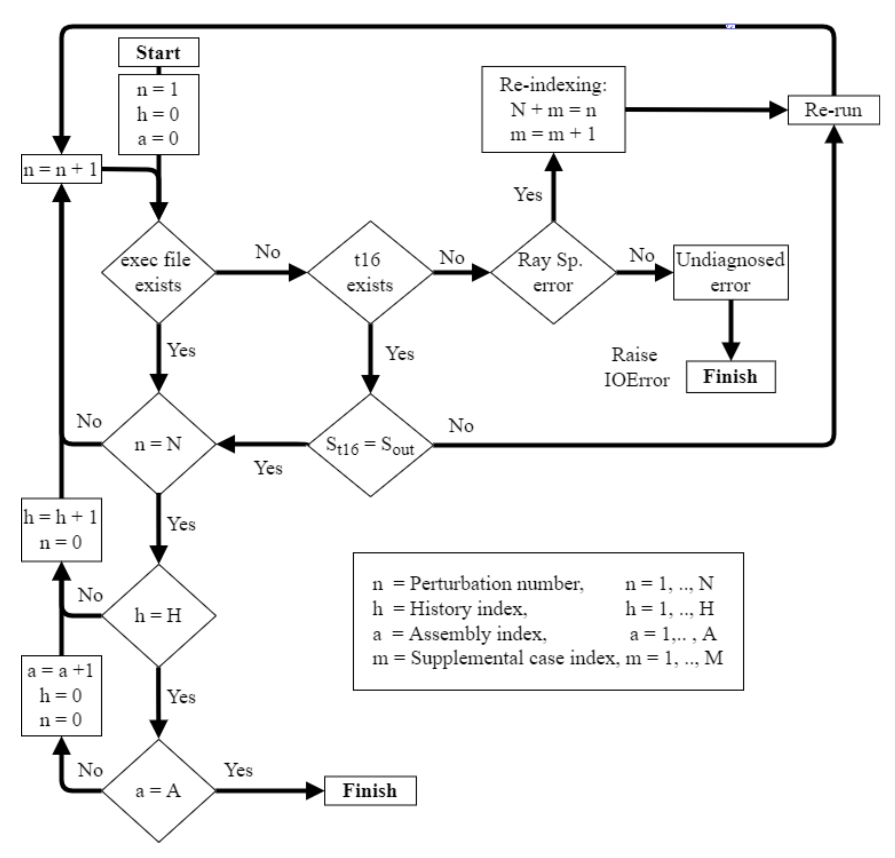
- If a SCALE execution file exists ( file), the job is currently running, and the sequence moves on to the next perturbation, .
- If no file and no Polaris output () exist, the perturbation case has not been run yet: the sequence runs the simulation normally and moves on to the next perturbation, .
- If the file and Polaris output file both exist, the number of state points computed in the file () is cross-compared to the expected number of state points predicted by the Polaris output ().
- -
- If = , the perturbation case has already run normally, and the sequence moves on to the next perturbations, .
- -
- Otherwise, the sequence raises an error, and no diagnostic is predicted.
- If the Polaris output exists, but the does not, the Polaris output is read by the sequence to find out if the simulation stopped due to a ray spacing error.
- -
- If a ray spacing error occurred, another perturbation is drawn from the supplemental inputs. The supplemental case indexed is re-indexed into , the case is re-run, and then the sequence moves on to the next perturbations, .
- -
- Otherwise, a job crash is assumed (exceeded wall time, reboot, etc.) and the perturbation is re-run without modification and then moves onto the next perturbation, .
2.3. CTF-PARCS Coupling
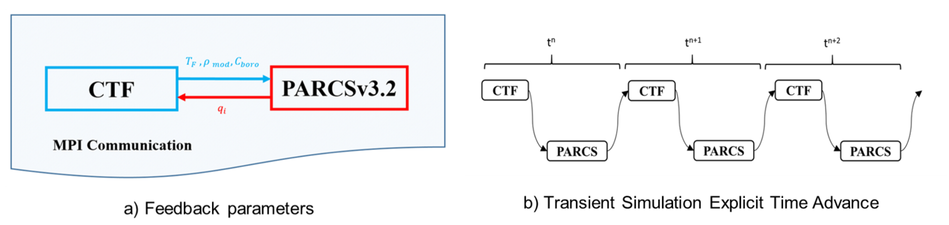
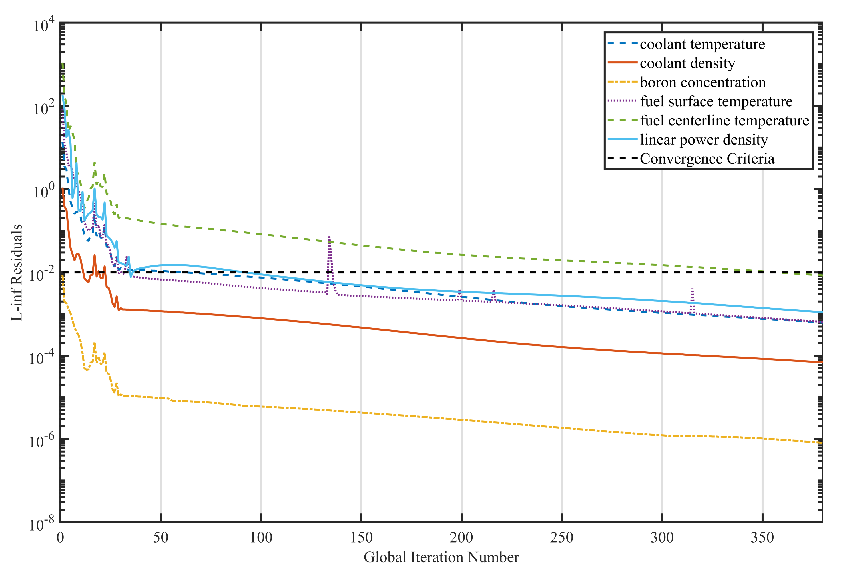
- In steady-state mode, a simple Picard iteration scheme [14] has been adopted. This method implies the construction of an outer convergence loop to check for global convergence of the coupled code and as many local convergence loops as physics are being coupled together. These nested loops represent the global coupled convergence. In this method, the convergence of the thermal-hydraulic code has to be fully met before providing feedback to the neutronic code. The neutronic code then uses the thermal-hydraulic feedback to resolve the neutron flux distribution until its own convergence criteria are met. The global coupled code convergence is tracked by the residuals of the feedback parameters using the and norms of each parameter until the defined tolerance is reached. The and norms are defined in Equations (3) and (4), respectively, where is the cell number, is the total number of cells, is the index of the residual of a given feedback parameter, and is the total number of residuals. is the residual of the feedback parameter in the cell for the current iteration, which is computed as , among which is the current iteration number. The coupled code steady-state convergence behavior is illustrated in Figure 6.
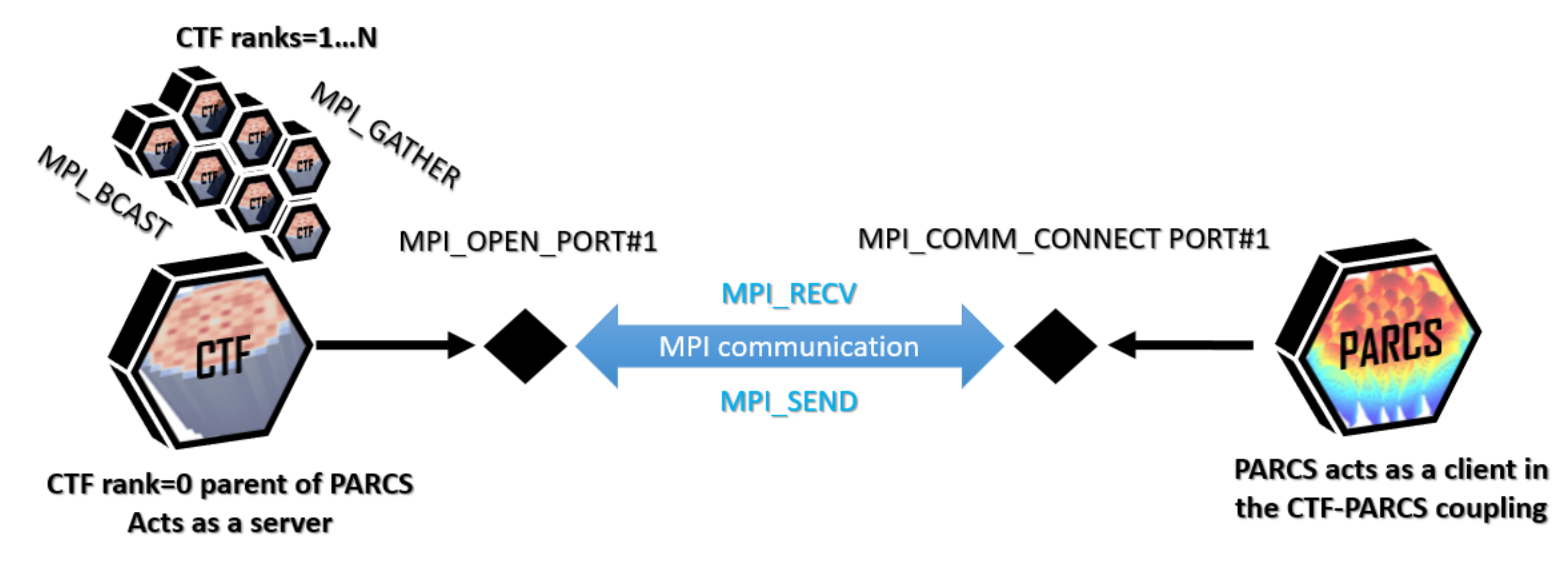
- For transient simulations, a temporally explicit coupling scheme has been adopted. Therefore, the neutronic and thermal-hydraulic conservation equations are not solved altogether, but each code solves its own system of transient equations using the most limiting time step size of both codes. This explicit client/server coupling scheme is presented in Figure 5b. The temporally explicit methods are usually adopted when coupling thermal-hydraulics with neutron kinetics because the numerical stability is always preserved. Although it is widely adopted, the temporally explicit coupled methods have two main inconveniences. The first issue is the numerical diffusion, as each of the coupled physics relies on the solution of the other physics at the previous time step. The second inconvenience is the limitation of the time step size, as all the coupled codes must adopt the smaller time step size between all the involved physics.
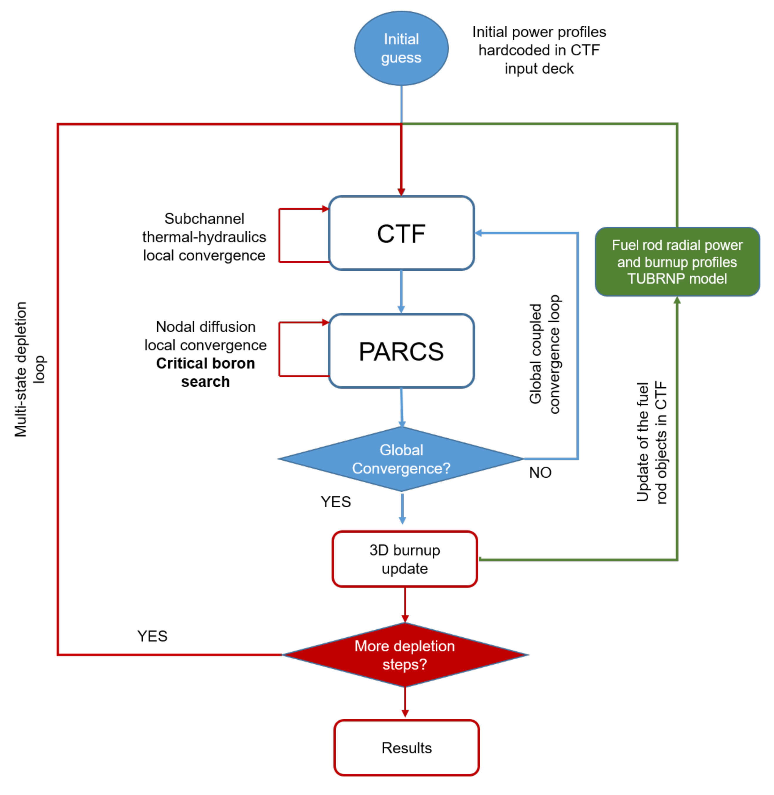
- In depletion mode, a multi-state simulation procedure is initialized in the core simulator. The number of states of this multi-state mode is defined by the number of depletion steps set in PARCS input. At the beginning of each state, the 3D burnup distribution is sent from PARCS to CTF to initialize the burnup-dependent models and material properties in the fuel rod objects. After this initialization, the Picard iteration global convergence scheme is used in the same way as in steady-state simulations. It must be noted that the boron concentration is not feedbacked from CTF to PARCS in depletion mode, as the critical boron is the parameter varied by the latter to find the criticality of the core. This multi-state iterative procedure is represented in the scheme of Figure 7. The global convergence of the developed core simulator in depletion mode can be analyzed by looking at the norms presented in Figure 8. In Figure 8, it can be observed that the global convergence is longer in the first iteration because the initial conditions are far from the real solution. All the remaining states converge with a similar convergence ratio. Each peak on the residual represents the beginning of each state. The peaks are large due to the change in the 3D burnup distribution in the core.
- The first development is the possibility of defining customized ways to compute the Doppler fuel temperature. This effective fuel temperature can be defined as a linear combination of the pellet radial average temperature (), the fuel surface temperature (), and the fuel centerline temperature (), as shown in Equation (5). The parameters , , and are defined by the user in the coupling interface input file.This allows the user complete flexibility on the definition of the effective temperature. Typical effective fuel temperature formulas found in the literature that can be reproduced with this development are the Rowlands [33], as shown in Equation (6), and the Santamarina [34], as shown in Equation (7).
- The second added feature is the initialization of the pellet power and exposure radial profiles in CTF. This capability has been implemented by linking an external 1D depletion module to CTF. This external depletion module can be called from the fuel rod class of CTF to make a depletion and obtain the radial power and exposure profiles for each nuclear rod and axial node of the model.
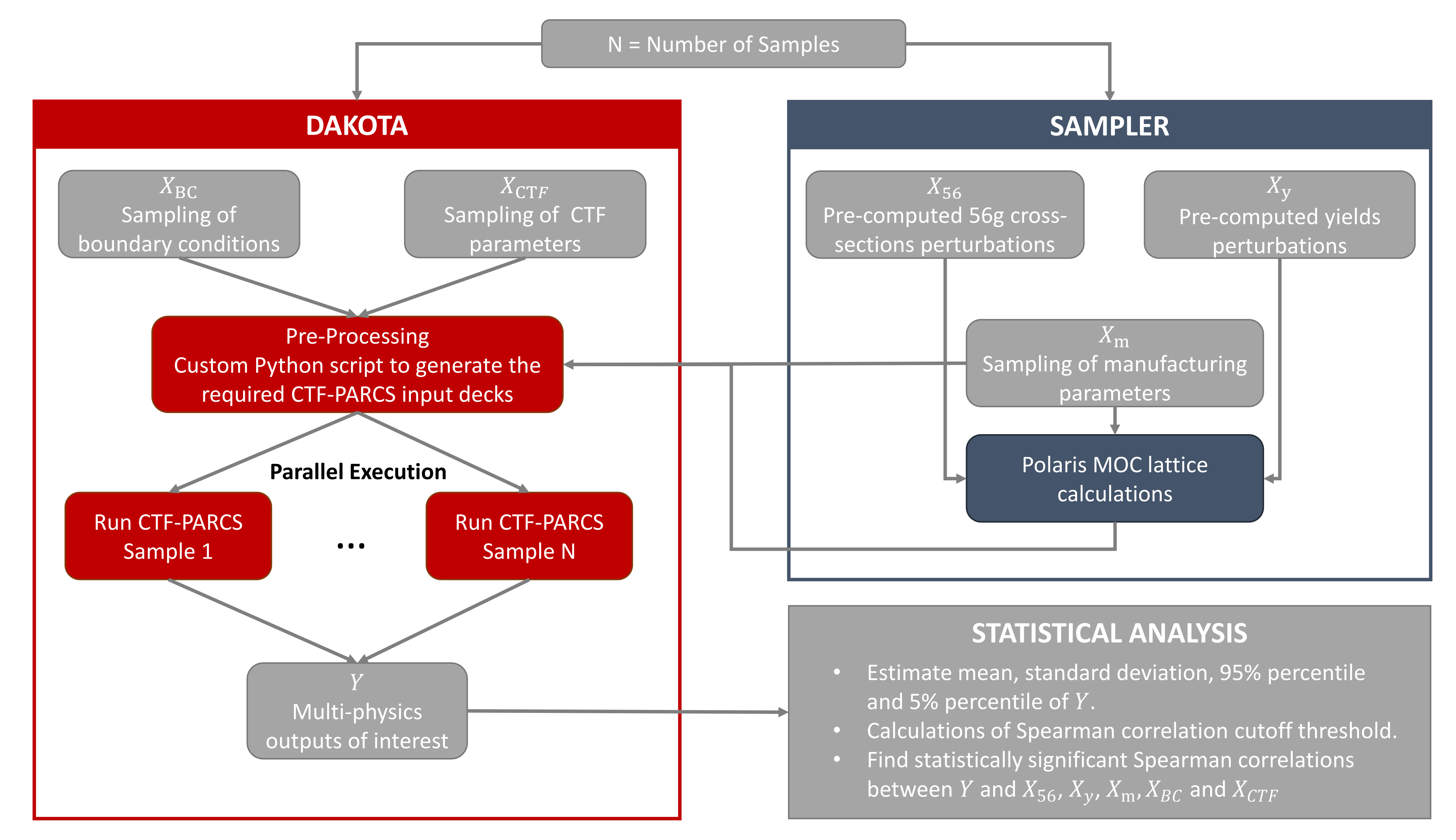
2.4. Uncertainty Quantification
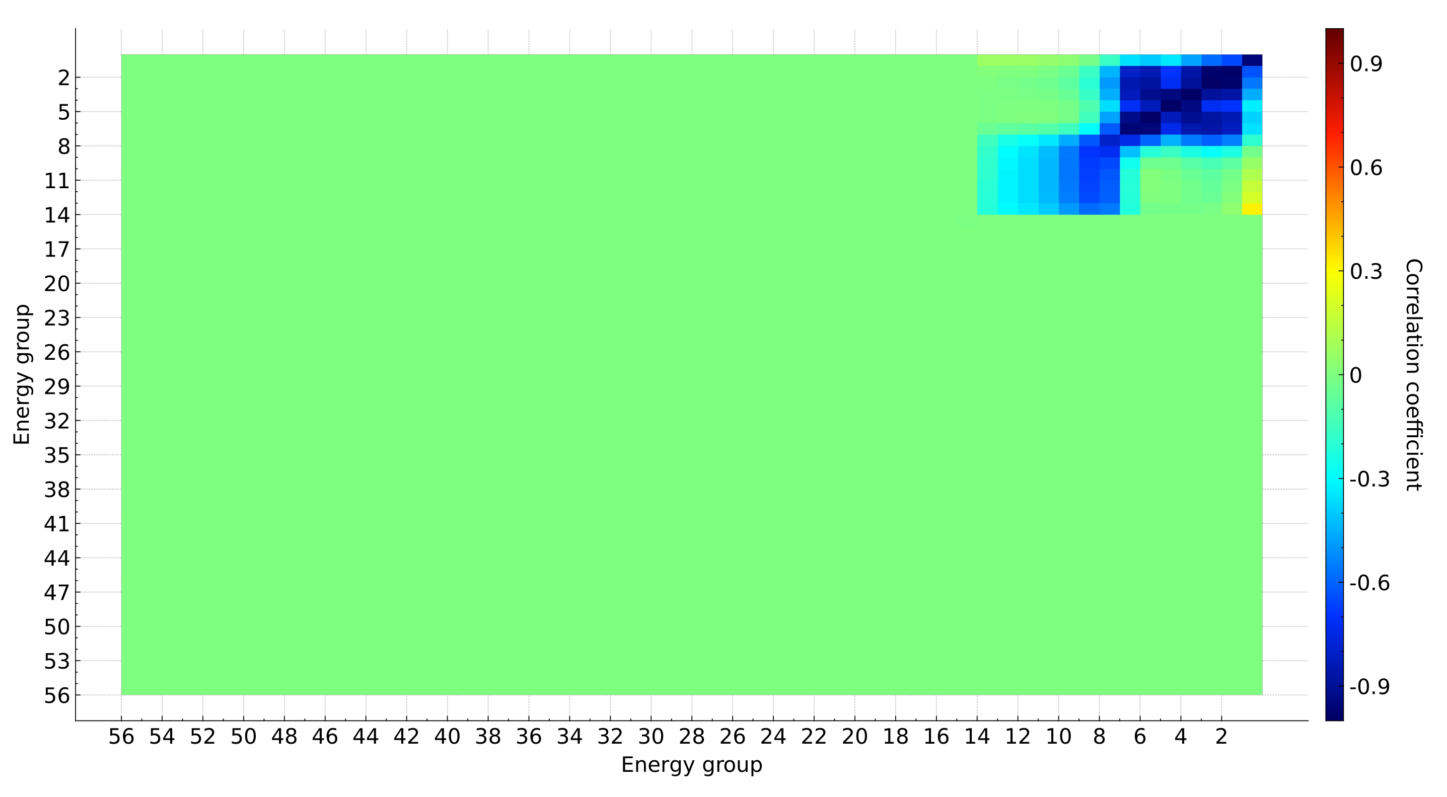
- The first aspect is the statistical noise. Due to the limited number of samples, even independent quantities can be correlated up to some degree. For this reason, a cutoff threshold needs to be determined in order to screen out all the correlations that are within the statistical noise. To calculate the cutoff threshold, a very simple brute force approach is performed. For a predefined number of iterations , in each iteration, two standard normal variables are sampled independently with the intended number of samples . The correlation between these two variables is then estimated and stored. This results in a vector of correlations of size that represents a distribution of empirically estimated correlations of independent variables and thus can be used to derive a cutoff based on some statistical measure. The percentile is considered in this work as the cutoff. As we are going to see later, samples were used, and the calculated cutoff threshold was found to be . This means that any correlation that, in absolute value, is larger than is considered as statistically significant. The cross-sections that show at least one group to be statistically significant are analyzed at all their energy groups, as shown in the uncertainty quantification results section, in order to better understand the energy dependence of the estimated correlations.
- The second aspect is the fact that if a very large number of inputs contribute approximately equally to the output, then it will be difficult to even distinguish them from the noise. This can be remedied by increasing the number of samples, since the cutoff threshold will decrease. Additionally, in most of the applications, few inputs contribute significantly more than the others, which facilitates their identification. The latter of course cannot be known in advance but only after performing the multi-physics calculations for the specific application.
- The third and most important aspect is that the estimated correlations do not imply causation; in other terms, if an input shows strong correlation with an output, it does not mean that it is actually responsible for the output’s uncertainty. For this reason, a subjective analysis of the correlation matrices together with the physics understanding and experience can help deduce whether an input is actually important or it has high correlation, because it is correlated to another input, which is the one that is actually important. In any case, even if there is no objective way for such a simple uncertainty quantification approach to assign sensitivities in the multi-physics context, the resulting correlations are still very valuable and can inform future experiments to reduce the corresponding input uncertainties or correlations with other inputs. Finally, an ultimate test for this approach would be to compare the identified microscopic cross-sections for a steady-state standalone neutronics study with the ones identified using a perturbation-based approach. The validation of this proposed approach is left for future work.
3. LWR-UAM Phase III Core Study
3.1. Case Studies
3.2. Modeling
- Consideration of 3D burnup distribution in the thermal calculations. The burnup impacts the thermal conductivity and thus the fuel temperature.
- Radial power and burnup distribution within the representative fuel pin thermal calculation. The TUBRNP model, typically used in fuel performance codes, was used to calculate the burnup and power profiles for each local mesh based on the burnup of the mesh.
- Exchange of the updated burnup distribution between PARCS and CTF in the depletion calculations.
- Use of Santamarina effective Doppler temperature.
4. Results
4.1. HFP BOC REA
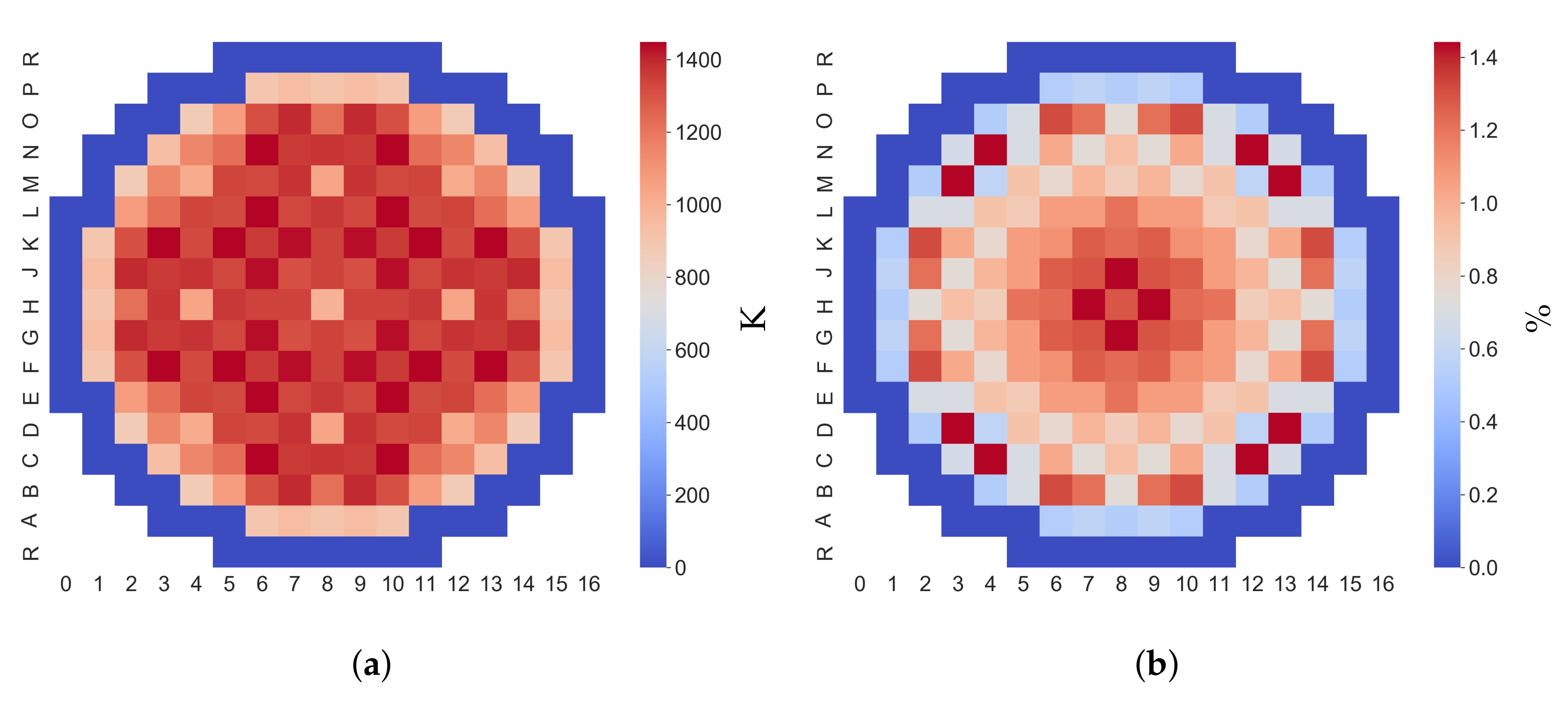
4.1.1. Steady State
- Fuel density: −0.39.
- Cladding inner radius: 0.75.
- Fuel thermal conductivity: −0.35.
- Gap conductance: −0.45.
- Mass flux: 0.46.
- Inlet temperature: −0.75.
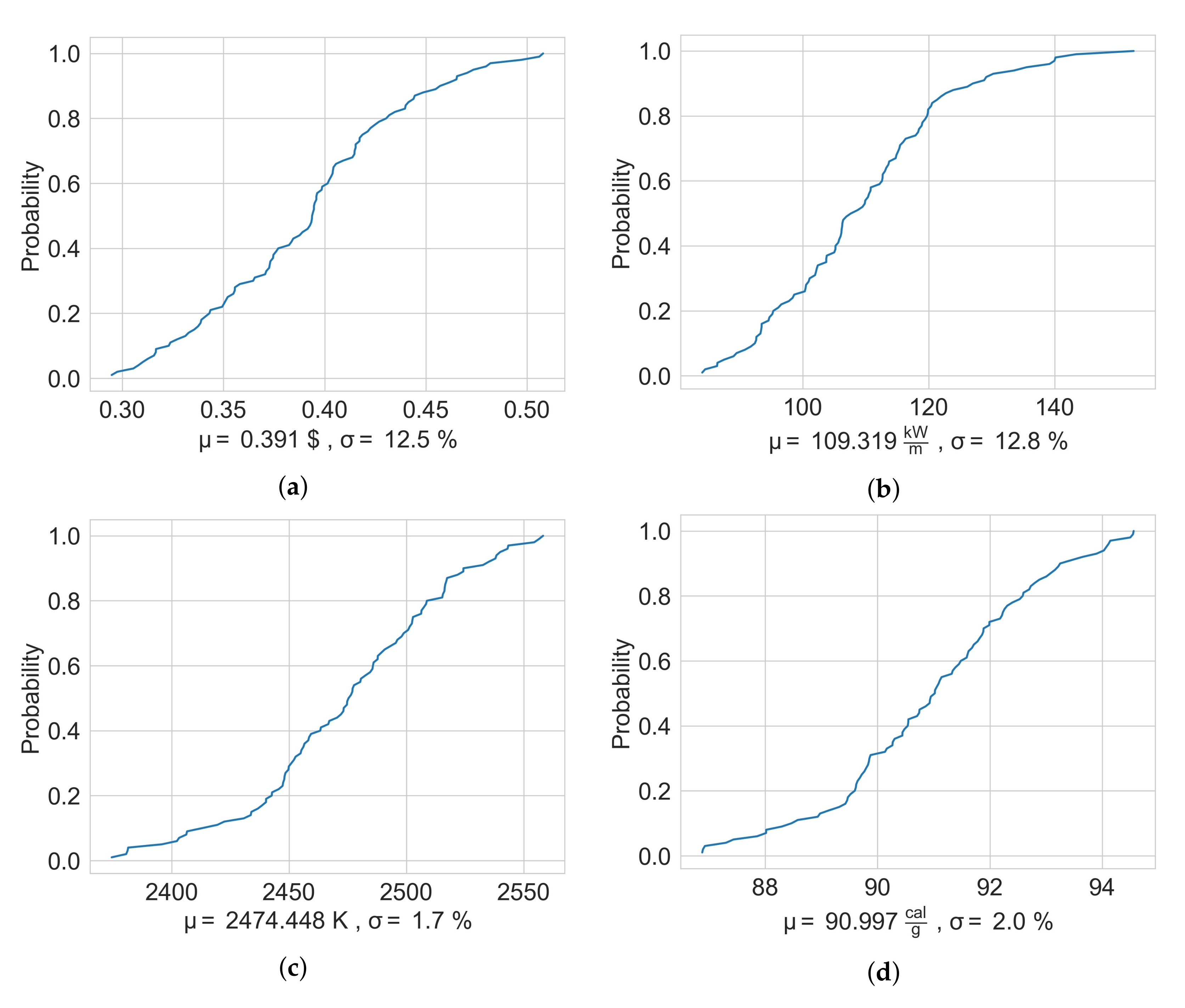
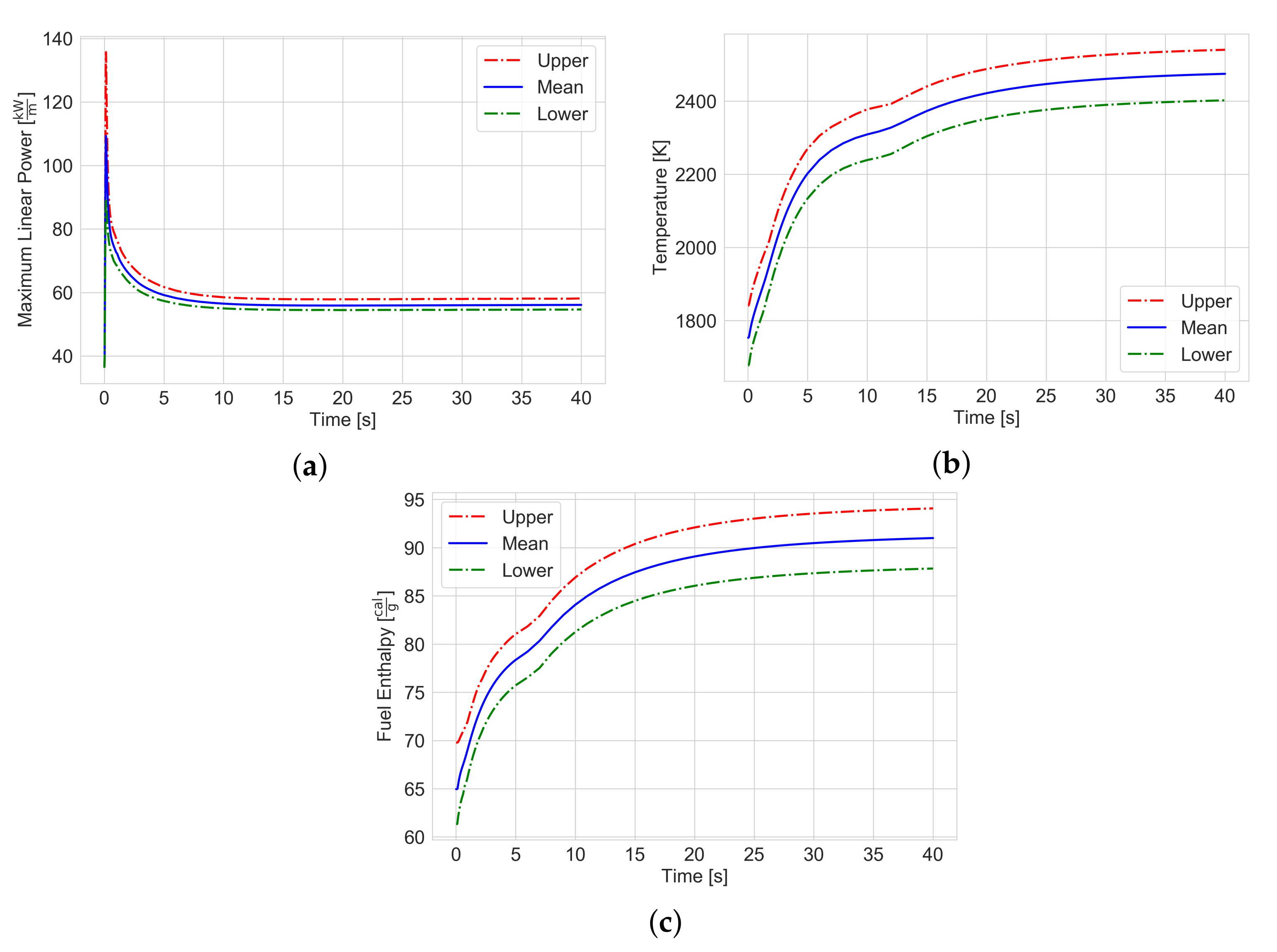
4.1.2. Transient
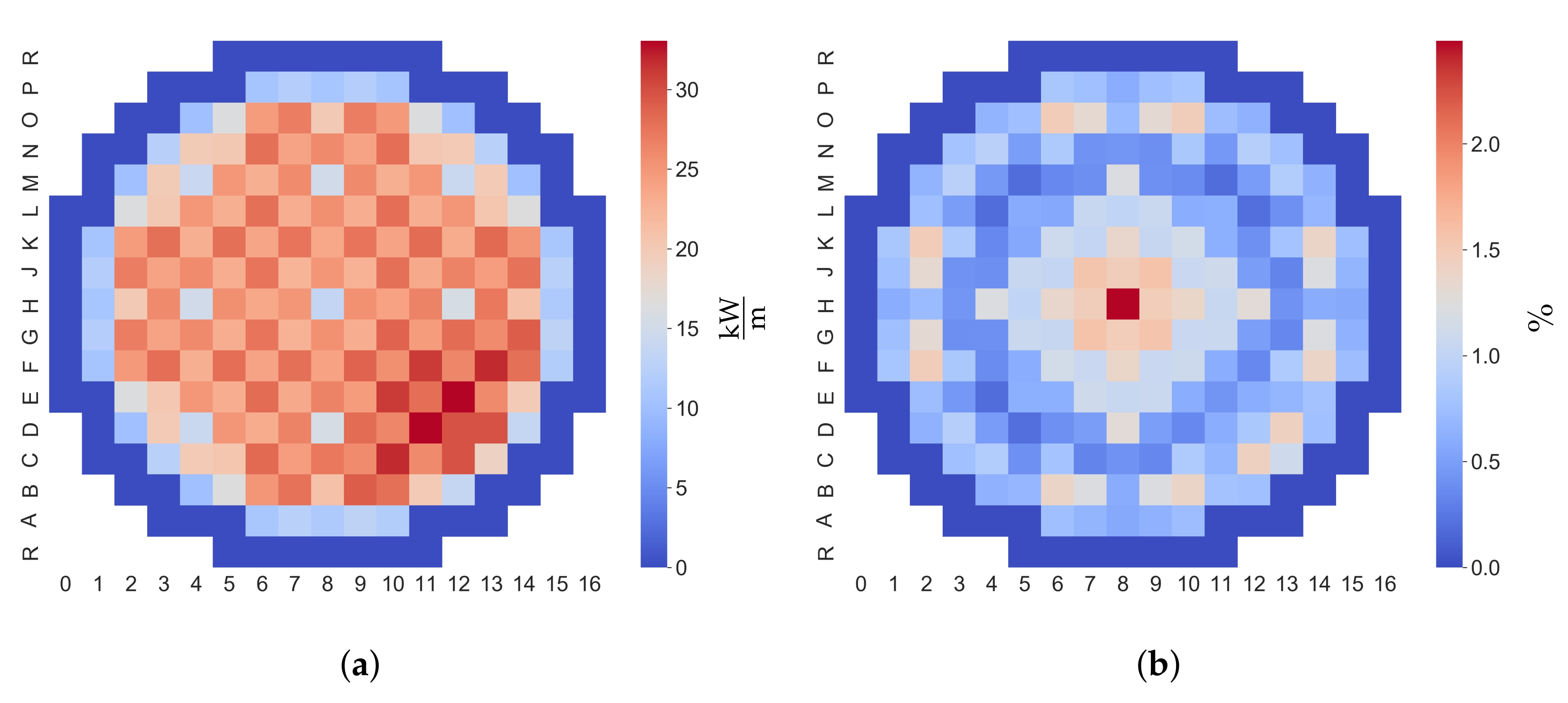
4.2. HFP EOC REA
4.2.1. Steady State
- Fuel density: −0.45.
- Fuel thermal conductivity: −0.46
- Mass flow rate: 0.41.
- Inlet temperature: −0.79.
4.2.2. Transient
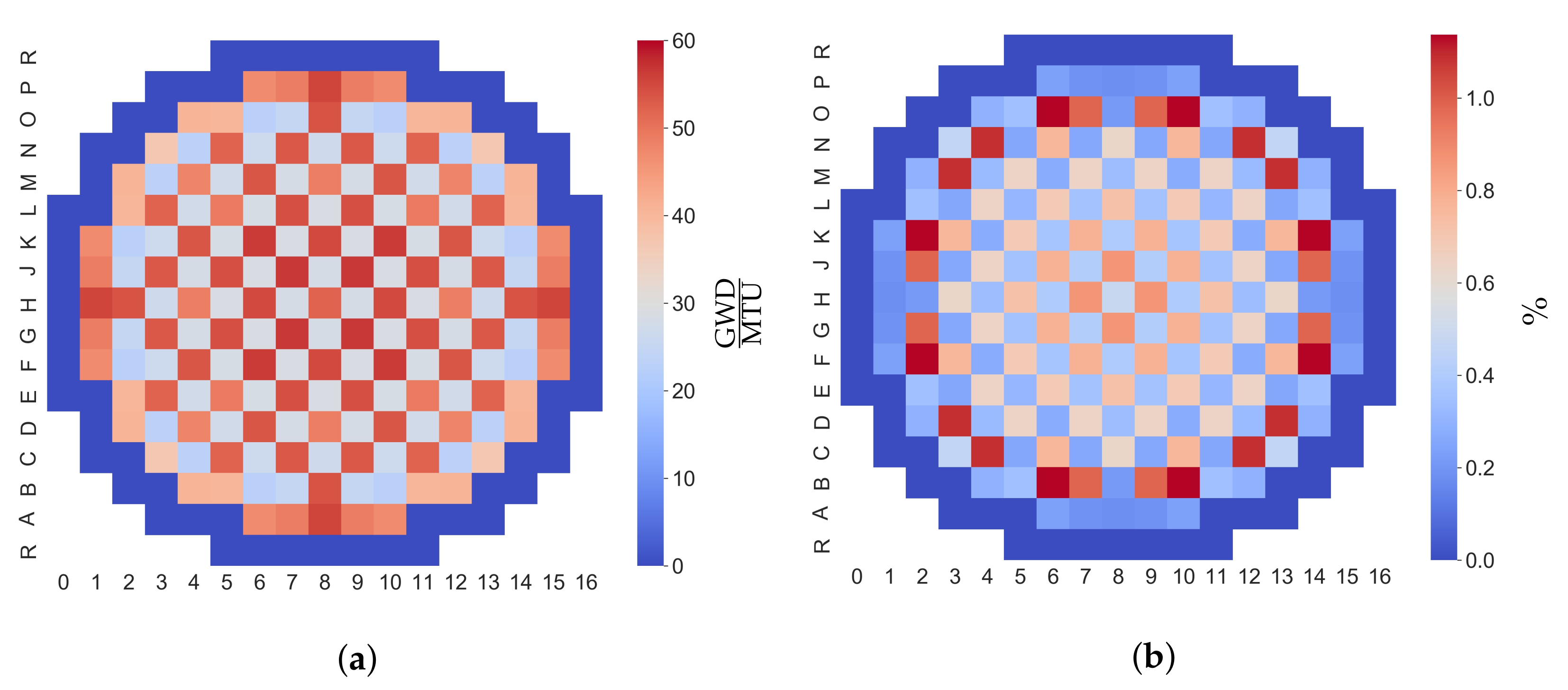
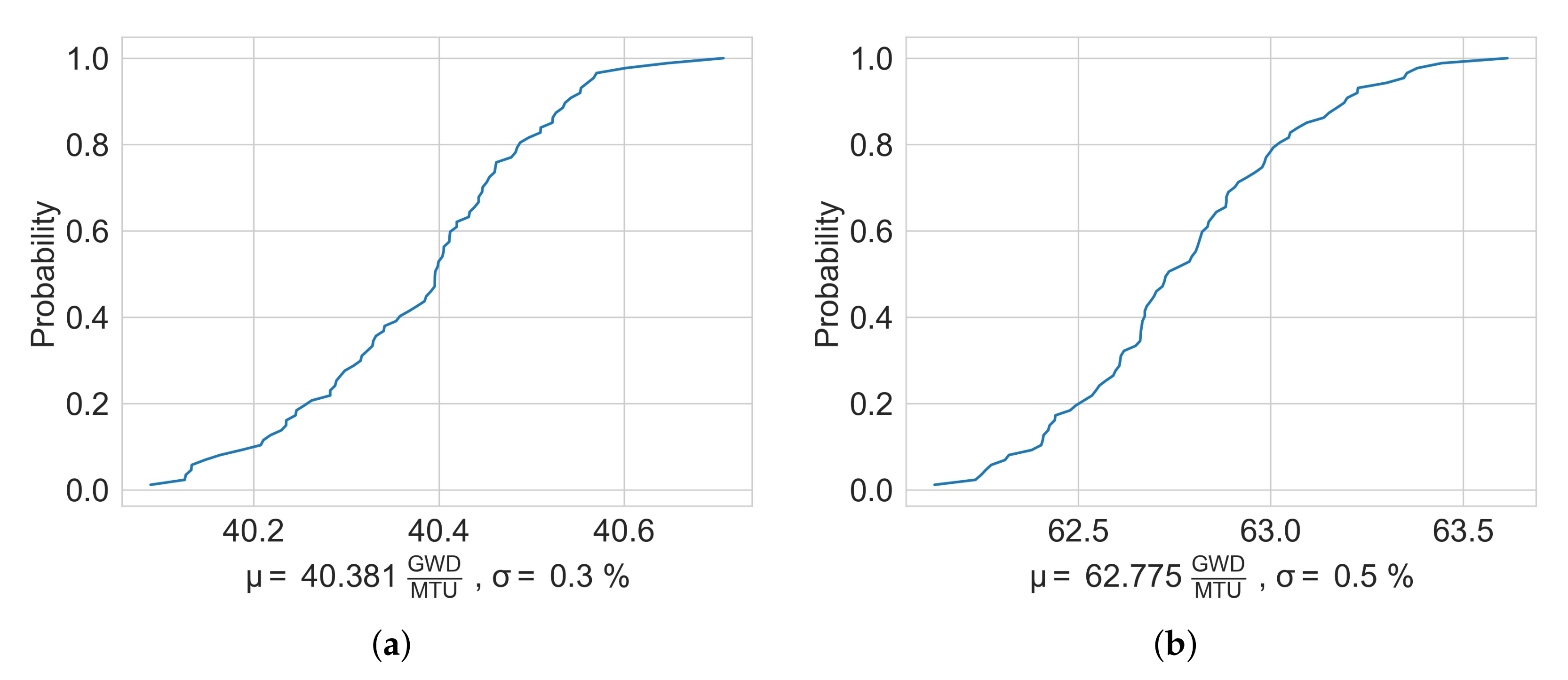
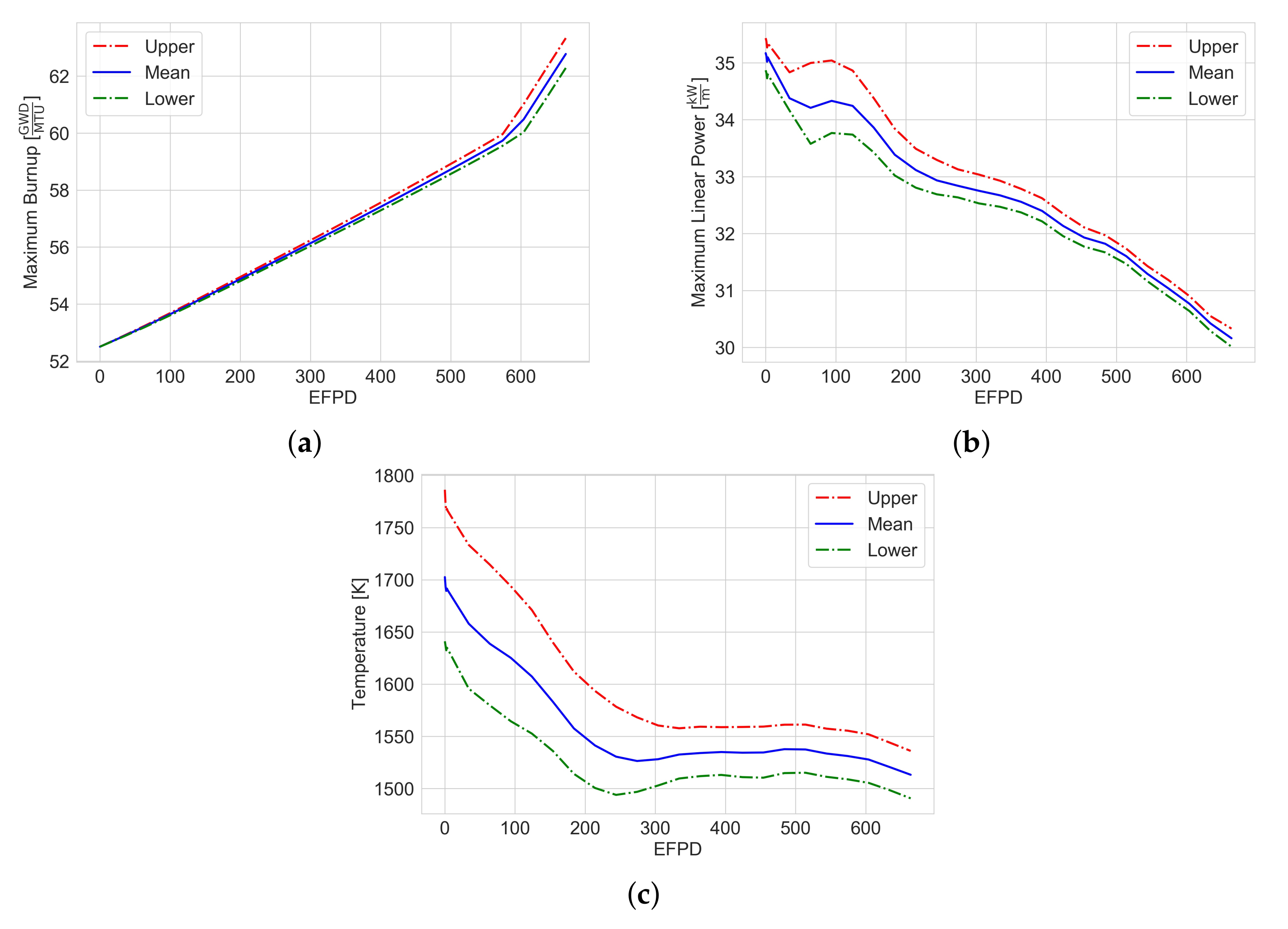
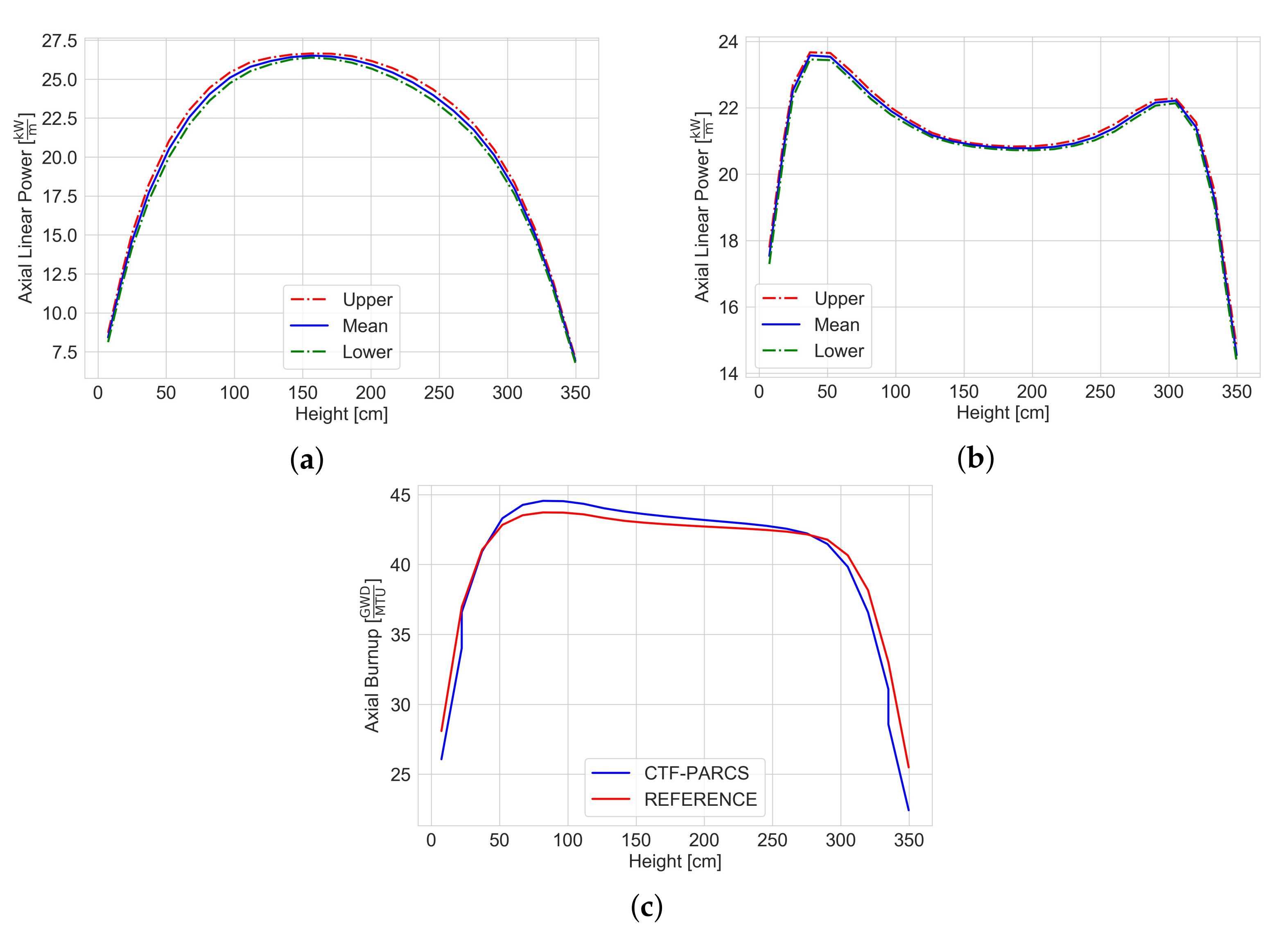
4.3. Depletion
5. Conclusions
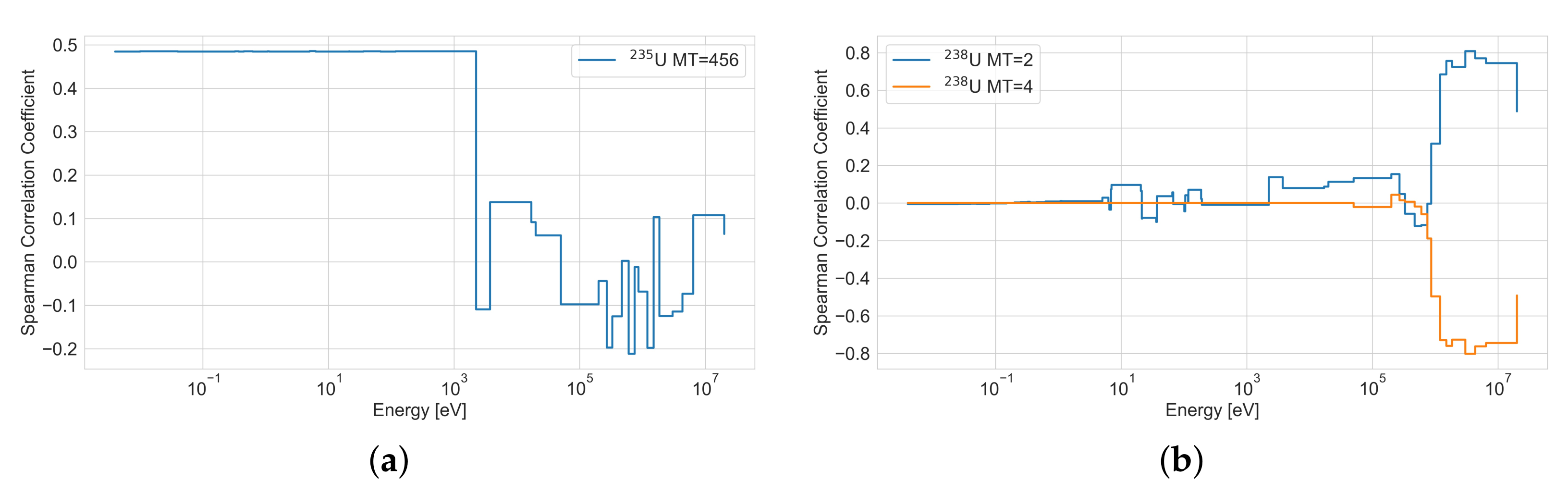
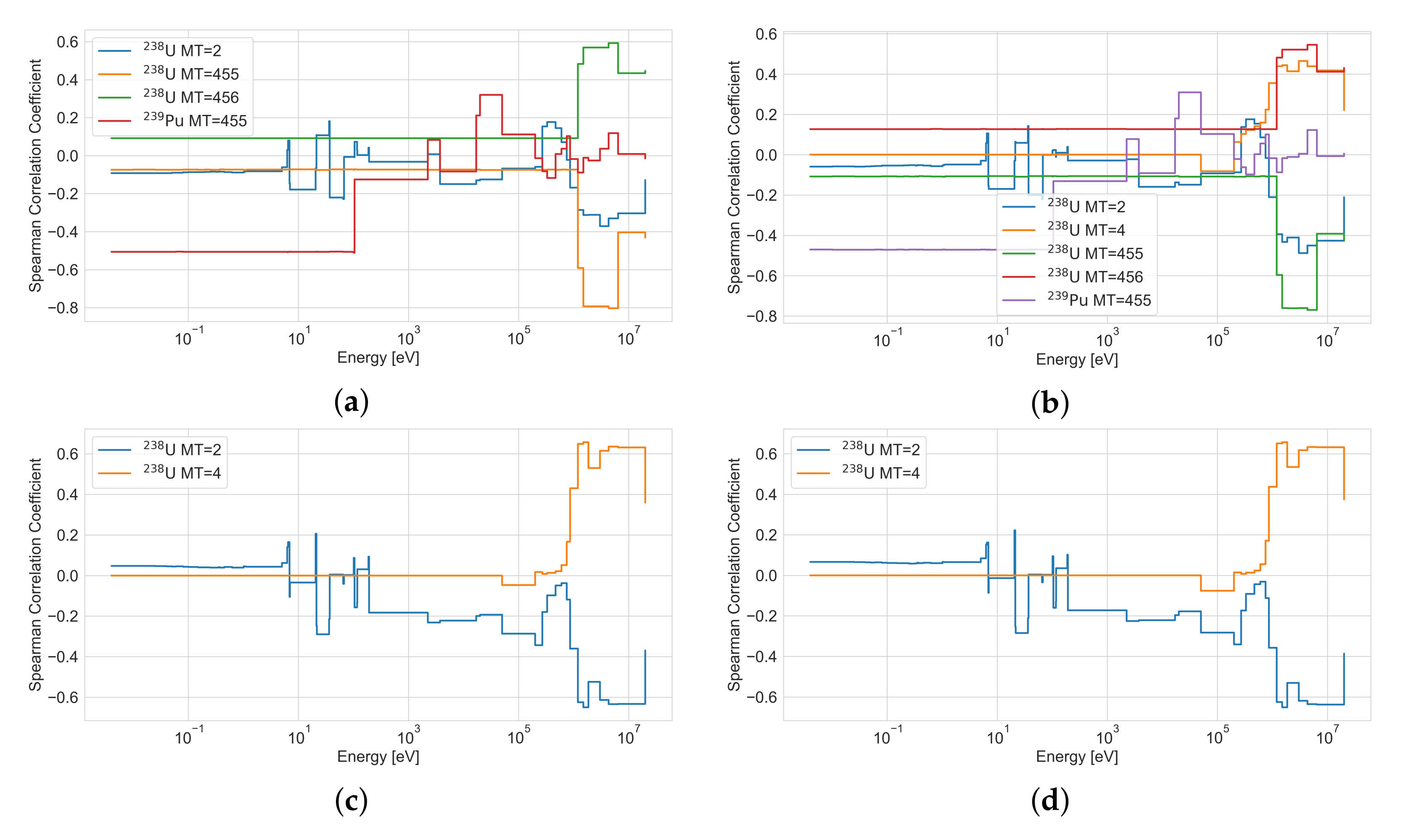
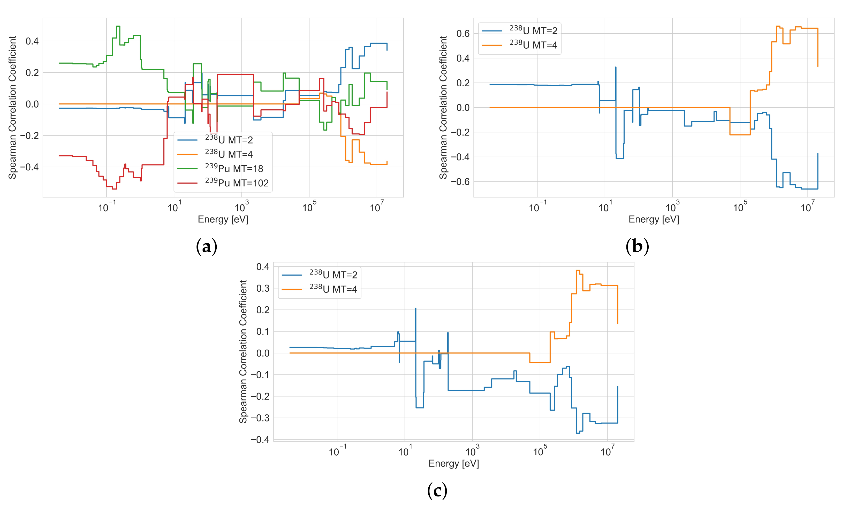
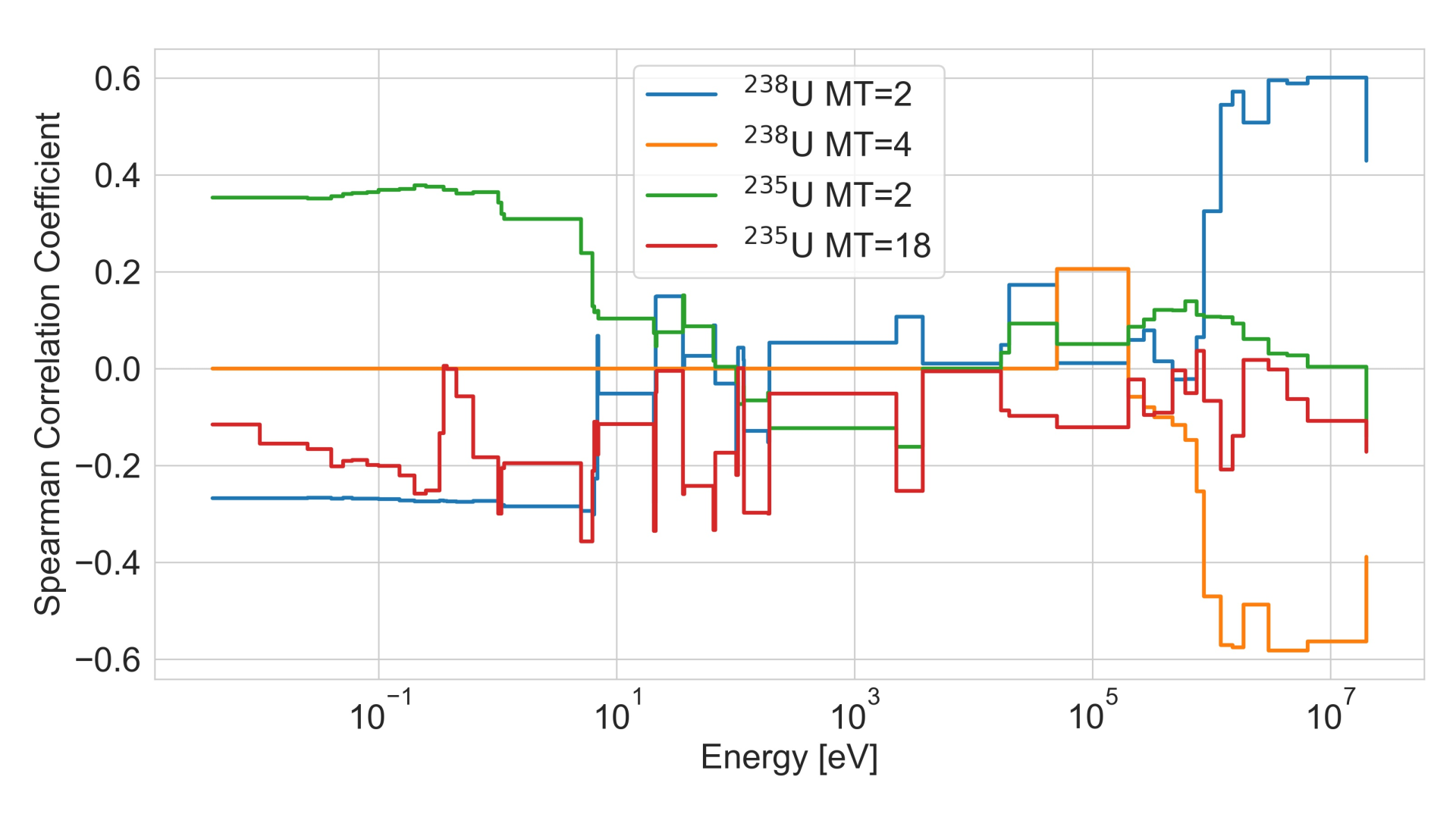
- At BOC steady state, the 235U at low energies (<1 keV) and the 238U inelastic and elastic scattering at high energies (>1 MeV, which corresponds to the 238U inelastic scattering threshold).
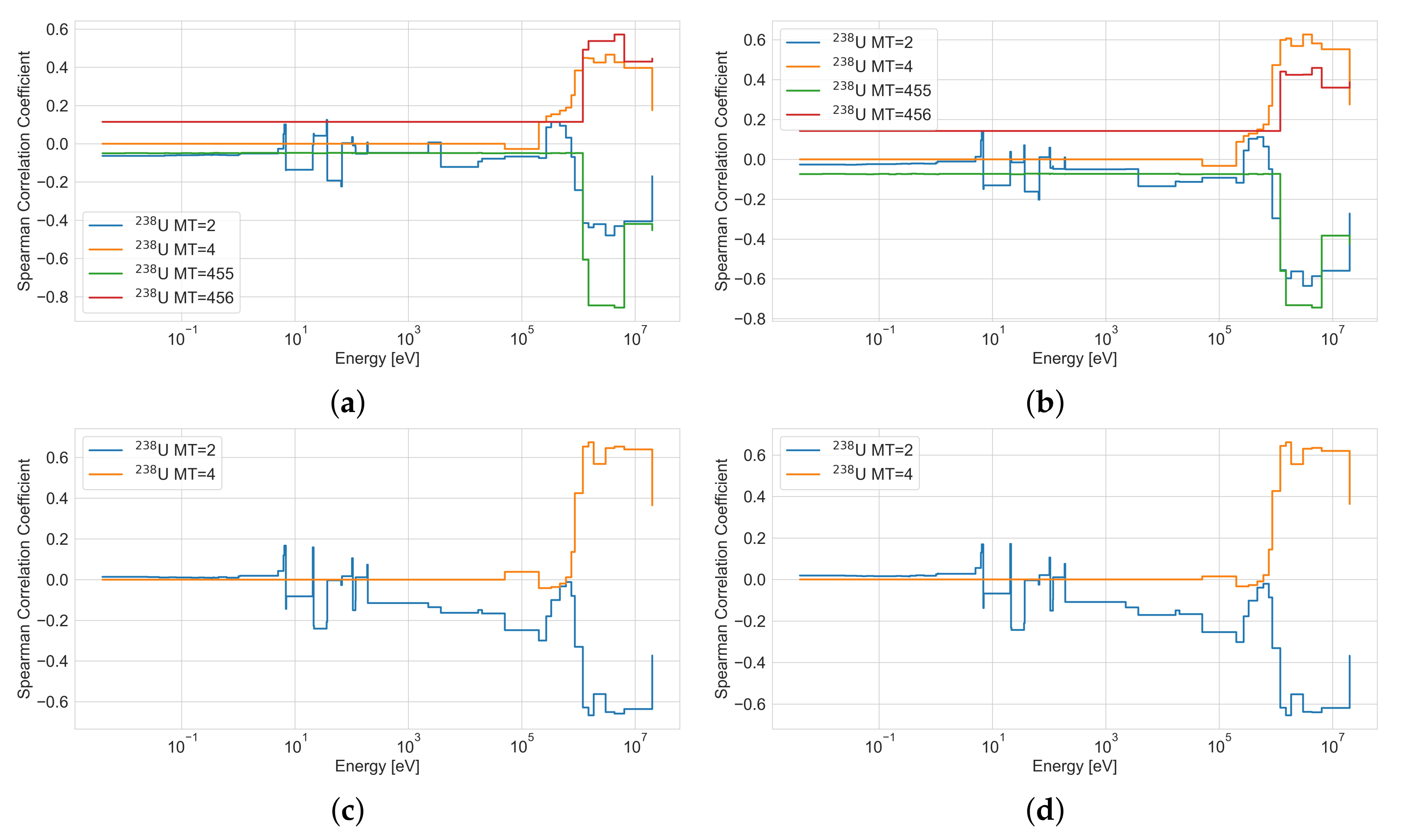
- At BOC REA, the 238U inelastic and elastic scattering at high energies as well as the 238U and at high energies.
- At EOC steady state, the 238U inelastic and elastic scattering at high energies as well as 239Pu fission and capture cross-section at low energies (<10 eV).
- At EOC REA, the 238U inelastic and elastic scattering at high energies, the 238U and , and 239Pu at low energies (<100 eV).
Author Contributions
Funding
Institutional Review Board Statement
Informed Consent Statement
Data Availability Statement
Conflicts of Interest
Abbreviations
| BEPU | Best Estimate Plus Uncertainty |
| BWR | Boiling Water Reactor |
| BOC | Beginning of Cycle |
| CASL | Consortium for Advanced Simulation of Light water reactors |
| DOE | Department of Energy |
| E.C. | European Commission |
| EFPD | Effective Full Power Days |
| EOC | End of Cycle |
| HFP | Hot Full Power |
| HPC | High Performance Computing |
| HZP | Hot Zero Power |
| LWR | Light Water Reactor |
| MPI | Message Passing Interface |
| NEA | Nuclear Energy Angency |
| NCSU | North Carolina State University |
| OECD | Organisation for Economic Co-operation and Development |
| PWR | Pressurized Water Reactor |
| REA | Rod Ejection Accident |
| SCRAM | Safety Control Rod Axe Man |
| TMI | Three Mile Island |
| U.S. | United States |
| VVER | Water Water Energetic Reactor |
References
- Rohatgi, U.S.; Kaizer, J.S. Historical perspectives of BEPU research in US. Nucl. Eng. Des. 2020, 358, 110430. [Google Scholar] [CrossRef]
- Kochunas, B.; Collins, B.; Stimpson, S.; Salko, R.; Jabaay, D.; Graham, A.; Liu, Y.; Seog Kim, K.; Wieselquist, W.; Godfrey, A.; et al. VERA Core Simulator Methodology for Pressurized Water Reactor Cycle Depletion. Nucl. Sci. Eng. 2017, 185, 217–231. [Google Scholar] [CrossRef]
- Lefebvre, R.A.; Langley, B.R.; Miller, P.; Delchini, M.; Baird, M.L.; Lefebvre, J.P. NEAMS Workbench Status and Capabilities; Technical Report ORNL/TM-2019/1314; Oak Ridge National Laboratory, Reactor Nuclear Systems Division: Oak Ridge, TN, USA, 2019. [Google Scholar]
- Permann, C.J.; Gaston, D.R.; Andrš, D.; Carlsen, R.W.; Kong, F.; Lindsay, A.D.; Miller, J.M.; Peterson, J.W.; Slaughter, A.E.; Stogner, R.H.; et al. MOOSE: Enabling massively parallel multiphysics simulation. SoftwareX 2020, 11, 100430. [Google Scholar] [CrossRef]
- Targa, A. Development of Multi-Physics and Multi-Scale Best Effort Modelling of Pressurized Water Reactor under Accidental Situations. Ph.D. Thesis, Université Paris Saclay (COmUE), Saclay, France, 2017. [Google Scholar]
- Fiorina, C.; Clifford, I.; Aufiero, M.; Mikityuk, K. GeN-Foam: A novel OpenFOAM® based multi-physics solver for 2D/3D transient analysis of nuclear reactors. Nucl. Eng. Des. 2015, 294, 24–37. [Google Scholar] [CrossRef]
- Valtavirta, V.; Hovi, V.; Loukusa, H.; Rintala, A.; Sahlberg, V.; Tuominen, R.; Leppänen, J. Kraken: An upcoming Finnish reactor analysis framework. In Proceedings of the International Conference on Mathematics and Computational Methods Applied to Nuclear Science and Engineering (M&C 2019), 25–29 August 2019; American Nuclear Society (ANS): Portland, OR, USA, 2019; pp. 786–795. [Google Scholar]
- Cherezov, A.; Park, J.; Kim, H.; Choe, J.; Lee, D. A Multi-Physics Adaptive Time Step Coupling Algorithm for Light-Water Reactor Core Transient and Accident Simulation. Energies 2020, 13, 6374. [Google Scholar] [CrossRef]
- Hou, J.; Avramova, M.; Ivanov, K. Best-Estimate Plus Uncertainty Framework for Multiscale, Multiphysics Light Water Reactor Core Analysis. Sci. Technol. Nucl. Install. 2020, 2020, 7526864. [Google Scholar] [CrossRef]
- Salko, R., Jr.; Avramova, M.; Wysocki, A.; Toptan, A.; Hu, J.; Porter, N.; Blyth, T.S.; Dances, C.A.; Gomez, A.; Jernigan, C.; et al. CTF 4.0 Theory Manual; CASL, Oak Ridge National Lab: Oak Ridge, TN, USA, 2019. [Google Scholar] [CrossRef]
- Downar, T.; Barber, D.; Matthew Miller, R.; Lee, C.; Kozlowski, T.; Lee, D.; Xu, Y.; Gan, J.; Joo, H.; Cho, J.; et al. PARCS: Purdue advanced reactor core simulator. In Proceedings of the PHYSOR 2002—International Conference on the New Frontiers of Nuclear Technology, 7–10 October, Seoul, Republic of Korea; American Nuclear Society: La Grange Park, IL, USA, 2002. [Google Scholar]
- Wang, J.; Wang, Q.; Ding, M. Review on neutronic/thermal-hydraulic coupling simulation methods for nuclear reactor analysis. Ann. Nucl. Energy 2020, 137, 107165. [Google Scholar] [CrossRef]
- Ivanov, K.; Avramova, M. Challenges in coupled thermal–hydraulics and neutronics simulations for LWR safety analysis. Ann. Nucl. Energy 2007, 34, 501–513. [Google Scholar] [CrossRef]
- Ragusa, J.C.; Mahadevan, V.S. Consistent and accurate schemes for coupled neutronics thermal-hydraulics reactor analysis. Nucl. Eng. Des. 2009, 239, 566–579. [Google Scholar] [CrossRef]
- Senecal, J.P.; Ji, W. Development of an efficient tightly coupled method for multiphysics reactor transient analysis. Prog. Nucl. Energy 2018, 103, 33–44. [Google Scholar] [CrossRef]
- Zhang, H.; Guo, J.; Lu, J.; Niu, J.; Li, F. A comparison of coupling algorithms for N/TH transient problems in HTR. In Proceedings of the International Conference on Mathematics and Computational Methods Applied to Nuclear Science and Engineering (M&C 2017), Jeju, Korea, 16–20 April 2017. [Google Scholar]
- Zhang, H.; Guo, J.; Lu, J.; Li, F.; Xu, Y.; Downar, T.J. An Assessment of Coupling Algorithms in HTR Simulator TINTE. Nucl. Sci. Eng. 2018, 190, 287–309. [Google Scholar] [CrossRef]
- Hamilton, S.; Berrill, M.; Clarno, K.; Pawlowski, R.; Toth, A.; Kelley, C.; Evans, T.; Philip, B. An assessment of coupling algorithms for nuclear reactor core physics simulations. J. Comput. Phys. 2016, 311, 241–257. [Google Scholar] [CrossRef] [Green Version]
- Ellis, M.; Watson, J.; Ivanov, K. Progress in the development of an implicit steady state solution in the coupled code TRACE/PARCS. Prog. Nucl. Energy 2013, 66, 1–12. [Google Scholar] [CrossRef]
- Ivanov, K.; Avramova, M.; Kamerow, S.; Kodeli, I.; Sartori, E.; Ivanov, E.; Cabellos, O. Benchmarks for Uncertainty Analysis in Modelling (UAM) for the Design, Operation and Safety Analysis of LWRs, Volume I: Specification and Support Data for Neutronics Cases (Phase I); OECD Nuclear Energy Agency: Paris, France, 2013. [Google Scholar]
- Delipei, G.K. Development of an Uncertainty Quantification methodology for Multi-Physics Best Estimate Analysis and Application to the Rod Ejection Accident in a Pressurized Water Reactor. Ph.D. Thesis, Université Paris Saclay (COmUE), Saclay, France, 2019. [Google Scholar]
- Kaiyue, Z. Uncertainty Analysis Framework for the Multi-Physics Light Water Reactor Simulation. Ph.D. Thesis, North Carolina State University, Raleigh, NC, USA, 2020. [Google Scholar]
- U.S. NRC. TRACE V5.0 Theory Manual, Field Equations, Solution Methods, and Physical Models; Technical Report; U.S. NRC: Washington, DC, USA, 2007. [Google Scholar]
- Hou, J.; Avramova, M.; Ivanov, K.; Royer, E.; Jessee, M.; Zhang, J.; Wieselquist, W.; Pasichnyk, I.; Zwermann, W.; Velkov, K.; et al. Benchmarks for Uncertainty Analysis in Modelling (UAM) for the Design, Operation and Safety Analysis of LWRs, Volume III: Specification and Support Data for the System Cases (Phase III); OECD Nuclear Energy Agency: Paris, France, 2019. [Google Scholar]
- Jessee, M.A.; Wieselquist, W.A.; Evans, T.M.; Hamilton, S.P.; Jarrell, J.J.; Kim, K.S.; Lefebvre, J.P.; Lefebvre, R.A.; Mertyurek, U.; Thompson, A.B.; et al. POLARIS: A New Two-Dimensional Lattice Physics Analysis Capability for the SCALE Code System; Oak Ridge National Laboratory (ORNL): Oak Ridge, TN, USA, 2014. [Google Scholar]
- Rearden, B.T.; Jessee, M.A. SCALE Code System, Version 6.2.3; Technical Report ORNL/TM-2005/39; Oak Ridge National Laboratory, Reactor and Nuclear Systems Division: Oak Ridge, TN, USA, 2018. [Google Scholar]
- Chadwick, M.B.; Obložinský, P.; Dunn, M.; Danon, Y.; Kahler, A.; Smith, D.; Pritychenko, B.; Arbanas, G.; Arcilla, R.; Brewer, R.; et al. ENDF/B-VII.1 Nuclear Data for Science and Technology: Cross Sections, Covariances, Fission Product Yields and Decay Data. Nucl. Data Sheets 2011, 112, 2887–2996. [Google Scholar] [CrossRef]
- Ward, A.; Xu, Y.; Downar, T. GenPMAXS-v6.1.3—Code for Generating the PARCS Cross Section Interface File PMAXS; Technical Report; University of Michigan: Ann Arbor, MI, USA, 2015. [Google Scholar]
- U.S. DOE. CASL Phase II Summary Report; Technical Report CASL-U-2020-1974-000; ORNL/SPR-2020/1759; CASL; 2020. Available online: https://casl.gov/wp-content/uploads/2020/11/CASL_FINAL_REPORT_09.30.2020-002.pdf (accessed on 13 July 2022).
- European Commission. NURESAFE Project Final Report. Technical Report GA N° 323263; E.C.. 2016. Available online: https://cordis.europa.eu/docs/results/323/323263/final1-nuresafe-final-report-publishable-summary-june-29-2016.pdf (accessed on 13 July 2022).
- Dalbey, K.; Eldred, M.S.; Geraci, G.; Jakeman, J.D.; Maupin, K.A.; Monschke, J.A.; Seidl, D.T.; Swiler, L.P.; Tran, A.; Menhorn, F.; et al. Dakota A Multilevel Parallel Object-Oriented Framework for Design Optimization Parameter Estimation Uncertainty Quantification and Sensitivity Analysis: Version 6.12 Theory Manual; Sandia National Laboratories: Albuquerque, NM, USA, 2020. [Google Scholar] [CrossRef]
- Abarca, A.; Avramova, M.; Kostadin, I. Development of a General MPI Coupling Interface for Multi-Physics Analysis; ANS International Conference on Mathematics and Computational Methods Applied to Nuclear Science and Engineering: Lucca, Italy, 2021. [Google Scholar]
- Rowlands, G. Resonance absorption and non-uniform temperature distributions. J. Nucl. Energy. Parts A/B. React. Sci. Technol. 1962, 16, 235–236. [Google Scholar] [CrossRef]
- Bernard, D.; Calame, A.; Palau, J.M. LWR-UOx doppler reactivity coefficient best estimate plus (nuclear and atomic sources of) uncertainties. In Proceedings of the M&C—2017 International Conference on Mathematics & Computational Methods Applied to Nuclear Science & Engineering, Jeju, Korea, 16–20 April 2017. [Google Scholar]
- Lassmann, K.; O’Carroll, C.; van de Laar, J.; Walker, C. The radial distribution of plutonium in high burnup UO2 fuels. J. Nucl. Mater. 1994, 208, 223–231. [Google Scholar] [CrossRef]
- Iooss, B.; Marrel, A. An efficient methodology for the analysis and modeling of computer experiments with large number of inputs. In Proceedings of the UNCECOMP 2017 2nd ECCOMAS Thematic Conference on Uncertainty Quantification in Computational Sciences and Engineering, Rhodes Island, Greece, 15–17 June 2017; pp. 187–197. [Google Scholar]
- Hou, J.; Blyth, T.; Porter, N.; Avramova, M.; Ivanov, K.; Royer, E.; Sartori, E.; Cabellos, O.; Feroukhi, H.; Ivanov, E. Benchmarks for Uncertainty Analysis in Modelling (UAM) for the Design, Operation and Safety Analysis of LWRs, Volume II: Specification and Support Data for the Core Cases (Phase II); OECD Nuclear Energy Agency: Paris, France, 2019. [Google Scholar]
- Zeng, K.; Hou, J.; Ivanov, K.; Jessee, M.A. Uncertainty Quantification and Propagation of Multiphysics Simulation of the Pressurized Water Reactor Core. Nucl. Technol. 2019, 205, 1618–1637. [Google Scholar] [CrossRef]
- Porter, N.W. Wilks’ formula applied to computational tools: A practical discussion and verification. Ann. Nucl. Energy 2019, 133, 129–137. [Google Scholar] [CrossRef]
- Delipei, G.K.; Hou, J.; Avramova, M.; Rouxelin, P.; Ivanov, K. Summary of comparative analysis and conclusions from OECD/NEA LWR-UAM benchmark Phase I. Nucl. Eng. Des. 2021, 384, 111474. [Google Scholar] [CrossRef]
- Roy, C.J.; Oberkampf, W.L. A comprehensive framework for verification, validation, and uncertainty quantification in scientific computing. Comput. Methods Appl. Mech. Eng. 2011, 200, 2131–2144. [Google Scholar] [CrossRef]
- Dokhane, A.; Vasiliev, A.; Hursin, M.; Rochman, D.; Ferroukhi, H. A critical study on best methodology to perform UQ for RIA transients and application to SPERT-III experiments. Nucl. Eng. Technol. 2021, 54, 1804–1812. [Google Scholar] [CrossRef]
- Delipei, G.K.; Garnier, J.; Le Pallec, J.; Normand, B. Multi-Physics Uncertainties Propagation in a PWR Rod Ejection Accident Modeling—Analysis Methodology and First Results; ANS Best Estimate Plus Uncertainty International Conference (BEPU 2018): Lucca, Italy, 2018. [Google Scholar]


| MT | Reaction |
|---|---|
| 2 | Elastic scattering |
| 4 | Inelastic scattering |
| 18 | Fission |
| 102 | Radiative capture |
| 455 | : delayed neutrons released per fission |
| 456 | : prompt neutrons released per fission |
| 1018 | Fission spectrum |
| Input | Variable | Probability Density Function |
|---|---|---|
| Fuel Thermal Conductivity | N (1.0, 0.00774) | |
| Cladding Thermal Conductivity | N (1.0, 0.00559) | |
| Fuel Specific Heat Capacity | N (1.0, 0.015) | |
| Cladding Specific Heat Capacity | N (1.0, 0.015) | |
| Gap Conductance | U (0.75, 1.25) | |
| Outlet Pressure | N (1.0, 0.005) | |
| Inlet Mass Flux | N (1.0, 0.001) | |
| Inlet Coolant Temperature | N (1.0, 0.00267) |
| Input | Variable | Units | Probability Density Function |
|---|---|---|---|
| 235U enrichment | w/o% | N (4.95, 0.000746) | |
| density | N (10.283, 0.0566) | ||
| density | N (10.14, 0.0566) | ||
| Fuel outer radius | cm | N (0.46955, 0.000433) | |
| Cladding inner radius | cm | N (0.4791, 0.0008) | |
| Cladding outer radius | cm | N (0.5464, 0.00083) | |
| Instrumentation tube outer radius | cm | N (0.6261, 0.00083) | |
| Control rod outer radius | cm | N (0.6731, 0.00083) | |
| Guide tube outer radius | cm | N (0.6731, 0.00083) |
| Parameter | Variable | Units | Min | Max |
|---|---|---|---|---|
| Fuel temperature | 560 | 1600 | ||
| Moderator density | 0.60811 | 0.76971 | ||
| Boron concentration | 0 | 1800 | ||
| Control rod insertion | - | - | 0 | 1 |
| Output Quantity | Description | Variable |
|---|---|---|
| Scalar | Maximum linear power in the 3D core | |
| Maximum fuel centerline temperature in the 3D core | ||
| Minimum coolant density in the 3D core | ||
| Effective multiplication factor | ||
| Functional 1D | Radially averaged axial linear power | |
| Radially averaged axial fuel centerline temperature | ||
| Radially averaged axial coolant temperature | ||
| Radially averaged axial coolant density | ||
| Functional 2D | Axially averaged radial linear power | |
| Axially averaged radial fuel centerline temperature |
| Output Quantity | Description | Variable |
|---|---|---|
| Scalar | Maximum linear power during the transient | |
| Maximum fuel centerline temperature during the transient | ||
| Maximum fuel enthalpy during the transient | ||
| Inserted reactivity | ||
| Functional 1D | Maximum linear power over time | |
| Maximum fuel centerline temperature over time | ||
| Maximum fuel enthalpy over time | ||
| Functional 2D | Axially averaged radial linear power, end of the transient | |
| Axially averaged radial fuel centerline temperature, end of the transient |
| Output Quantity | Description | Variable |
|---|---|---|
| Scalar | Average burnup at EOC | |
| Maximum burnup at EOC | ||
| 1D Functional | Maximum linear power over depletion | |
| Maximum fuel centerline temperature over depletion | ||
| Maximum burnup over depletion | ||
| Radially averaged axial linear power at BOC | ||
| Radially averaged axial linear power at EOC | ||
| Radially averaged axial burnup at EOC | ||
| 2D Functional | Axially averaged radial burnup at EOC |
Publisher’s Note: MDPI stays neutral with regard to jurisdictional claims in published maps and institutional affiliations. |
© 2022 by the authors. Licensee MDPI, Basel, Switzerland. This article is an open access article distributed under the terms and conditions of the Creative Commons Attribution (CC BY) license (https://creativecommons.org/licenses/by/4.0/).
Share and Cite
Delipei, G.K.; Rouxelin, P.; Abarca, A.; Hou, J.; Avramova, M.; Ivanov, K. CTF-PARCS Core Multi-Physics Computational Framework for Efficient LWR Steady-State, Depletion and Transient Uncertainty Quantification. Energies 2022, 15, 5226. https://doi.org/10.3390/en15145226
Delipei GK, Rouxelin P, Abarca A, Hou J, Avramova M, Ivanov K. CTF-PARCS Core Multi-Physics Computational Framework for Efficient LWR Steady-State, Depletion and Transient Uncertainty Quantification. Energies. 2022; 15(14):5226. https://doi.org/10.3390/en15145226
Chicago/Turabian StyleDelipei, Gregory K., Pascal Rouxelin, Agustin Abarca, Jason Hou, Maria Avramova, and Kostadin Ivanov. 2022. "CTF-PARCS Core Multi-Physics Computational Framework for Efficient LWR Steady-State, Depletion and Transient Uncertainty Quantification" Energies 15, no. 14: 5226. https://doi.org/10.3390/en15145226
APA StyleDelipei, G. K., Rouxelin, P., Abarca, A., Hou, J., Avramova, M., & Ivanov, K. (2022). CTF-PARCS Core Multi-Physics Computational Framework for Efficient LWR Steady-State, Depletion and Transient Uncertainty Quantification. Energies, 15(14), 5226. https://doi.org/10.3390/en15145226