1. Introduction
The pursuit of the miniaturisation of electric energy conversion devices requires an increase in switching frequency [
1,
2]. The factor limiting this increase in frequency are dynamic properties of semiconductor and magnetic elements (including the inductor) contained in the mentioned devices [
1,
3,
4,
5]. Additionally, the increasing application requirements in the field of designing devices characterised by high watt-hour efficiency and their failure-free operation force the manufacturers of electronic components and systems to design and produce systems characterised by very high reliability [
6,
7].
In order to obtain a long lifetime of electronic components, an effective cooling system is indispensable. Some forced cooling systems are described in [
8,
9], but for magnetic devices typically free cooling systems are used.
Computer software supporting the work of designers is used to analyse the properties of electronic components and systems. One of the popular kinds of software of this type is SPICE [
10]. This software can use averaged models of switch-mode power supplies [
11,
12,
13]. The mentioned models allow the values of currents and voltages at steady state to be computed using fast DC analysis, instead of time-consuming transient analysis. On the other hand, such models ignore, for example, the non-linearity and inertia of semiconductor devices and the non-linear dependence L(i) of magnetic components [
11].
To take into account the influence of thermal phenomena (such as self-heating and mutual thermal couplings between components of an electronic component) occurring in electronic elements on their electrical characteristics, electrothermal models are used [
13,
14,
15,
16].
In the literature, electrothermal models of semiconductor and magnetic elements are described [
17,
18,
19,
20,
21]. However, in the case of magnetic elements, the mentioned models are limited to classic inductors (single-winding inductors) or transformers [
11,
22], yet there are no such models for coupled inductors.
For example, in [
23], an electrothermal model of an inductor with a ferromagnetic core based on the isothermal Jiles–Atherton model is proposed. Although this model takes into account the self-heating phenomenon, the hysteresis of the magnetisation curve, the energy losses in the core, and the windings, it is a model of an inductor with only one winding. This means that it does not take into account thermal mutual couplings in the case of a larger number of windings.
On the other hand, in [
24], an electrothermal model of the inductor is proposed that takes into account the self-heating phenomenon, but only in the core. This model ignores thermal phenomena occurring in the windings, the skin effect, and the mutual thermal couplings between the windings.
The papers [
11,
25,
26] present inductor models dedicated to operating in electrical conversion systems. The model proposed in [
25] is based on matching the dependence of inductance on the direct current of the inductor using a polynomial function. However, the presented model does not take into account thermal phenomena in the considered element. The model was verified in a buck converter system.
In turn, in [
11,
26] a model of a classic inductor with one winding is proposed. This model takes into account thermal phenomena occurring in the inductor and thermal couplings between its components. The mentioned model also takes into account the capacity of the winding, the skin effect, and the frequency of the control signal when the inductor is operating in the electrical energy conversion system. Unfortunately, this model does not take into account the case of several windings wound on one core, the magnetic coupling between individual windings, or the thermal coupling between them.
In the model previously elaborated by the authors [
27], a model of a coupled inductor dedicated to operating in electrical energy systems is proposed. However, the proposed model does not take into account the skin effect or thermal phenomena occurring in this element. Additionally, the cited paper includes an extensive description of current solutions in the field of application and modelling of the coupled inductors. In the mentioned paper, it is also noted that the T-type transformer model is generally adopted as the main model for formulating a coupled inductor model. This model is the basic model of the transformer, with the structure described in [
28] containing three coils with a common node.
However, in [
29], it is noticed that the T-type transformer model is asymmetric in relation to the symmetrical structure of the transformer and insufficient for the analysis of systems such as, e.g., a multi-phase DC–DC buck converter, because it has magnetising inductance only in one of the windings [
30].
The analysis shows that there are no electrothermal models of coupled inductors dedicated to operating in electrical conversion systems.
This paper presents a new electrothermal model of the coupled inductors dedicated to the analysis of electrical energy conversion systems. The form of the model is described. Some results of measurements and computations confirming the usefulness of this model are also presented.
Section 2 presents the form of a new electrothermal model of coupled inductors.
Section 3 describes the method of estimating the parameters of the formulated model.
Section 4 discusses the element selected for the investigations and the measuring setup used. The obtained results of the measurements and the calculations are included in
Section 5.
2. Model Form
In order to formulate an electronic component model, it is necessary to define the appropriate equations describing phenomena occurring in the considered element. The parameters appearing in the formulated dependences are determined from the performed measurements or from the catalogue data [
27].
This section proposes a new electrothermal model of coupled inductors dedicated to the analysis of electrical energy conversion systems. This model is based on the model presented in paper [
27] and represents a coupled inductor containing any number of windings
n. The new model additionally takes into account the skin effect, self-heating phenomena, and mutual thermal coupling between inductor components. All the mentioned phenomena were omitted in the presented model in paper [
27]. Due to the simplification of the description and the improvement of its comprehensibility, the considerations are limited to the case where the coupled inductor contains three windings. The considerations were carried out for an inductor with a nanocrystalline core. The proposed model is in the form of a subcircuit for SPICE. The network representation of this model is shown in
Figure 1.
The developed model consists of three blocks: the main circuit, the auxiliary circuit, and the thermal model. The structure of the proposed model is shown in
Figure 2. This model takes into account the influence of frequency, skin effect, direct current, temperature, and thermal phenomena on the characteristics of the coupled inductors.
The main circuit describes the properties of individual windings of the modelled inductors connected between terminals Ai and Bi (i = 1 … n). The model of each winding consists of six series of connected elements: a voltage source with zero efficiencies VLSi; a linear inductor with inductance Li; controlled voltage sources ELSi, EMi, and ERSi; and a resistor RSi. The capacitor Ci, connected in parallel to the terminals Ai and Bi, represents parasitic capacitance of the winding.
The controlled voltage source E
LSi represents the inductance of the i-th inductor winding, and its efficiency is described by the following formula [
11]:
where z
i is the number of winding turns, S
Fe is the cross-section area of the core, B
sat is the saturation of the magnetic flux density, A is the field parameter, H is the magnetic force, l
Fe is the magnetic path length, l
p is the air gap length, a
i is the scaling factor, and V
Li is the voltage on a linear inductor L
i.
The controlled voltage source E
Mi represents the mutual inductance between the i-th winding and the other windings, expressed by the following formula [
27]:
where k
j is the magnetic coupling coefficient, V
ELSj is the voltage at the source E
LSj, and n is the number of inductor windings.
The controlled voltage source E
SRi represents a voltage drop in the series resistance of the inductor as a result of the skin effect and self-heating. Its efficiency is described by the following formula [
11]:
where V
RSi denotes the voltage on the resistor R
Si; d
d is the diameter of the winding wire; l
d is the length of the winding; α
p is the temperature coefficient of copper resistivity; T
Wi, T
a, and T
0 are the winding temperature, ambient temperature, and reference temperature, respectively; µ
0 is the magnetic permeability of the vacuum, ρ is the copper resistivity, and i
Li is the current flowing through the i-th inductor winding.
In turn, the resistance value of the resistor R
Si corresponds to the series resistance of a single winding for the direct current and temperature T
0. The value of this resistance is calculated from the classical formula
The auxiliary circuit block consists of two controlled voltage sources, EB and EH, used to determine the magnetic flux density of the core B and the magnetic force, respectively. The efficiencies of these sources are described by the dependences [
31,
32]
where i
i is the current of the i-th winding.
Due to the very narrow hysteresis loops of the considered inductor core in the model, the core losses are neglected.
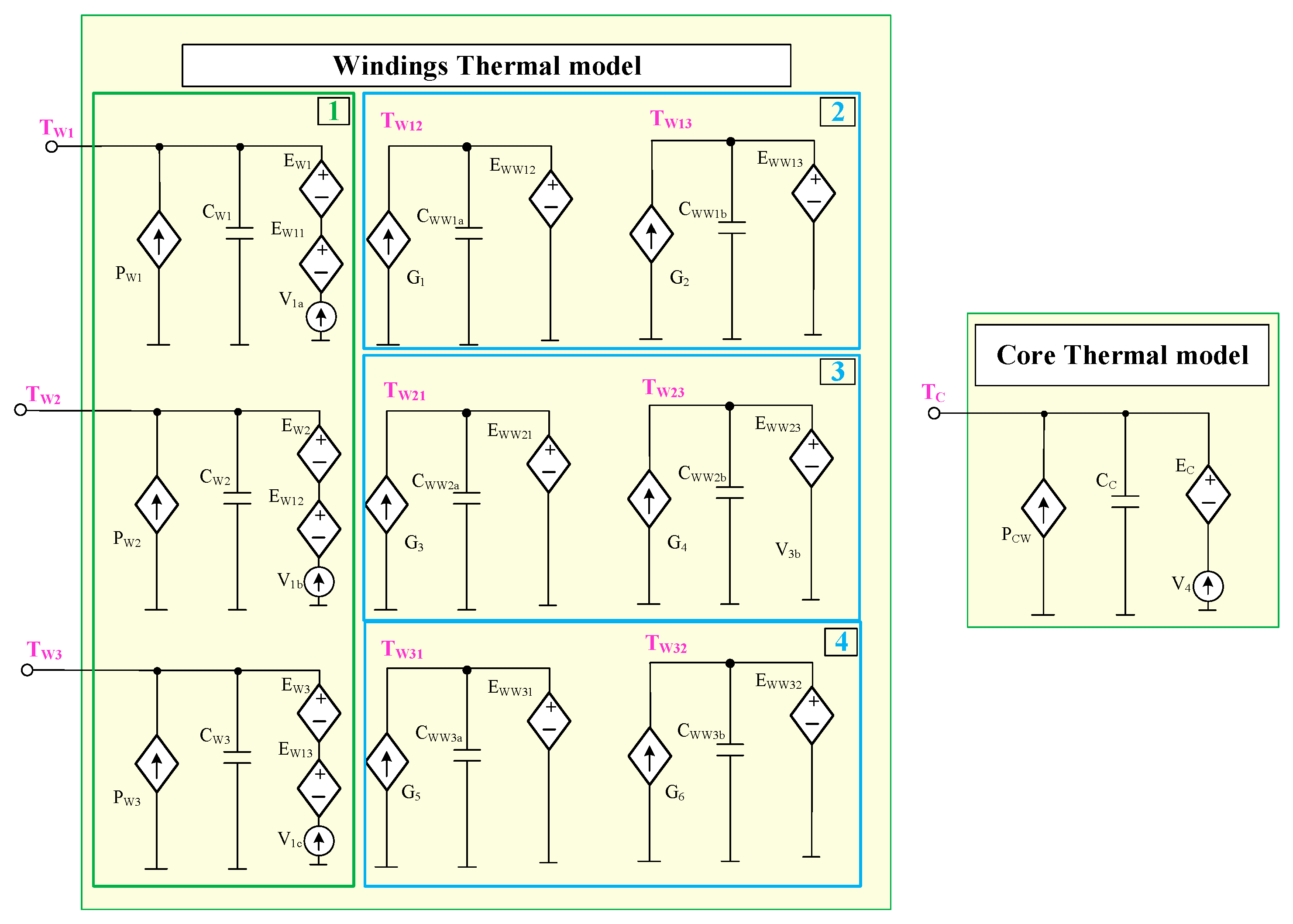
In turn, the thermal model (
Figure 2) is used to determine the temperature of each winding T
W1, T
W2, and T
W3, and the temperature of the core T
C of the coupled inductor. This model takes into account the phenomenon of self-heating in each winding and thermal coupling between each pair of windings and between each winding and the core.
This model consists of 10 subcircuits, nine of which are included in the thermal model of the winding and one in the thermal model of the core. For better readability of the model description, the thermal model of the winding was divided into four blocks. Block 1, contained in the thermal model of the winding, includes three subcircuits for determining the temperature of the first winding TW1, the second winding TW2, and the third winding TW3, taking into account the self-heating in each of them and mutual thermal couplings. The subcircuits included in blocks 2, 3, and 4 are used to determine a temperature rise resulting from the mutual thermal coupling between the windings. In block 2, a temperature rise in the first winding caused by heat generation in the second (TW12) winding and a temperature rise in the first winding caused by heat generation in the third (TW13) winding are determined. The subcircuits in block 3 make it possible to determine a temperature rise in the second winding caused by heat generation in the first winding (TW21) and in the third winding (TW23). On the other hand, block 3 is used to determine temperature increases in the third winding caused by heat generation in the first (TW31) and second (TW32) windings. The proposed thermal winding model includes nine controlled current sources. Three of them are included in block 1, where they represent the power dissipated in each winding PW1, PW2, and PW3. The controlled current sources G1, G2, G3, G4, G5, and G6 included in blocks 2, 3, and 4 represent the power dissipated in the first winding PW1 (G3, G5), the second winding PW2 (G1, G6), and the third winding PW3 (G2, G4). However, the thermal model of the core contains one controlled PCW current source, the efficiency of which corresponds to the sum of the power dissipated in each winding (PW1 + PW2 + PW3).
The controlled voltage sources EW1, EW2, and EW3 included in the thermal model of the windings model the nonlinear thermal resistance of individual windings.
As per the literature [
16,
19,
33,
34] and the measurements made, thermal resistance is a non-linear function of temperature and the number of windings n, in which the power is dissipated.
In the considered case of coupled inductors, the efficiency of these sources is the same and described by the empirical dependence
where P
Wi is the power dissipated in the i-th winding; T
W is the temperature of the winding in which the power is dissipated; w
1 and α are the scaling coefficients, taking into account the number of windings in which the power is dissipated; R
thW0 is the minimum value of thermal resistance of the winding; R
thW1 is the maximum change value of the winding thermal resistance; T
zW determines the slope of R
thW(T
W); and n
U is the number of windings in which the power is simultaneously dissipated.
The controlled voltage source E
C models the nonlinear thermal resistance between the winding and the core R
thCW. The efficiency of this source is described by the empirical dependence
where T
C is the core temperature; w
2 and w
22 are the scaling coefficients, taking into account the influence of the number of windings in which the power is dissipated on mutual thermal resistance between the core and the winding; R
thC0 is the minimum value of mutual thermal resistance between the core and the winding; R
thC1 is the maximum change in the value of this resistance temperature; T
zC determines the slope of R
thC(T
C); and P
CW is the power dissipated in the winding.
In turn, the controlled voltage sources E
W11, E
W12, and E
W13 model a temperature increase in individual windings resulting from thermal couplings between individual windings. The efficiency of these sources is described by the following empirical formula:
where T
W12, T
W13, T
W21, T
W23, T
W31, and T
W32 denote the temperature rises in individual windings caused by thermal couplings, which are determined in blocks 2, 3, and 4.
The controlled voltage sources E
WW12, E
WW13, E
WW21, E
WW23, E
WW31, and E
WW32 model mutual thermal resistance between the windings. The description of the efficiency of these sources for each pair of windings is the same and is described by the following empirical formula:
where T
W2 is the temperature of winding 2, where no power is dissipated; R
thWW0 is the minimum value of mutual thermal resistance between the windings; R
thW1 is the maximum change in the value of mutual thermal resistance between the windings; and i
WWi is the current of the source G
i.
The voltage sources V1a, V1b, V1c, V2a, and V4 model the ambient temperature Ta.
4. Investigated Device and Measurement Setup
In the investigations, a coupled inductor with compensation type DK3H-3352-1011-NK made by Schurter (
Figure 3) was used. It contains a toroidal nanocrystalline core in the housing made of plastic of the UL 94V-0 flammability class. The dimensions of the considered coupled inductor are an external diameter of 38.3 mm, internal diameter of 25.3 mm, and height of 15.2 mm. Three windings made of enamelled copper wire with a diameter of 1.1 mm are wound on the core [
36]. Each winding contains 11 turns.
In order to verify the correctness of the developed model, the influence of temperature and the direct winding current on the parameters of the coupled inductor were investigated.
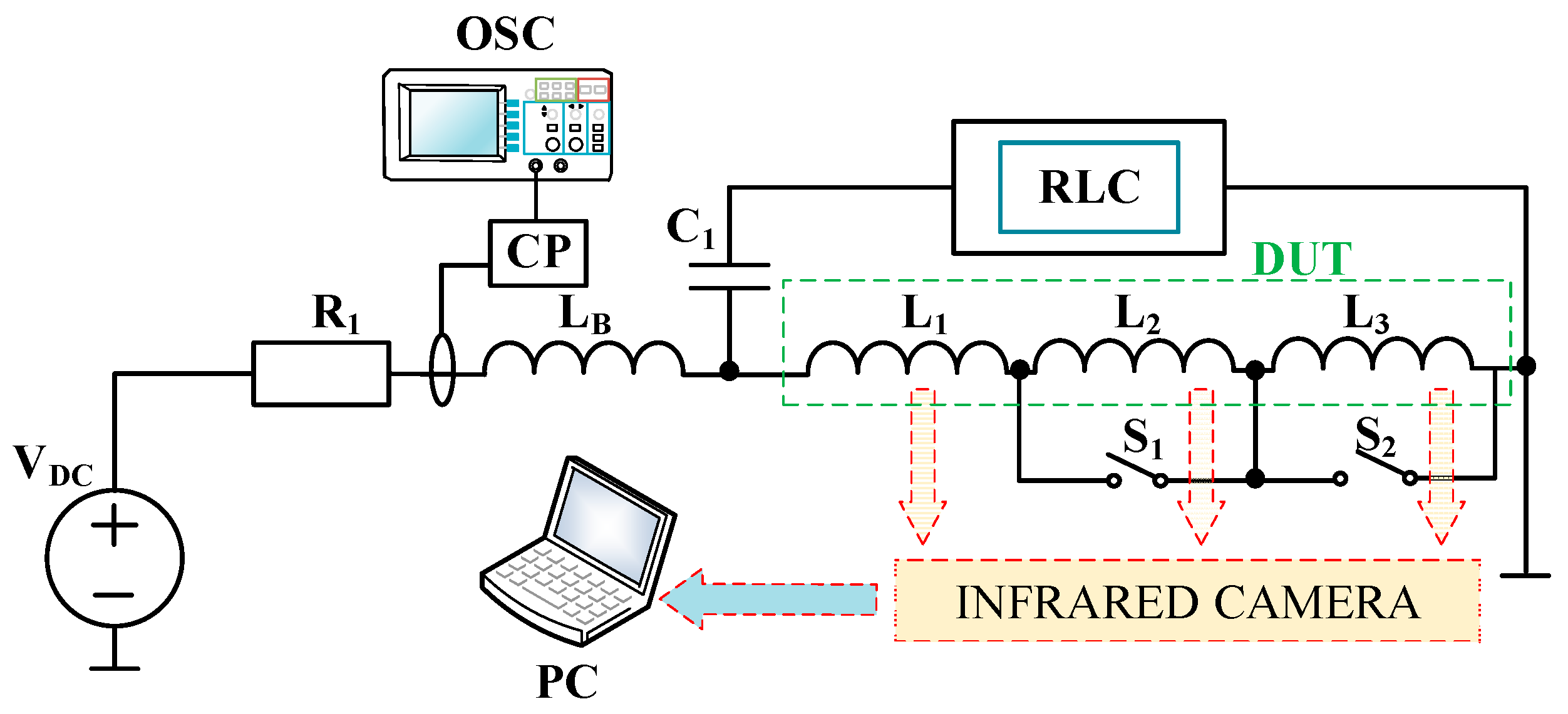
To determine the coupled inductor parameters, the measurement setup shown in
Figure 4 was used.
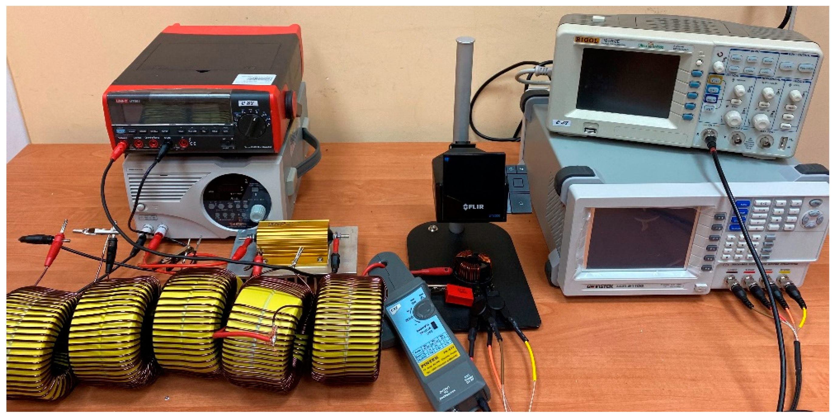
Figure 5 shows a photo of the measurement setup used.
In the setup presented in
Figure 4, the windings of the investigated element were marked with the symbols L
1, L
2, and L
3. Depending on the position of switches S
1 and S
2, the dependence of the inductor inductance on its current was measured when the current flowed through one winding L
1, two windings L
1 and L
2, or three windings L
1, L
2, and L
3. The resistor R
1 of the resistance equal to 1 Ω limited the current of the DC voltage source V
DC. If the value of this current ranged from 0 to 10 A, it was measured with the multimeter UNIT-T 804. In turn, if this current exceeded 10 A it was measured using the oscilloscope (OSC) of the type RIGOL DS 1052E with the current probe (CP) of the type PINTEK PA-677.
The capacitor C
1, with a capacity of 6.7 µF, protected the RLC bridge, making a flow of the direct current through this bridge impossible. In turn, the inductor L
B, with an inductance of 1.45 mH, reduced the value of the alternating current of the voltage source V
DC. The automatic bridge GWINSTEK LCR-8110G [
37] was used to measure the inductance of the investigated element. During the measurements, the LCR bridge worked in the mode of measurement inductance with series equivalent resistance. Additionally, by using the FLIR ETS-320 (INFRARED CAMERA) [
38] infrared camera connected to a computer, the temperature distribution was recorded on all the components of the investigated inductor.
In order to ensure a reliable measurement result, it was necessary to keep the relation of Li >> LB. The LB contained the powdered iron core (type 102 material) with 20 turns of copper wire in enamel with a diameter 2 mm. The geometric dimensions of the inductor were as follows: outer diameter of 10.3 cm, inner diameter of 5.6 cm, and height of 6.5 cm.
Figure 6 shows the measured dependence L
B(I
DC) of the blocking inductor. The measurements were made in the circuit shown in
Figure 4. As a blocking inductor, a series connection of five identical inductors connected in series was used.
As can be seen in
Figure 6, the dependence of inductance L
B of the blocking inductor on the direct current I
DC in the range of 0 to 5 A was almost constant. For I
DC > 5 A the inductance of the inductor decreased to the value of approx. 800 µH at I
DC = 19 A.
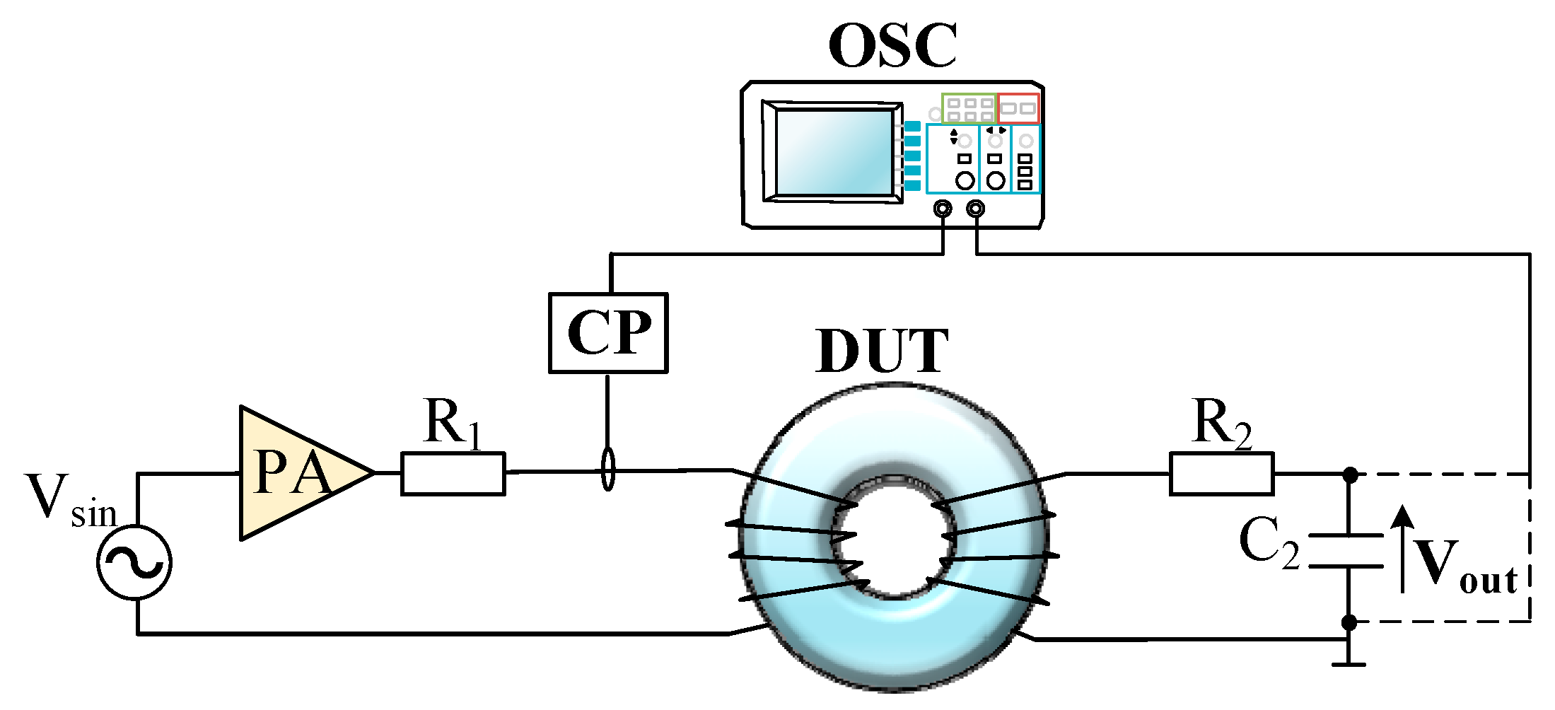
In turn, in order to characterise parameters of the nanocrystalline core of the considered coupled inductor and to determine its saturation of magnetic flux density B
sat, the hysteresis loop was measured using the classic measurement system shown in
Figure 7 [
31,
32].
In the measurement setup presented in
Figure 7, the JV5603P function generator was used as the source of the sinusoidal input signal V
sin [
39]. To amplify the input signal, the AETECHRON 7228 power amplifier (PA) was used [
40]. The resistor R
1 was used to limit the current flowing from the source V
sin, and the resistor R
2 and the capacitor C
2 represented the integrator. By recording with the RIGOL1102D [
41] oscilloscope (OSC), the input current waveforms using the current probe (CP) PINTEK PA / 677 [
42], and the voltage time waveform on the capacitor C
2, the time waveform of the magnetic force from the dependence (6) was determined, and the magnetic flux density was determined from the dependence:
Figure 8 shows the hysteresis loop of the investigated nanocrystalline core obtained with the use of the measurement setup shown in
Figure 7. The measurements were carried out at the input signal frequency f = 2.6 kHz. The resistance values of the resistor R
1 and R
2 were 0.5 Ω and 100 Ω, respectively, whereas the capacitance of the C
2 capacitor was equal to 3.19 µF.
As can be seen, the investigated core was characterised by a low value of the saturation of magnetic flux density Bsat equal to 110 mT and low power losses presented by a very narrow hysteresis loop.
Based on the estimation procedure described in
Section 3, the values of the parameters of the electrothermal model of the investigated inductor were determined and are collected in
Table 1,
Table 2 and
Table 3.
Table 1,
Table 2 and
Table 3 summarise the values of the geometric parameters, the magnetic parameters, and the thermal parameters of the electrothermal model of the coupled inductor. The model assumed that all the windings had the same value for all the parameters.
5. Results of Measurements and Calculations
In order to verify the correctness of the developed electrothermal model of coupled inductors described in
Section 2, the influence of temperature, frequency, and direct current IDC on the parameters of the investigated element was examined. The measurement setup presented in
Figure 4 was used to investigate the coupled inductors. The obtained measurement results were compared to the results of the calculations obtained with the use of the mentioned model. In all figures presented in this section, the principle that the points denote the measurement results and the lines illustrate the results of the calculations made with the use of the model described in
Section 2 was adopted.
Additionally, in order to investigate the influence of the ambient temperature Ta on parameters of the investigated inductor, a thermostat with the considered inductor was applied to the setup shown in
Figure 4. The obtained results show that the ambient temperature did not influence the inductor parameters; hence, the mentioned results are omitted in this section.
5.1. Characteristics of Coupled Inductor
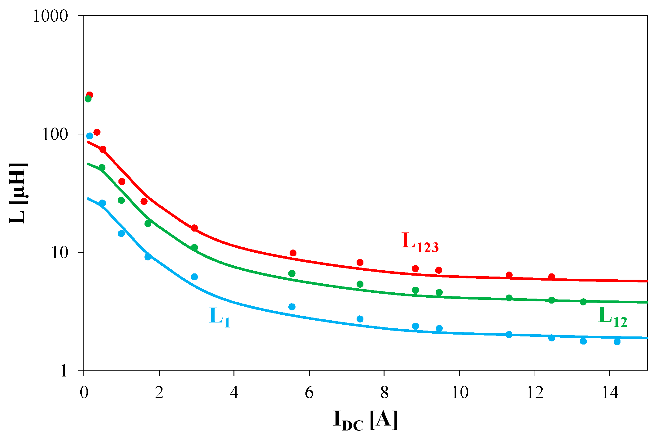
Figure 9 shows the dependence of inductance L
1 of a single winding, inductances of a series connected by two windings L
12, and inductances of a series connected by three windings L
123 of the coupled inductors on the direct current I
DC flowing through these coils at a frequency of the exciting signal equal to f = 200 kHz. The mentioned windings were wound on the same core.
The dependences L(I
DC) presented in
Figure 9 show that the results of the computations performed using the proposed model fit the results of the measurements very well in all the considered connections of the windings. It is also visible that in the case when two windings were connected in series, their inductance L
12 was over two-fold higher than inductance L
1 of the single winding. If three windings were connected in series, their inductance L
123 was over three-fold higher than inductance L
1. All the presented dependences L(I
DC) are monotonically decreasing functions.
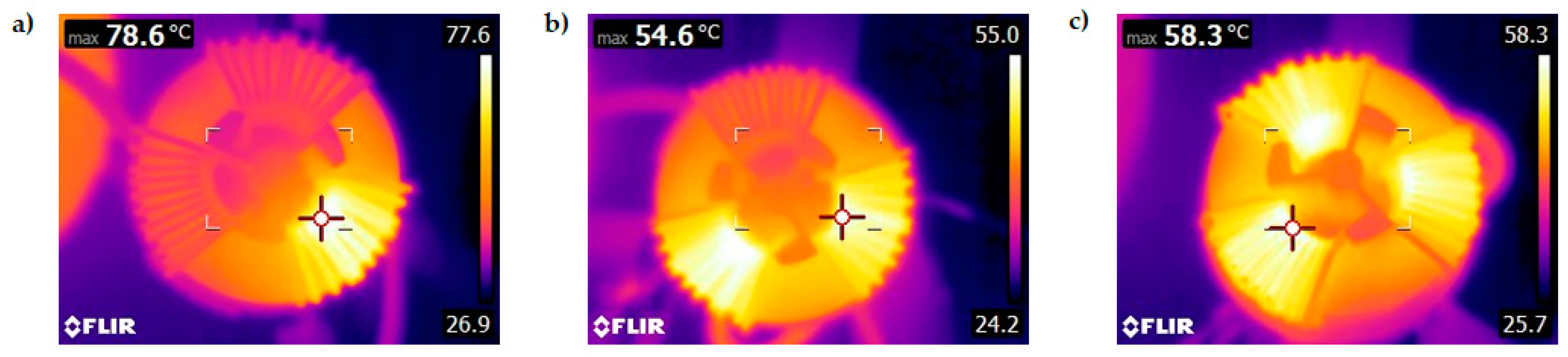
Figure 10 presents thermograms illustrating the temperature distribution in the investigated inductors when the current flowed through one winding (
Figure 10a), two windings connected in series (
Figure 10b), and three windings connected in series (
Figure 10c). In each of the considered cases, the power dissipated in one winding, two series-connected windings, and three series-connected windings was equal to 2.5 W.
It can be seen (
Figure 10) that the temperature distribution of the core and the winding was uneven and depended on the number of windings through which the current flowed. It can be noticed that when the current flowed through only one winding, the temperature TW1 of that winding reached up to 78 °C, and the temperature of the T
C core, resulting from thermal couplings between the core and the winding, reached approx. 45 °C and was almost 10 °C higher than the temperature of the other windings through which no current flowed. This proves that thermal coupling between the core and the winding was stronger than between the windings. On the other hand, when the current flowed through two or three series-connected windings, the temperature of such windings T
W12 and T
W123 was equal to 55 and 58 °C, respectively. It was also observed that the temperature of each winding through which the current flowed was the same. Additionally, it was observed that when the current flowed through two series-connected windings, the core temperature between the windings through which the current flowed was equal to 46 °C and was almost 5 °C higher than the temperature of the core near the winding through which the current did not flow. On the other hand, when the current flowed through three series-connected windings, the core temperature between all the windings was similar and was equal to 44 °C.
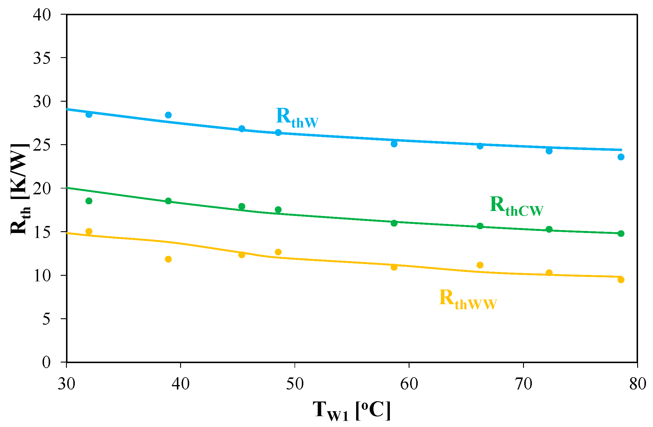
Figure 11 shows the dependence of thermal resistance of a single winding R
thW, thermal resistance between the core and winding R
thCW, and the mutual thermal resistance between the windings R
thWW on the temperature of this winding T
W1.
As can be seen, thermal resistance of the winding RthW, thermal resistance between the core and the winding RthCW, and mutual thermal resistance between the windings RthWW decreased with an increase in the first winding TW1 temperature, in which the power was dissipated. In each considered case, an increase in the winding temperature, in which the power was dissipated, of about 46 °C caused a decrease in the values of the mentioned thermal resistances by approx. 5 K/W.
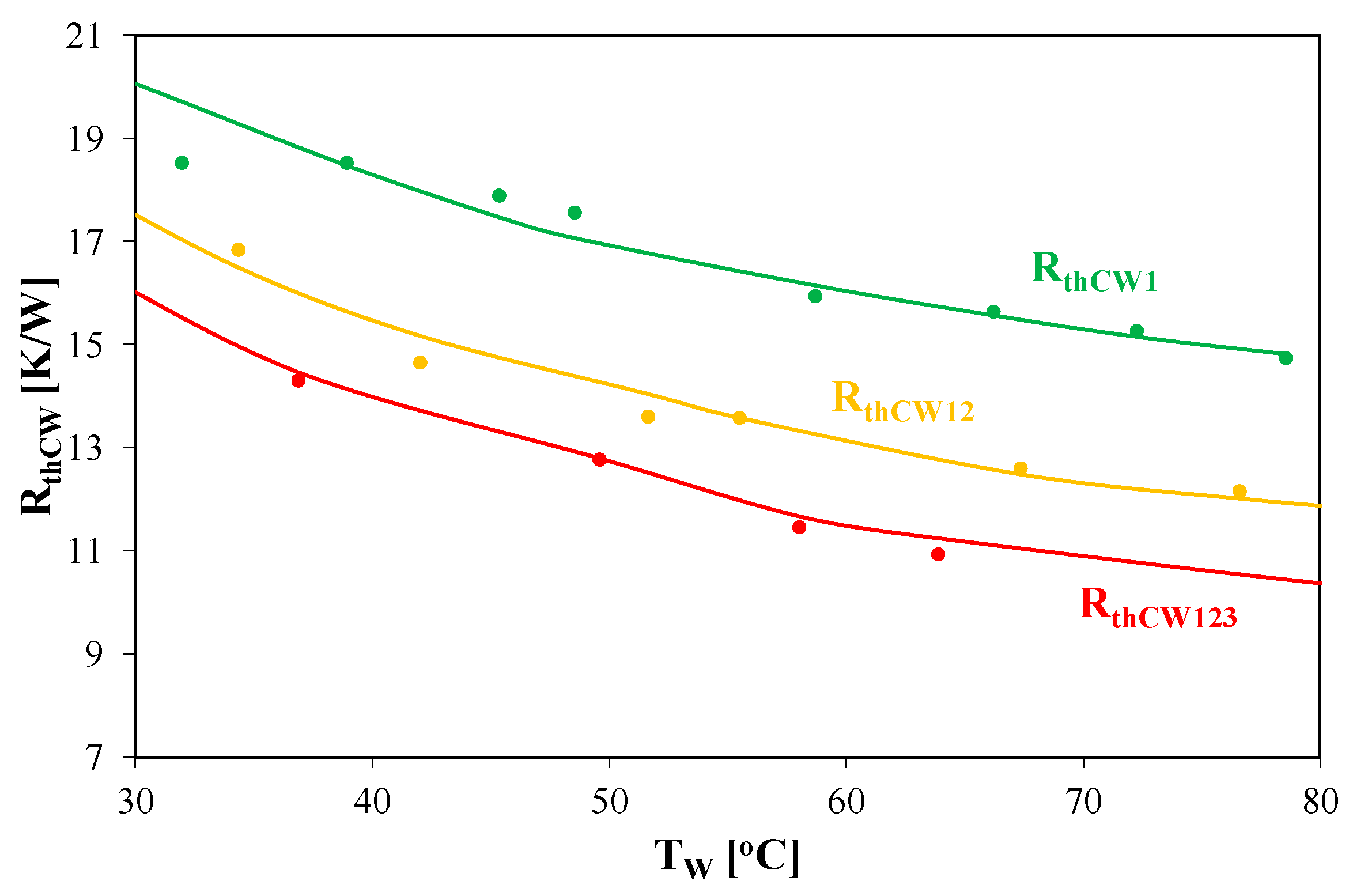
Figure 12 presents the dependence of mutual thermal resistances between the core and one R
thCW1, two R
thCW12, or three R
thCW123 windings on the winding, in which the power was dissipated.
As can be seen, the number of windings in which the power was dissipated significantly influenced thermal resistance of the inductor core. An increase in the number of windings in which the power was dissipated from one to three caused a decrease in the value of thermal resistance by up to 25%.
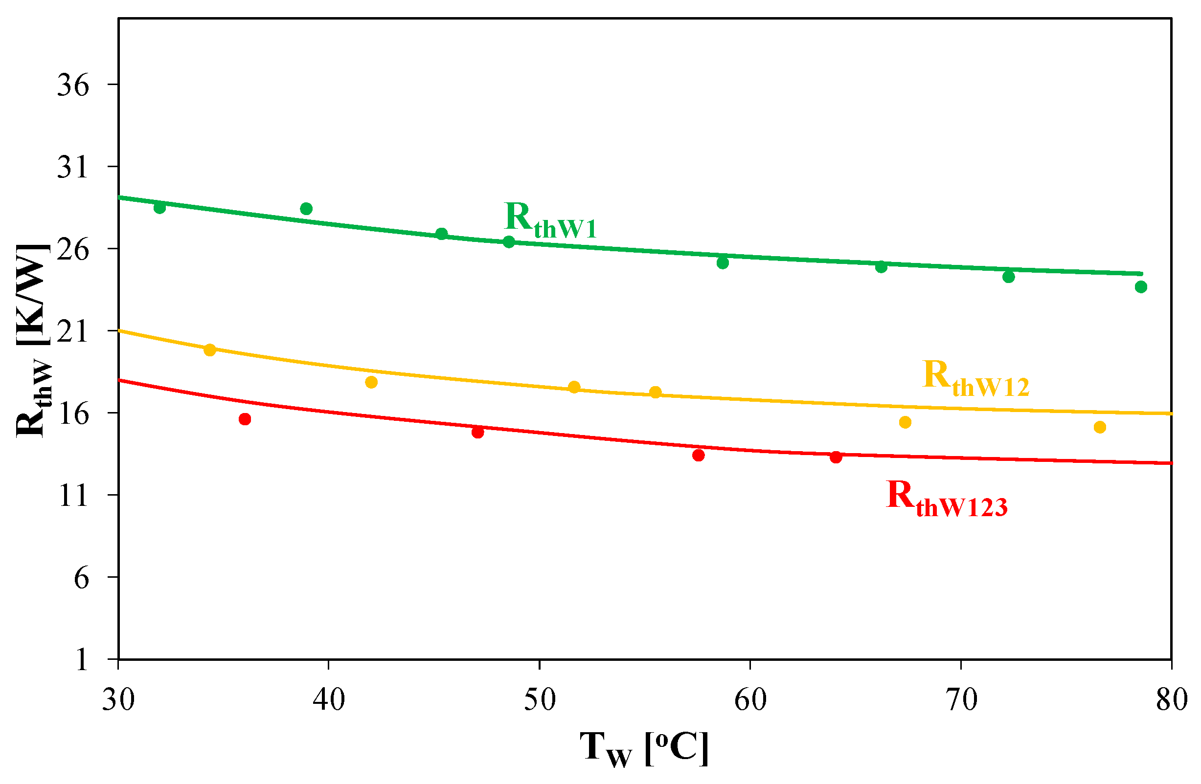
Figure 13 shows the dependence of thermal resistance of one R
thW1, two R
thW12, and three R
thW123 series-connected windings in which the power was dissipated on the temperature of these windings.
As in the case of thermal resistance of the core, the number of windings in which the power was dissipated significantly influenced thermal resistance of the inductor winding. An increase in the number of the mentioned windings from one to three caused a decrease in the value of thermal resistance RthW123 of the windings by up to 70% compared to RthW1.
Figure 14 shows the temperature dependence of all the inductor components on the direct current I
DC obtained when power was dissipated in one winding (a) and in three windings connected in series (b).
As can be seen in
Figure 14a, an increase in the direct current flowing through one winding L1 caused an increase in the temperature of all the components of the considered inductor as a result of mutual thermal interactions between the windings. An increase in the temperature of windings T
W2 and T
W3 at the direct current I
DC = 14 A was equal to 25 °C, whereas an increase in the core temperature T
C at I
DC = 14 A was equal to 33 °C. On the other hand, from the dependence shown in
Figure 14b, it can be seen that in the case of the power dissipated in three series-connected windings, the core and the winding temperature for I
DC < 6 A were the same. For I
DC > 6 A, the temperature of the winding was higher than the core temperature by about 10 °C.
This shows a strong thermal coupling between the components with increasing numbers of windings in which the power was dissipated. It should also be noted that the results of the calculations are in good agreement with the results of the measurements and the difference between the results of the calculations and measurements did not exceed 4%.
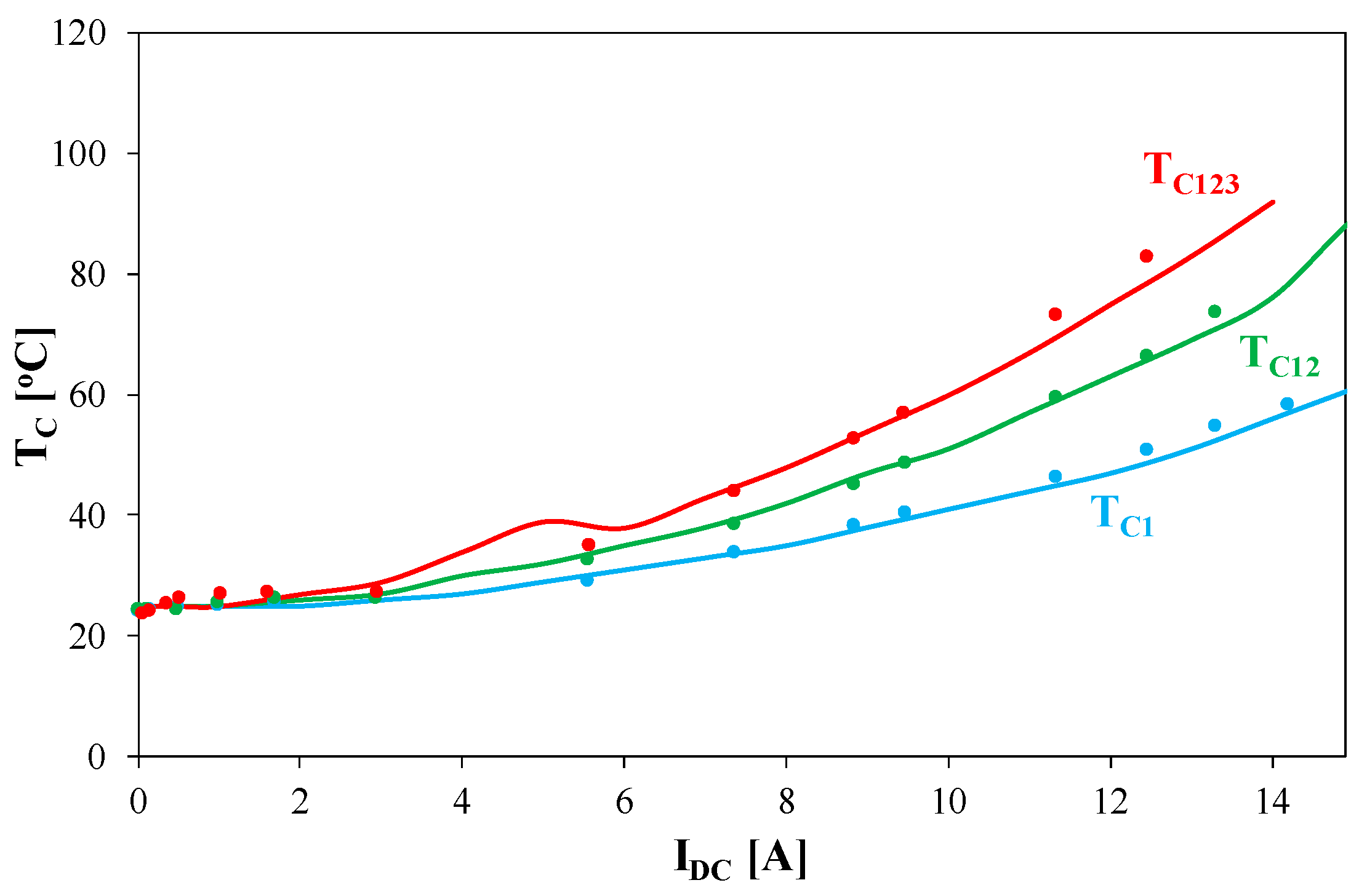
Figure 15 shows the dependence of the inductor core temperature on the direct current I
DC when the current flowed through one T
C1 winding, two series-connected T
C12 windings, and three series-connected T
C123 windings.
As expected, an increase in the number of windings in which power was dissipated caused a rise in the core temperature. In the case when the power was dissipated in only one winding, the temperature of the core T
C1 at I
DC = 14 A was equal to 59 °C. An increase in the number of windings in which the power was dissipated from one to three caused an increase in the temperature of T
C123 to almost 100 °C. As can be seen, the increase in the temperature of the inductor core with an increase in the number windings in which the power was dissipated was non-linear, which was shown in
Section 2. Additionally, it is worth noting that good agreement was obtained between the results of the calculations and measurements, and the difference between them did not exceed 5%.
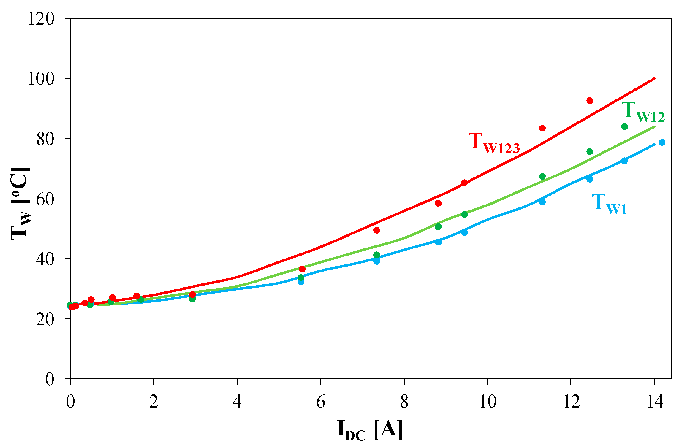
Figure 16 shows the dependence of the inductor winding temperature on the direct current I
DC obtained when the current flowed through one T
W1, two series-connected windings T
W12, and three series-connected windings T
W123. As can be seen, an increase in the number of windings in which the power was dissipated caused increases in the temperature of the inductor winding. It is observed that changes in the winding temperature with a change in the number of windings in which the power was dissipated had a non-linear character. If the current flowed through only one winding, the winding temperature at IDC = 14 A was equal to 78 °C. When the current flowed through three series-connected windings, the temperature of the winding TW123 exceeded 100 °C. Additionally, it is worth noting that the results of the measurements and calculations are in good agreement and the difference between them did not exceed 5%.
5.2. Characteristics of Coupled Inductor
The usefulness of the proposed electrothermal model of the coupled inductor in the analysis of switching systems was verified by calculating the influence of the load resistance on the output voltage. Additionally, the influence of the load resistance on the temperature of individual components of the coupled inductor operating in the boost converter was investigated. The analysed circuit is shown in
Figure 17.
In the considered circuit, a MOSFET transistor IRF540 (M1), a Schottky diode 1N5822 (D1), and passive elements R2 = 30 Ω and C1 = 50 µF were used. The resistor RL is the load of the converter, and the voltage source Vin is the power source. The signal Vp is a square wave generator with voltage levels equal to 0 and 10 V.
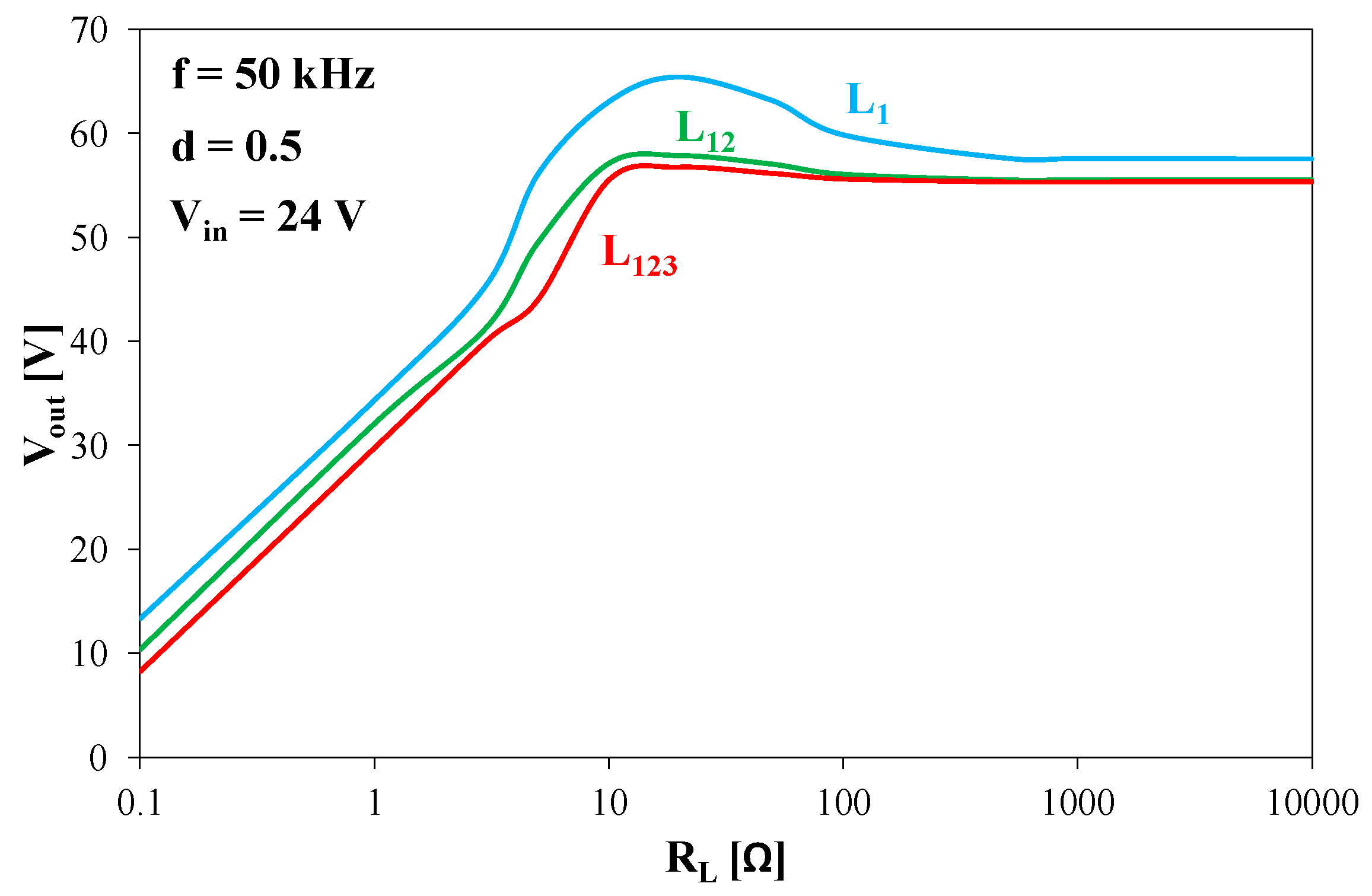
Figure 18 shows the calculated dependences of the output voltage of the considered converter on load resistance at the control signal frequency f = 50 kHz, the control signal duty cycle d = 0.5, and the value of the input voltage V
in = 24 V. The case of the current flowing through one winding L
1, two L
12 windings connected in series, and three L
123 windings connected in series was considered.
As can be seen, the dependence Vout (RL) had a local extreme at RL = 20 Ω when the current flowed through only one winding. In the case of the increasing number of windings in which the power was dissipated, this extreme shifted to the left side of the considered characteristic. It is also observed that an increase in load resistance RL from 0.1 to 10 Ω caused an almost seven-fold increase in the value of the output voltage Vout of the boost converter. On the other hand, at the load resistance RL > 100 Ω, the output voltage of the boost converter was constant. Additionally, an increase in the number of windings from one to three in which the power was dissipated reduced the value of the output voltage of the considered converter by over 10%. The maximum observed at RL equal to about 10 Ω is a result of the nonlinearity of the dependence L(i) of the inductor used. This dependence influenced the location of the border between the CCM and DCM modes.
Figure 19 shows the dependence of the core temperature T
C and the winding temperature T
W1, T
W2, and T
W3 of the coupled inductor operating in the boost converter on the load resistance. In this case, switches S
1 and S
2 were closed and the current flowed through only one coil L
1.
Figure 19 shows that an increase in the load resistance of the boost converter caused a decrease in the temperature of the core and all the windings of the coupled inductor. An increase was observed of the core temperature to T
C = 51 °C at R
L = 0.1 Ω and the temperature of the windings in which no power was dissipated at the same load resistance to T
W1 = T
W2 = 53 °C. This is the result of the strong thermal couplings between the windings and between the winding and the inductor core.


