Abstract
Considering the characteristics of narrow underground space and energy distribution, based on blade element momentum theory, Wilson optimization model and MATLAB programming calculation results, the torsion angle and chord length of wind turbine blade under the optimized conditions were obtained. Through coordinate transformation, the data were transformed into three-dimensional form. The three-dimensional model of the blade was constructed, and the horizontal axis wind turbine blade under the underground low wind speed environment was designed. The static structural analysis and modal analysis were carried out. Structural design, optimization calculation and aerodynamic analysis were carried out for three kinds of air ducts: external convex, internal concave and linear. The results show that the velocity distribution in the throat of linear air duct is relatively uniform and the growth rate is large, so it should be preferred. When the tunnel wind speed is 4.3 m/s and the rated speed is 224 rad/s, the maximum displacement of the blade is in the blade tip area and the maximum stress is at the blade root, which is not easy to resonate. The change rate of displacement, stress and strain of blade is positively correlated with speed. The energy of blade vibration is mainly concentrated in the swing vibration of the first and second modes. With the increase in vibration mode order, the amplitude and shape of the blade gradually transition to the coupling vibration of swing, swing and torsion. The stress and strain of the blade are lower than the allowable stress and strain of glass fiber reinforced plastics (FRP), and resonance is not easy to occur in the first two steps. The blade is generally safe and meets the design requirements.
1. Introduction
Coal resources are an important part of promoting China’s economic growth. With the economic development, the demand for coal resources in industrial production is increasing. However, the improvement of productivity and income has not successfully improved the safety monitoring level of mining enterprises, and the safety injury accidents of mining enterprises have not decreased with the progress of science and technology. According to the statistics of the national emergency management department, there were 123 coal mine accidents and 228 deaths in 2020. Especially since September 2020, three major coal mine accidents have occurred continuously in more than two months [1]. These accidents reflect that there are major omissions and problems in the implementation of government safety supervision and monitoring. How to ensure the safety of employees is not only the consistent requirement of the state, but also an important standard to measure the safety level of mining enterprises. As the first line of coal mining, underground working face is not only the area where underground workers work intensively, but also the area where gas, roof, accidental combustion and other injury accidents occur frequently. If the safety management problems of working face and mining area can be overcome, the number of mine accidents and deaths can be greatly reduced and the underground safety production level can be greatly improved [2].
In recent years, more and more wireless monitoring equipment and systems have been built in the underground roadway of coal mine to meet the increasing demand of coal mine safety monitoring [3]. However, different from the ordinary underground roadway of coal mine, the underground working face is an environment that develops dynamically with the mining progress. The wireless node can only run by the battery. Once the node is arranged, the battery cannot be replaced due to the poor environment, resulting in the short service life of the wireless network [4,5,6]. The core problem faced by the development of the energy supply system is to solve the energy supply. With the development of wireless sensor self-energy supply technology, this dilemma has gradually turned for the better. In particular, there is abundant and extensive energy underground, such as vibration energy generated by machinery, wind energy generated by ventilation, electromagnetic energy, heat energy, etc. [7,8]. The above energy is relatively stable, which provides prominent advantages for the design of wireless sensor self-energy supply system. If the above energy can be transformed into stable electric energy through technology to provide energy for the sensor system, it will greatly solve the dilemma faced by wireless sensors and is of great significance to the development of intelligent monitoring and unmanned working face [9]. By deploying a complete and comprehensive monitoring network underground, the safety level of the mine can be improved. The mine monitoring network is mainly responsible for monitoring various gas concentrations underground, including oxygen, carbon dioxide, carbon monoxide, methane, etc. [10]. At the same time, it also needs to monitor equipment operation status, mine ventilation, gas pressure, temperature, humidity and other environmental indicators. Various systems such as remote control of unmanned working face [11], sensor no blind area layout [12], and underground manual precise positioning technology need to ensure sustainable energy supply. The traditional wired energy supply mode shows many disadvantages, such as strong dependence on the line, high installation and maintenance cost of equipment and facilities, and even more seriously, if an accident occurs, the power supply line will be damaged, unable to provide relevant data support for subsequent search and rescue work. With the progress of internet of things mining technology, the micro wireless sensor system has been widely used in coal mining and mine safety monitoring [13]. However, due to the small volume of micro wireless sensor [14], its charged capacity cannot meet the needs of long-term work [15,16,17]. In actual mine application, the sensor deployment environment is complex, and personnel cannot directly reach the location of the sensor to replace the battery, as a result, the availability of sensor network in mine is reduced. Therefore, collecting energy from the surrounding environment of the coalmine, realizing the self-energy supply of wireless sensors, continuously supplying power to sensor nodes, and improving the sustainability and stability of wireless sensor networks are the key to solving the life limitation of wireless sensor networks.
As a renewable and clean energy, wind energy is widely distributed in China [18,19,20]. Wind power generation is the main form of wind energy utilization. As the core component of wind power generation system, the structure of blades determines the utilization rate of wind energy [21,22,23]. In recent years, with the reduction in wind farm construction sites and the promotion of distributed energy, the development speed of small wind turbines is gradually accelerating. How to optimize the blade structure design of small wind turbines and improve the power generation efficiency of wind turbines has become a research hotspot [24]. FloDesign [25], located at the American Institute of Aeronautical Engineering, has developed a wind turbine structure superior to the traditional wind turbine. The system arranges sunshades around the wind turbine blades to guide the air to increase the movement through the impeller, accelerate the wind flow and improve the power of the wind turbine. The principle of the wind turbine model is as follows: after the wind flow enters the wind turbine, under the guidance of fixed blades on one side, it flows to the blades on the other side at a specific angle to ensure that the wind flow can achieve the maximum efficiency, and then promote the rotation of the wind turbine. At the same time, the streamlined shelter can accelerate the air with high velocity outside the wind turbine, drain it to the rear of the wind turbine, and form a static pressure zone at the front end of the blade, and can make more air flow in. In particular, MIT experts believe that this system may increase production capacity many times. The research institute has produced a prototype for larger wind tunnel tests, with the goal of evaluating its diameter of 3.66 m and performance of 10 kW. Ohya et al. [26] in Japan have been studying and trying to manufacture light wind turbines with the best operation effect in low wind speed areas for a long time. The research project is tested with a 500 W wind turbine. The production coefficient of the prototype set a record of 1.4, indicating that the efficiency of the power generation device can reach five times that of the general wind turbine. The diversion device of Chen [27] in Germany has made some innovations in the wind turbine design system. In order to improve the utilization rate of wind energy, a blade is set at the inlet and outlet ends of the wind turbine, a large four blade is set at the inlet end, and a small five blade is set at the outlet. In this way, due to the blocking effect of wind flow through two impellers, wind speed can be greatly utilized. Dena Hendriana et al. [28] optimized the wind turbine by changing the blade inclination and width, and found that the change of wind speed will affect the maximum power of the wind turbine. C. M. Chan and others [29] discussed the optimal blade performance of the Savonius wind turbine based on a genetic algorithm, and studied the turbine aerodynamic and fluid structure under different blade shapes. Ramazan and Mustafa used non-dominated sorting genetic algorithm to optimize the blade structure of wind turbine and improve the working efficiency of small wind turbine [30]. Zhu et al. [31] optimized the overall performance of wind turbine blades based on MATLAB and ANSYS numerical software, and verified the rationality of the designed blades with an example. In addition, some scholars use bionics [32] and neural network method [33] to optimize the external structure of small wind turbine blades. The above research on small wind turbine blades has made great progress. However, in addition to the structural design of wind turbine blades, the wind turbine rotor area, air density and installation location are closely related to the power generation efficiency of wind turbine. Therefore, it is still uncertain whether the structural design optimization of small wind turbine blades under specific conditions is applicable to all areas. For example, the wind speed in the coalmine is low, the space is small and the ventilation network is complex. When the wind turbine is installed in the roadway, the designed blades are unreasonable. On one side, it is very easy to cause airflow short circuit and insufficient air supply in the working face, resulting in disasters. On the other hand, the blades cannot capture more wind energy, resulting in low power generation efficiency of wind turbines, unable to provide sufficient energy, resulting in a waste of resources.
Great progress has been made in the above research on small wind turbine blades. However, in addition to the structural design of wind turbine blades, the wind turbine wheel area, air density and installation location are closely related to the power generation efficiency of wind turbine. Therefore, whether the structural design optimization of small wind turbine blades under specific conditions is suitable for all areas is still uncertain. For example, the wind speed in the coal mine is low, the space is small and the ventilation network is complex. When the wind turbine is installed in the roadway, the designed blades are unreasonable. On the one hand, it is very easy to cause air flow short circuit and insufficient air supply in the working face, resulting in disasters. On the other hand, the blades cannot capture more wind energy, resulting in low power generation efficiency of wind turbines, unable to provide sufficient energy, resulting in a waste of resources.
Underground wind energy widely exists in various roadways and shafts, and is relatively stable. It is an excellent energy supply source [34]. It can convert the air flow in the roadway into stable electricity, which can not only reduce the pressure of coal mine power supply station, but also provide good technical support for the development of coal mine intelligence. At present, most mines mainly rely on thermal power and methane power generation to supply underground equipment [35]. For wind power generation, there are few reports on the realization of mine wireless sensor self-energy supply [36].
This paper aims to design a self-powered, flexible networking and reliable micro wind power generation system, focus on the design of wind tunnel wind turbine, study its structural performance, and make a comprehensive analysis, so as to provide suggestive guidance for establishing a more perfect mine self-energy supply sensor network in practical application. In view of this, the spatial coordinate system of blade is established based on coordinate transformation theory, the actual three-dimensional spatial coordinates of discrete points of each blade element are solved, and the three-dimensional model of the blade is established through SoildWorks. Taking the wind speed conditions of the main air inlet roadway of the coal mine as the reference, the static structure analysis and modal analysis of the wind turbine blade are carried out by using ANSYS Workbench software, so as to provide technical support for the practical application of the small air duct horizontal axis wind turbine in the mine.
2. Air Duct Design
2.1. Influence Analysis of Breeze Power Generation System on Underground Ventilation System
In the underground ventilation, the pipes, electric locomotives, cages and tank way beams in the roadway will form a certain blocking effect on the air flow. Due to its blocking effect, the air flow will quickly change the wind speed and direction. After the air flow is redistributed, a damage field and eddy current area will be formed behind the equipment, and wind energy loss will be generated. In the roadway, due to the continuous operation of the fan and sufficient air volume, these resistances are usually small, but they should also be checked and calculated in the design.
Assuming that the wind turbine is an entity, the front resistance generated by the installation of the wind turbine is calculated. The calculation formula and analysis of the front resistance of the wind turbine prove the following relationship theoretically and experimentally [37]:
where is front resistance, Pa; C is frontal resistance coefficient, dimensionless; S is roadway sectional area, m2; is projected area of front resistance object; Sm is perpendicular to the general direction of air flow, m2; Vm is average speed of air flow passing through the empty section (S − Sm) of the roadway, m/s; ρ is air density, kg/m3.
The front resistance coefficient C of the wind turbine is a coefficient only related to the total length of the wind turbine, the cross-sectional area of the wind turbine, the structural form of the windward end of the wind turbine and the roadway section parameters. When the wind turbine and roadway parameters are certain, its C value should be a constant, regardless of the air volume passing through the roadway. So according to Vm = , where q is roadway air volume, m3/s; it is deduced that:
Because under specific conditions, C, S, Sm, ρ are constants, so we can make:
Rc in the formula is called the front wind resistance of the wind turbine, N·s2/m8. According to previous experience [38], ≈ 0.010959 N·s2/m8.
The above formula shows that the front resistance of wind turbine is equal to the product of its front resistance and the square of roadway air volume, which has the general formula form of resistance law. Through calculation, the wind turbine is installed underground and will not affect the ventilation and safety of coal mine. Therefore, it complies with coal mine safety regulations. Since it is a micro wind turbine, its size, volume and power are very small, which has little impact on the additional resistance in the air supply system and the additional energy cost of the fans. There is no need to rebuild the existing air supply systems of the mine.
2.2. Design Theory
The air duct in this design is the external air duct structure of small horizontal axis wind turbine, as shown in Figure 1. The energy accumulation principle of the air duct can be obtained from the analysis of fluid continuity equation.
where CT is the torque coefficient, ρ is the air density, S is the coverage area of the wind turbine impeller, R is the radius at the section; and U∞ is the wind speed flowing into the cross section of the wind turbine impeller.
where ρ is the air density, S is the coverage area of the wind turbine impeller, CP is the power coefficient, and U∞ is the wind speed flowing into the cross section of the wind turbine impeller.

Figure 1.
Structure of external air duct of horizontal axis wind turbine.
In this paper, the incompressible fluid model is adopted. According to the continuity equation of fluid, it can be seen that:
where , is the wind speed at the inlet of the air duct and the throat (at the impeller of the wind turbine); S1 is the cross-sectional area of air duct inlet; S2 is the cross-sectional area of the throat of the air duct.
2.3. Shape Design of Air Duct
In order to gather more wind energy and accelerate the air flow, the air duct structure should be designed according to the area of the air inlet greater than the air outlet. In addition, while accelerating the air flow, the relationship between the shape of the air duct and the wind acceleration effect should be considered, so as to select the optimal structural parameters. Now, the following three schemes are designed according to the functional shape of the air duct, which are convex, concave and linear, as shown in Figure 2.
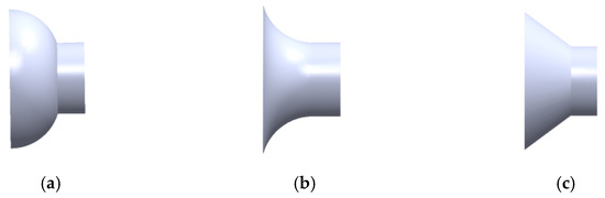
Figure 2.
Schematic diagram of three types of air duct shapes: (a) Convex type; (b) Concave type; (c) Linear type.
2.4. Numerical Calculation of Three Schemes of Air Duct
In order to compare and analyze the air collection effects of the three schemes, the three air duct models are simulated by FLUENT software. In order to ensure the reliability of the calculation results and facilitate comparative analysis, the basic initial conditions such as size and flow field environment are the same in the three schemes. For the convenience of calculation, the flow field is simplified as only a single wind speed perpendicular to the inlet. The uniform size of air duct is the area of air inlet and outlet is the same. The diameter of the air inlet is 0.42 m and the diameter of the air outlet is 0.21 m. The length of the rectifier tube is the same, the length of the air duct is 0.08 m, and the axial length of the air duct is 0.14 m.
The structural grid is selected as the grid type. In order to improve the calculation accuracy, the air duct and outer watershed are defined, respectively, and the grid density near the air duct is increased. The total number of grids is 991,897 and the number of nodes is 1,063,143, as shown in Figure 3. Considering the coupling effect of air duct and incoming flow, the three-dimensional steady-state solution is calculated by using the implicit solver based on pressure. In order to improve the convergence speed and calculation accuracy, the velocity pressure coupling algorithm is adopted, the smaller relaxation factor is selected, and the Second-Order Upwind scheme is selected.

Figure 3.
Grid division of three schemes: (a) Grid division of linear air; (b) Grid division of outer convex air; (c) Grid division of inner concave air.
2.5. Analysis of Calculation Results and Scheme Selection
Figure 4, Figure 5 and Figure 6 show the velocity distribution cloud maps of linear, convex and concave air ducts, respectively. Figure 7 and Figure 8 show the velocity variation curves of inlet and throat of three air ducts. Figure 9 shows the distribution of blade chord length along radius, which is optimized by using MATLAB software. As can be seen from Figure 4, Figure 5, Figure 6, Figure 7, Figure 8 and Figure 9:
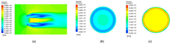
Figure 4.
Cloud map of velocity distribution of linear air duct: (a) Cloud map of velocity distribution in air duct basin; (b) Inlet velocity distribution cloud map; (c) Velocity distribution cloud map of throat.

Figure 5.
Cloud map of velocity distribution of external convex air duct: (a) Cloud map of velocity distribution in air duct Basin; (b) Inlet velocity distribution cloud map; (c) Throat velocity distribution cloud map.

Figure 6.
Cloud map of velocity distribution of concave air duct: (a) Cloud map of velocity distribution in air duct basin; (b) Inlet velocity distribution cloud map (c) Velocity distribution cloud map of throat.

Figure 7.
Inlet velocity variation curves of three kinds of air ducts.

Figure 8.
Throat velocity curves of three kinds of air ducts.

Figure 9.
Blade chord length distribution along the radius.
- Inlet velocity analysis: according to the inlet velocity distribution cloud map of the three schemes, the inlet velocity of the three schemes is 3 m/s lower than that of the external flow field, indicating that the air duct has a certain blocking effect on the incoming flow. Due to the high internal wind speed and higher pressure than the outside, the inlet air flow cannot completely enter the air duct, and the air duct will form a certain blocking effect on the incoming flow. In the scheme of linear air duct, the central velocity is large, which is 2.0 m/s. with the increase in radius, the velocity decreases to 1.1 m/s, and then increases to 2.6 m/s. The variation trend of the velocity of the outer convex and inner concave air duct with the radius is basically the same as that of the linear air duct. The central velocity is large, and the velocity decreases with the increase in the radius. The central velocity of the outer convex air duct is 1.5 m/s and that of the inner concave air duct is 2.15 m/s.
- Throat velocity analysis: according to the throat velocity distribution cloud maps of the three schemes, in the linear air duct scheme, the overall color of the section is yellow and the velocity distribution is uniform. The color of the central area of the outer convex air duct is orange, and the basic color of the surrounding ring is red, indicating that the velocity at the center is smaller than that of the surrounding ring, and the velocity distribution is uneven. The overall color of the concave air duct is red, and the velocity distribution is relatively uniform.
- It can be seen from the comparison between the outer convex and inner concave schemes that the velocity at the center of the outer convex air duct is large (Figure 5a), occupies most of the area of the outlet, and the maximum area of velocity distribution is about 4.2 m/s. The velocity at the center of the concave air duct is small (Figure 6a), about 3.90 m/s, and the velocity at the outer ring is about 4.0 m/s. The velocity distribution increases along the radial direction of the circle, which will have a certain impact on the safety of the blade. As shown in Figure 9, the thickness change of the front section of the blade first increases and then decreases along the radial direction. The thickness at the blade tip is the smallest, but at this time, the wind speed is the largest, and the safety of the blade will decline rapidly.
Figure 10, Figure 11 and Figure 12 show the pressure distribution cloud maps of the three schemes. It can be seen from Figure 10, Figure 11 and Figure 12 that the external convex air duct bears the maximum force, and the pressure on its wall reaches about 11.2 Pa. The stress surface of linear air duct and internal concave air duct is small, about 10 Pa. At the same time, it can be observed that the inlet edge of the concave air duct is particularly affected by the airflow resistance and serious energy loss, which is one of the reasons for the low throat velocity. Therefore, considering the throat velocity and the pressure on the air duct, the optimal shape of the air duct is linear, which will be used as the basis of subsequent design.
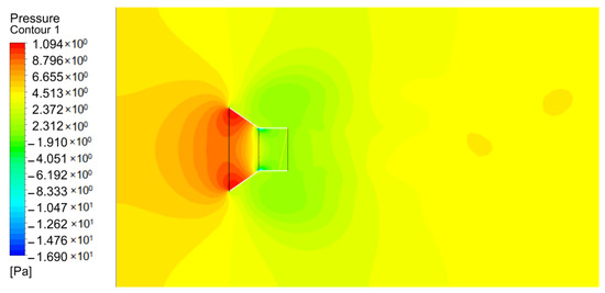
Figure 10.
Cloud map of linear pressure distribution.
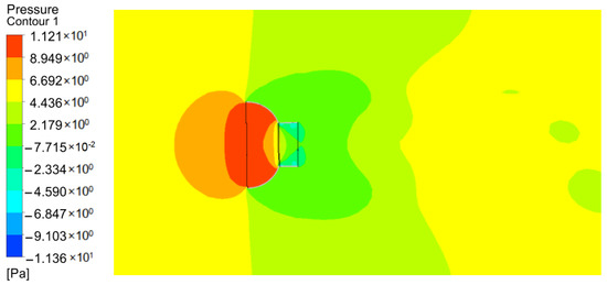
Figure 11.
Cloud map of convex pressure distribution.
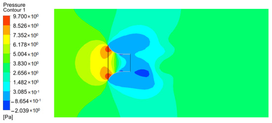
Figure 12.
Cloud map of concave pressure distribution.
2.6. Effect of Expansion Angle on Wind Speed Amplification Performance of Linear Air Duct
In Section 2.4, the linear air duct is selected as the optimal shape, so study of the influence of different expansion angles on the wind speed amplification performance of the linear air duct continues. The linear air ducts with expansion angles of 10°, 15°, 20°, 30°, 37°, 40° and 50° are selected for simulation calculation, and the velocity differences of different expansion angles are compared. At the same time, all models set the inlet wind speed of the flow field as 3.0 m/s, and other parameters remain unchanged. Figure 13 shows the acceleration ratio curve of different expansion angles. The data shown in Figure 13 is obtained by numerical simulation using FLUENT software. It can be seen from Figure 13 that the acceleration ratio of the air duct first rises to the peak and then decreases with the increase in expansion angle. When the expansion angle is 37°, the maximum growth ratio is 1.45. This is because with the change of expansion angle, the flow field near the draft tube will change greatly. When the expansion angle is 37°, the acceleration ratio reaches the peak. With the expansion of expansion angle, the flow field outside the draft tube appears when the expansion angle is 40°, and the flow is more obvious when the expansion angle is 50°. This flow around will lead to high internal wind pressure, and the air flow can no longer enter the air duct, so the internal wind speed of the air duct will decrease rapidly. According to the above research, when the expansion angle is 37°, it cannot only ensure that the air duct has a high acceleration ratio, but also ensure the stability of the flow field near the air duct. Therefore, the most preferred type of air duct is linear, and the expansion angle is 37°.

Figure 13.
Curve of acceleration ratio with different expansion angles for linear air duct.
3. Blade Design of Horizontal Axis Wind Turbine
3.1. Leaf Element Momentum Theory
Leaf element momentum theory combines leaf element theory and momentum theory. Its basic idea is to divide the blade into finite element leaf elements along the leaf span direction. Integrating leaf element theory and momentum theory, the relationship between tangential and axial induction factors and torsion angle and leaf element chord length can be expressed as [39]:
where a is the axial induction factor. b is tangential inducer. N is the number of blades. C is the chord length of leaf element section. CL is the lift coefficient. CD is the resistance coefficient. φ is the inflow angle. R is the radius.
3.2. Wilson Optimization Mathematical Model
3.2.1. Wilson Model
Based on the Glauert method, Wilson studied the Glauert method and analyzed the effects of tip loss and lift drag ratio on blade performance
The local optimal power coefficient of the blade can be described as [40]:
where CP is the local optimal power coefficient of the blade. F is Prandtl correction factor. λ is the corresponding tip speed ratio at blade spread r.
In order to maximize the local optimal power coefficient, the following constraints are given:
The Prandtl correction factor can be expressed as:
The inflow angle can be expressed as:
The calculation formula of blade chord length is:
where α is the angle of attack.
3.2.2. Wilson Model Optimization Steps
- Based on the blade element momentum theory, the blade of the wind turbine is divided into several equal parts along the spanwise direction;
- Analyze the optimization problem of each leaf element, take Equation (8) as the objective function and Equation (9) as the condition function, and calculate the interference coefficients a, b and Prandtl correction factor F of each leaf element;
- According to Equations (11)–(13), the inflow angle, the torsion angle of each blade element and the chord length can be obtained, respectively;
- The chord length and torsion angle calculated above are linearly corrected to meet the requirements of structure and easy fabrication;
- According to the airfoil data, the airfoil coordinates of each blade element are calculated.
3.2.3. Flow Chart of Blade Optimization Design
The nonlinear constrained optimization function fmincon in MATLAB is used to optimize the chord length and torsion angle of each blade element, and the optimal wind turbine blade structural parameters are designed by combining the blade geometry and program programming.
The optimized mathematical model is:
Objective function:
Constraint function:
MATLAB optimization calculation flow chart, as shown in Figure 14.

Figure 14.
MATLAB optimization calculation flow chart.
3.2.4. Chord Length and Torsion Angle Correction
Combined with MATLAB programming and Wilson optimization design, 20 sections of the blade are optimized to obtain the torsion angle and chord length under the optimization conditions of each section. The operation calculation results are shown in Table 1.

Table 1.
MATLAB optimization and fitting results.
3.2.5. Airfoil Design
The working condition of the wind turbine designed in this paper is low Reynolds number, but the traditional airfoils, such as NACA and NASA series, are mainly suitable for high Reynolds number (Re > 5 × 10⁶) or medium Reynolds number (5 × 10⁵ < Re < 3 × 10⁶); if these airfoils are applied to low Reynolds number (Re < 5 × 10⁵), laminar flow separation will occur, so low Reynolds number airfoils must be used on wind turbines. Four typical NACA5505, BW-3, SG6043 and A18 airfoils [41] are selected from the “low speed airfoil data summary”, and the airfoil types are shown in Figure 15.

Figure 15.
Dimensionless diagram of four low Reynolds number airfoils relative to chord length.
The optimal airfoil is selected by analyzing the lift drag ratio, thrust coefficient and surface stability of four typical airfoils at low Reynolds number. Since the lift coefficient Cl and drag coefficient Cd are functions of angle of attack ∂ and Reynolds number Re, it is a prerequisite to determine the appropriate Reynolds number; according to the Reynolds number calculation formula, the Reynolds number of the designed micro wind turbine is about 2 × 10⁴ [42]. Figure 16, Figure 17 and Figure 18 show the aerodynamic characteristic curves of four typical airfoils under Re = 2 × 10⁴.

Figure 16.
Relation curve between lift Cl and drag Cd of blade airfoil.
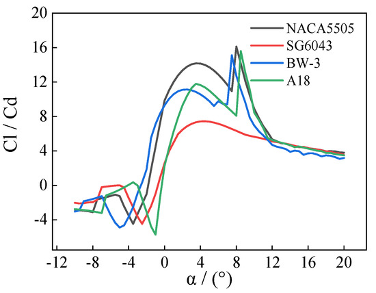
Figure 17.
The relationship curve between the lift-drag ratio Cl/Cd of the blade airfoil.

Figure 18.
The relationship curve between blade airfoil moment coefficient Cm and angle of attack α.
It can be seen from Figure 16, Figure 17 and Figure 18 that the NAC5505 airfoil has a high lift-drag ratio and stability at low Reynolds number, so NACA5505 airfoil is selected as the design airfoil, the best angle of attack α = 8°, and the lift-drag ratio Cl/Cd is 16.12, Cl = 1.2329, Cd = 0.0765. Due to the low velocity of the mine roadway (1.5–8 m/s), a low Reynolds number airfoil (Re = 2 × 10⁴) must be used, so NACA5505 airfoil is selected as the design airfoil. The airfoil is shown in Figure 19.

Figure 19.
Dimensionless schematic diagram of NACA5505 airfoil.
3.2.6. Three Dimensional Model of Blade
Based on the obtained parameters such as chord length and torsion angle of each leaf element, the actual spatial coordinates of each leaf element of the blade are calculated through the spatial transformation of coordinate points. Finally, the data are imported into SoildWorks to generate the geometric surface of the blade in batch and establish the three-dimensional model of the blade. The three-dimensional model is shown in Figure 20.
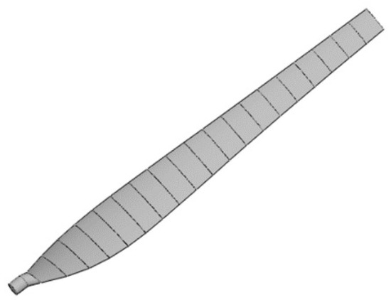
Figure 20.
Three-dimensional model of blade.
3.2.7. Initial Parameter Design of Wind Turbine
Wind Speed Design
Underground wind energy is more reliable than natural wind, with an average wind speed of 3.5 m/s and a maximum wind speed of 8 m/s. However, due to the changing underground structure and characteristics, wind energy has volatility and uncertainty. At the same time, the distribution of wind speed in the shaft section is uneven, because the wind flow is viscous and has friction with the shaft wall. Therefore, the wind speed is the maximum at the central axis of the shaft, gradually decreases along the radial wall, and reaches the minimum at the wall. The whole is distributed in a parabola shape and symmetry.
The change rate of wind speed in the radial direction is mainly related to the roughness of the shaft wall. The greater the surface roughness of the shaft wall, the greater the change rate of wind speed. The change rate of wind speed is generally expressed by the speed coefficient kv.
where vavg is the average wind speed, m/s; vmax is the maximum wind speed, m/s.
With the continuous improvement of well construction technology, the surface of shaft wall has been relatively smooth. According to literature [43], the shaft velocity field coefficient is generally about 0.9, and the shaft diameter is large (5–10 m), so the wind speed at the shaft section can be regarded as uniform distribution in power generation calculation.
From the above analysis, it can be concluded that there is wind energy with high wind speed and uniform distribution in the roadway environment for a long time, which can provide a stable energy source for the energy collection device. Therefore, the incoming wind speed of the designed mine air duct horizontal axis wind turbine is 3 m/s. From the above analysis, it can be concluded that there is wind energy with high wind speed and uniform distribution in the roadway environment for a long time, which can provide a stable energy source for the energy collection device. Therefore, the incoming wind speed of the horizontal axis wind turbine with mine air duct is designed to be 3 m/s. According to Equations (4) and (5), under the action of wind flow, the output torque T of wind turbine is directly proportional to the square of impeller wind speed u∞, and the output power P is directly proportional to the third power of impeller wind speed u∞. Through the wind turbine, the wind speed entering the impeller can be increased to 1.5 times the original wind speed. Therefore, the design wind speed at the front end of the blade is about 4.3 m/s.
Blade Radius Design
It can be seen from the above design that the wind speed of the design duct is accelerated from 3 m/s to 4.3 m/s, and the ratio of the inlet and throat of the air duct is 2:1. Considering the special underground environment and roadway area, the space of wind turbine can be preset. The design inlet diameter is 0.42 m, the design throat diameter is 0.21 m, the blade radius is 0.1 m and the hub radius is 0.005 m. The size of the designed air duct is shown in Figure 21.
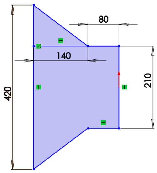
Figure 21.
Dimensions of air duct.
Rated Power Design of Wind Turbine
The rated power of wind turbine can be seen from formula [44]:
where P is the rated power of fan, W; ρ is the air density, taken as 1.225 kg/m3; CP is the utilization coefficient of wind energy, taken as 0.4; A is the swept area of impeller, A = πR2, taken as 0.0314 m2; η1 × η2 is the product of transmission efficiency and electric efficiency, taken as η1 × η2 = 0.9; V is the wind speed at the front end of the blade, taking the wind speed of 4.3 m/s. From the formula, P = 0.482 W.
Design of Tip Speed Ratio and Blade Number
Calculation formula of tip speed ratio:
According to the tip speed ratio theorem, Equation (18) is applicable to wind turbine blades with stable wind speed. According to Equation (18), the smaller the tip speed ratio, the higher the angular velocity of the impeller. Theoretically, the higher the wind speed, the higher the power generation performance of the wind turbine. Generally speaking, the speed of large wind turbines is usually low. Under the same power output, small wind turbine has higher rated speed to ensure greater energy conversion efficiency. The tip speed ratio is usually 4–8. The tip speed ratio is determined by Table 2.
Table 2.
Matching between tip speed ratio and blade number.
The wind turbine studied in this paper is a micro wind turbine. High speed is selected to ensure a certain wind energy utilization rate λ0 = 4. When λ0 = 4, the number of blades can be taken as 3~5. Because the five blade wind turbine is more stable in operation and power output than the three blade wind turbine, at present, most micro wind turbines at home and abroad use five blades, so the number of blades of the wind turbine is N = 5.
4. Blade Structure Performance Analysis
Static structural analysis and modal analysis are the two key analysis directions of blade structural performance analysis. In this paper, the three-dimensional model is imported through the structural analysis software ANSYS Workbench to carry out static structural analysis and modal analysis, so as to verify whether its structural performance meets the safety requirements. FRP is selected as the blade material, which has the characteristics of high strength and lightweight. Table 3 shows the relevant material properties of FRP materials.
Table 3.
Characteristics of selected blade materials.
4.1. Geometric Model and Boundary Conditions
Import the step format wind turbine file established by SoildWorks into meshing. The number of grid units is 141,191, and the total number of nodes is 178,723. The blade radius is 0.1 m, and the number of blades is five. The established three-dimensional wind turbine blade model and grid division diagram are shown in Figure 22.

Figure 22.
Grid division diagram of blade.
Boundary condition: constraint condition and static load are the two most important aspects. The constraint condition is to restrict and fix the blade root, that is, the blade constraint is simplified into cantilever beam form. The static load mainly includes: the load generated by the blade’s own gravity and the load generated by aerodynamic force, including shear force, tensile pressure, bending and torsional moment, etc. In the boundary condition setting, the inertial force is used to represent the gravity load, and the aerodynamic load is evenly distributed on the blade surface.
4.2. Simulation Results of Blade Static Structure
According to the coalmine safety regulations, the maximum wind speed of the main air inlet roadway shall not exceed 8 m/s, and the average actual mine wind speed is generally 3.5 m/s. Therefore, the design wind speed at the front end of the blade is about 4.3 m/s. under the load of rated speed 224 rad/s, the cloud maps of displacement, stress and strain of the blade are shown in Figure 23, Figure 24 and Figure 25 when the incoming wind is 4.3 m/s.
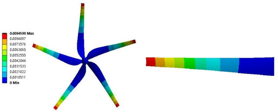
Figure 23.
Cloud map of blade displacement.
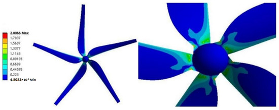
Figure 24.
Stress cloud map of blade.

Figure 25.
Cloud map of blade strain.
Figure 23, Figure 24 and Figure 25 show the displacement, stress and strain cloud maps of the blade. The following conclusions can be drawn from Figure 23, Figure 24 and Figure 25:
- The overall displacement of the blade is small and increases gradually along the radial displacement of the blade. The maximum displacement change occurs at the blade tip, the maximum displacement is 0.00946 mm, and the displacement at the blade root is small;
- The maximum stress and strain of the blade is located at the root of the blade, and the maximum stress is 2.07 MPa. The stress in the overall area of the blade surface is relatively small, which is 4.8083 × 10⁻⁵ MPa. The stress and strain are lower than the allowable stress and strain of FRP material. The blade structure is safe and meets the design requirements.
4.3. Static Strength Analysis of Blades under Different Working Conditions
The static strength stability of blade under different working conditions is analyzed by changing different rotating speeds. The variation law of blade displacement, stress and strain with rotating speed under the conditions of 100 rad/s, 200 rad/s, 300 rad/s, 400 rad/s and 500 rad/s is studied, as shown in Figure 26, Figure 27 and Figure 28.

Figure 26.
Displacement curve at different speeds.
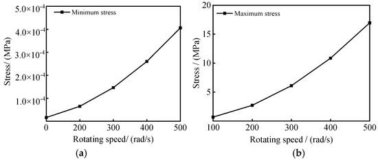
Figure 27.
Stress curve of blade at different speeds: (a) Minimum stress curve; (b) Maximum stress curve.

Figure 28.
Blade strain curve at different speeds: (a) Minimum strain curve; (b) Maximum strain curve.
As can be seen from Figure 26, Figure 27 and Figure 28, the displacement, stress and strain of the blade increase with the increase in rotating speed. When the rotating speed is low (100–300 rad·s−1), the incoming wind speed plays a leading role, and the change rate of blade displacement, stress and strain is small. With the increase in rotating speed, the change rate of blade displacement, stress and strain increase. When the rotating speed is 500 rad·s−1, the maximum displacement of the blade is 8 cm, The maximum stress is 16.957 MPa and the maximum strain is 8.90 × 10⁻⁵, the safety factor of the blade is reduced to 14.743, and the structural stability of the blade is slightly loose, but it is still within the controllable range, meeting the design requirements.
4.4. Blade Modal Analysis
4.4.1. Wilson Model
Under the action of external force, the differential equation of blade motion is:
where [M] is the mass matrix of the blade; is the acceleration matrix of the blade; [C] is the damping matrix of the blade; is the velocity matrix of the blade; [K] is the stiffness matrix of the blade; is the displacement matrix; is the external force matrix of the blade.
For free vibration, the equation is expressed as:
The solution of Equation (20) can be expressed as:
where represents the eigenvector at the z-th natural frequency. is the value of the z-th natural frequency. t is the time.
Substituting Equation (21) into Equation (20) can obtain:
The equivalent result of Equation (23) is:
Thus, n natural frequencies can be obtained, i.e., ω1, ω2, etc. is the generalized eigenvalue, then the natural frequency is:
where fi is the i-th natural frequency. ωi is substituted into Equation (22) and solved, that is, the mode.
4.4.2. Natural Vibration Mode of Blade
In this paper, the block Lanczos method is used for analysis and calculation. Modal analysis only extracts low-order modes (sixth-order vibration modes) and extracts frequencies from 0–9999 Hz spectrum. In order to facilitate ANSYS Workbench simulation calculation, the root of blade and hub are simplified as complete constraints. The blade tip is a free end. At the same time, the modal analysis does not load external load. The vibration frequency is shown in Table 4. The first-order to sixth-order modal shapes of the blade are shown in Figure 29.
Table 4.
Vibration frequency of blade under full low order mode.
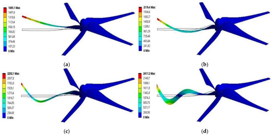

Figure 29.
Modal shapes of blade from first-order to sixth-order: (a) First-order modal shape cloud map of blade; (b) Second-order modal shape cloud map of blade; (c) Third-order modal shape cloud map of blade; (d) Fourth-order modal shape cloud map of blade; (e) Fifth-order modal shape cloud map of blade; (f) Sixth-order modal shape cloud map of blade.
According to the theoretical analysis of blade mode, there are three main modal vibration modes of blade under external frequency excitation: waving vibration, oscillating vibration and torsional vibration. It can be seen from Figure 29 that the first and second-order modal vibration modes of blade are waving vibration. When the external frequency gradually rises to the third-order mode, the blade vibration mode is a mixed vibration dominated by vibration wave and supplemented by oscillating vibration. When the external excitation frequency of the blade continues to increase to the fourth-order mode, the swing of the blade becomes more obvious, which is manifested as the composite vibration of oscillating vibration and waving vibration. With the increase in external frequency, the vibration form of the blade becomes more and more complex, the amplitude becomes larger and larger, and the fifth and sixth vibration modes become more complex, it is no longer a simple combination of two vibration modes, but the coupled vibration of waving, swing and torsion.
In order to further analyze the dynamic performance of the blade under off design conditions, this paper makes the Campbell diagram of the blade according to the above calculation and simulation structure, as shown in Figure 29. In the figure, two horizontal lines represent the first-order natural frequency and the second-order natural frequency, respectively. The vertical line represents the rated speed reached by the wind turbine (224 rad/s). 1P–6P rays represent the integral multiple of the external excitation frequency, respectively. Figure 30 shows that when the external excitation frequency is equal to the natural frequency or integral multiple of the natural frequency of the blade, the blade will resonate. In practice, the external excitation frequency is mostly small, so this paper only studies the modal shapes of the first two frequencies. When the wind turbine speed reaches the rated speed (224 rad/s), the excitation frequency of the blade is 72 Hz, which is far from the first-order natural frequency of the blade of 90.209 Hz, so it is difficult to resonate. The blade is most likely to resonate in the first two orders. However, through the above analysis, it can be found that the wind turbine blade is not easy to resonate in the first two stages, and overall the blade is safe and meets the design requirements. The designed wind turbine blade can provide suggestive guidance for the practical application of mine horizontal axis wind turbine.
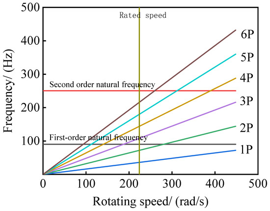
Figure 30.
Campbell diagram of blade.
5. Conclusions
- Based on the blade element momentum and Wilson optimization theory, combined with the MATLAB programming calculation results, the torsional angle and chord length of the wind turbine blade under the optimized conditions are obtained. The data are transformed into three-dimensional model through coordinate transformation.
- Through the static structure analysis of the blade, it can be seen that the overall displacement of the blade is small, and the maximum displacement change occurs at the blade tip. The maximum stress and strain of the blade are located at the root of the blade, and the overall area stress of the blade surface is small. The stress and strain of the blade are lower than the allowable stress and strain of FRP material, so the blade structure is safe. The stress and strain increase with the increase in rotating speed. At low rotating speed, the incoming wind speed plays a leading role, and the change rate of blade displacement, stress and strain is small.
- The first and second modes of the blade are waving vibration. In the third mode, the blade vibration mode is a mixed vibration dominated by vibration wave and supplemented by oscillating vibration. In the fourth mode, the blade vibration mode is a composite vibration of swing and waving vibration, and the main vibration of the blade occurs at the blade tip. In the fifth and sixth modes, the blade vibration mode is a coupled vibration of waving, swing and torsion. The blade vibration occurs in the area between the blade root and the blade. The wind turbine blade is not easy to resonate in the first two steps, and overall the blade is safe.
Author Contributions
Conceptualization, X.G. and H.X.; methodology, X.G.; software, H.X.; validation, X.Z. and F.Z.; formal analysis, X.G.; investigation, X.G.; resources, X.G.; data curation, H.X.; writing—original draft preparation, H.X.; writing—review and editing, X.Z.; visualization, R.G.; supervision, X.G.; project administration, X.G.; funding acquisition, H.X. All authors have read and agreed to the published version of the manuscript.
Funding
This research received no external funding.
Conflicts of Interest
The authors declare that they have no known competing financial interests or personal relationships that could have appeared to influence the work reported in this paper.
References
- Li, X. Explore How to Improve the Safety and Quality Management Level of Coal Mining. Min. Equip. 2021, 11, 166–167. [Google Scholar]
- He, Y.; Liu, W.; Li, Y. On the development of world coal industry. China Coal 2021, 47, 126–135. [Google Scholar]
- Jing, X.; Wang, W.; Hei, L.; Jia, S. Application of wireless sensor network in coal mine safety intelligent monitoring system. Coal Technol. 2009, 28, 93–97. [Google Scholar]
- Qiao, G. Design and Key Technology Research of Coal Mine Safety Integrated Monitoring System Based on Wireless Sensor Network; Lanzhou University of Technology: Lanzhou, China, 2012. [Google Scholar]
- Zhang, J.; Gu, X.; Shi, J. Design of coal mine underground environmental parameter monitoring system based on wireless sensor. Sci. Technol. Innov. 2021, 25, 111–112. [Google Scholar]
- Zheng, W. Application of wireless sensor network in coal mine safety monitoring. Contemp. Chem. Res. 2020, 20, 60–61. [Google Scholar]
- Feng, K. Research on Life Cycle Optimization of Underground Wireless Monitoring System Based on Energy Acquisition; China University of Mining and Technology: Xuzhou, China, 2019. [Google Scholar]
- Feng, K.; Guo, Y.; Zhao, D. Research and design of underground thermoelectric energy collection device. Appl. Electron. Technol. 2018, 44, 93–96. [Google Scholar]
- Tian, L.; Ma, Y. Topology reliability design and optimization analysis of coal mine real-time monitoring based on Internet of things. Met. Mines 2017, 52, 63–66. [Google Scholar]
- Liu, H. Application of wireless sensor network in coal mine safety intelligent monitoring system. Electron. Technol. Softw. Eng. 2020, 9, 9–10. [Google Scholar]
- Zhu, H.; Liang, X.; Shi, Y. On the application of big data in the field of Coal Mine Safety—“Smart mine”. Safety 2018, 39, 13–16. [Google Scholar]
- Huo, Z.; Zhang, Y. 5G communication technology and its application in coal mine. Ind. Min. Autom. 2020, 46, 1–5. [Google Scholar]
- Yadav, D.K.; Mishra, P.; Jayanthu, S.; Das, S.K. On the Application of IOT: Slope Monitoring System for Opencast Mines Based on LoRa Wireless Communication. Arab. J. Sci. Eng. 2021, 1–12. [Google Scholar] [CrossRef]
- Wu, X.; Lee, D. An electromagnetic energy-harvesting device based on high efficiency windmill structure for wireless forest fire monitoring application. Sens. Actuators A Phys. 2014, 219, 73–79. [Google Scholar] [CrossRef]
- Deng, F.; Yue, X.; Fan, X.; Guan, S.; Xu, Y.; Chen, J. Multisource Energy Harvesting System for a Wireless Sensor Network Node in the Field Environment. IEEE Internet Things J. 2019, 6, 918–927. [Google Scholar] [CrossRef]
- Gungor, V.; Hancke, G. Industrial Wireless Sensor Networks: Challenges, Design Principles, and Technical Approaches. IEEE Trans. Ind. Electron. 2009, 56, 4258–4265. [Google Scholar] [CrossRef] [Green Version]
- Sudevalayam, S.; Kulkarni, P. Energy Harvesting Sensor Nodes: Survey and Implications. IEEE Commun. Surv. Tutor. 2011, 13, 443–461. [Google Scholar] [CrossRef] [Green Version]
- Zhang, S.; Chen, L.; Zheng, Y.; Li, Y.; Li, Y.; Zeng, M. How Policies Guide and Promoted Wind Power to Market Transactions in China during the 2010s. Energies 2021, 14, 4096. [Google Scholar] [CrossRef]
- Han, W.; Yang, Z. Four-Dimensional Wind Speed Model for Adequacy Assessment of Power Systems with Wind Farms. IEEE Trans. Power Syst. A Publ. Power Eng. Soc. 2013, 28, 2978–2985. [Google Scholar] [CrossRef]
- Su, Y.; Xie, G.; Xie, F.; Xie, T.; Zhang, Q.; Zhang, H.; Du, H.; Du, X.; Jiang, Y. Segmented wind energy harvester based on contact-electrification and as a self-powered flow rate sensor. Chem. Phys. Lett. 2016, 653, 96–100. [Google Scholar] [CrossRef]
- Zhang, J.H.; Liu, Y.Q.; Tian, D.; Yan, J. Optimal power dispatch in wind farm based on reduced blade damage and generator losses—Science Direct. Renew. Sustain. Energy Rev. 2015, 44, 64–77. [Google Scholar] [CrossRef]
- Pholdee, N.; Bureerat, S.; Nuantong, W. Kriging Surrogate-Based Genetic Algorithm Optimization for Blade Design of a Horizontal Axis Wind Turbine. Comput. Modeling Eng. Sci. 2020, 126, 261–273. [Google Scholar] [CrossRef]
- Debbache, M.; Hazmoune, M.; Derfouf, S.; Ciupageanu, D.A.; Lazaroiu, G. Wind Blade Twist Correction for Enhanced Annual Energy Production of Wind Turbines. Sustainability 2021, 13, 6931. [Google Scholar] [CrossRef]
- Elhenawy, Y.; Fouad, Y.; Marouani, H.; Bassyouni, M. Simulation of Glass Fiber Reinforced Polypropylene Nanocomposites for Small Wind Turbine Blades. Processes 2021, 9, 622. [Google Scholar] [CrossRef]
- Agha, A.; Chaudhry, H.; Wang, F. Diffuser augmented wind turbine (dawt) technologies: A review. Int. J. Renew. Energy Res. 2018, 8, 1369–1385. [Google Scholar]
- Abe, K.; Nishida, M.; Sakurai, A.; Ohya, Y.; Kihara, H.; Wada, E.; Sato, K. Experimental and numerical investigations of flow fields behind a small wind turbine with a flanged diffuser. J. Wind Eng. Ind. Aerodyn. 2005, 93, 951–970. [Google Scholar] [CrossRef]
- Chen, L.; Ponta, F.; Lago, L. Perspectives on innovative concepts in wind-power generation. Energy Sustain. Dev. 2011, 15, 398–410. [Google Scholar] [CrossRef]
- Hendriana, D.; Firmansyah, T.; Setiawan, J.D.; Garinto, D. Design and optimization of low speed horizontal-axis wind turbine-using OpenFOAM. ARPN J. Eng. Appl. Sci. 2015, 10, 21. [Google Scholar]
- Chan, C.; Bai, H.; He, D. Blade shape optimization of the Savonius wind turbine using a genetic algorithm. Appl. Energy 2018, 213, 148–157. [Google Scholar] [CrossRef]
- Özkan, R.; Genç, M. Multi-objective structural optimization of a wind turbine blade using NSGA-II algorithm and FSI. Aircr. Eng. Aerosp. Tech. 2021, 93, 1029–1042. [Google Scholar] [CrossRef]
- Zhu, J.; Cai, X.; Gu, R. Multi-Objective Aerodynamic and Structural Optimization of Horizontal-Axis Wind Turbine Blades. Energies 2017, 10, 101. [Google Scholar] [CrossRef] [Green Version]
- Xin, H.U.A.; Rui, G.U.; Jin, J.F.; Liu, Y.R.; Yi, M.A.; Qian, C.O.N.G.; Zheng, Y. Numerical Simulation and Aerodynamic Performance Comparison between Seagull Aerofoil and NACA 4412 Aerofoil under Low-Reynolds. Adv. Nat. Sci. 2010, 2, 244–250. [Google Scholar]
- Wang, L.; Hu, P.; Lu, J.; Chen, F.; Hua, Q. Neural network and PSO-based structural approximation analysis for blade of wind turbine. Model. Identif. Control 2013, 18, 69–77. [Google Scholar] [CrossRef]
- Xu, L. Research on Mine Ventilation Residual Kinetic Energy Power Generation; Liaoning University of Engineering and Technology: Jinzhou, China, 2012. [Google Scholar]
- Xu, G. Advantages and future development direction of coal mine safety monitoring and upgrading. Chem. Manag. 2020, 33, 90–91. [Google Scholar]
- Jiang, L.; Liu, Y.; Zhao, C. Study on flow field characteristics and calculation of local ventilation resistance coefficient in roadway turning area. Coal Sci. Tech. 2020, 48, 95–102. [Google Scholar]
- Sang, C. Calculation and analysis of wind resistance of wind tunnel based on numerical simulation of wind tunnel flow field. Coal Mine Saf. 2018, 49, 194–199. [Google Scholar]
- Cheng, J. Research on Self-Powered Wireless Sensor Networks Based on Wind Energy Collection; Wuhan University of Technology: Wuhan, China, 2020. [Google Scholar]
- Hansen, M.O.L.; Sørensen, J.N.; Voutsinas, S.; Sørensen, N.; Madsen, H.A. State of the art in wind turbine aerodynamics and aeroelasticity. Prog. Aerosp. Sci. 2006, 42, 285–330. [Google Scholar] [CrossRef]
- Jenkins, P.; Wilsin, A. Analysis of a Diffuser-Augmented, Multi-rotor Wind Turbine System. J. Energy Power Eng. 2018, 13, 419–435. [Google Scholar]
- Gray, A.; Singh, B.; Singh, S. Low wind speed airfoil design for horizontal axis wind turbine. Mater. Today Proc. 2021, 2, 241–250. [Google Scholar] [CrossRef]
- Li, X.; Zhang, L.; Song, J.; Bian, F.; Yang, K. Airfoil design for large horizontal axis wind turbines in low wind speed regions. Renew. Energy 2020, 145, 2345–2357. [Google Scholar] [CrossRef]
- Guo, J. Study on the Mechanism and Control Method of Air Flow Turbulence in the Mine Intake Shaft Region; China University of Mining and Technology (Beijing): Beijing, China, 2016. [Google Scholar]
- Zhu, S.; Xi, F.; Gao, J. Aerodynamic optimization design and three-dimensional modeling of horizontal-axis wind turbine blades. Contemp. Tour. (Golf Travel) 2018, 9, 132+139. [Google Scholar]
Publisher’s Note: MDPI stays neutral with regard to jurisdictional claims in published maps and institutional affiliations. |
© 2021 by the authors. Licensee MDPI, Basel, Switzerland. This article is an open access article distributed under the terms and conditions of the Creative Commons Attribution (CC BY) license (https://creativecommons.org/licenses/by/4.0/).