Article

Optimization-Based Network Identification for Thermal Transient Measurements

1
Faculty of Electrical Engineering, South Westphalia University of Applied Sciences, 59494 Soest, Germany
2
Fraunhofer Application Center for Inorganic Phosphors, Branch Lab of Fraunhofer Institute for Microstructure of Materials IMWS, 59494 Soest, Germany
*
Author to whom correspondence should be addressed.
Energies 2021, 14(22), 7648; https://doi.org/10.3390/en14227648
Submission received: 18 October 2021 / Revised: 11 November 2021 / Accepted: 12 November 2021 / Published: 16 November 2021
(This article belongs to the Special Issue Latest Advances in Electrothermal Models II)

Abstract

:
Network identification by deconvolution is a proven method for determining the thermal structure function of a given device. The method allows to derive the thermal capacitances as well as the resistances of a one-dimensional thermal path from the thermal step response of the device. However, the results of this method are significantly affected by noise in the measured data, which is unavoidable to a certain extent. In this paper, a post-processing procedure for network identification from thermal transient measurements is presented. This so-called optimization-based network identification provides a much more accurate and robust result compared to approaches using Fourier or Bayesian deconvolution in combination with Foster-to-Cauer transformation. The thermal structure function obtained from network identification by deconvolution is improved by repeatedly solving the inverse problem in a multi-dimensional optimization process. The result is a non-diverging thermal structure function, which agrees well with the measured thermal impedance. In addition, the associated time constant spectrum can be calculated very accurately. This work shows the potential of inverse optimization approaches for network identification.

1. Introduction

In thermal response measurements, a system is exposed to a change in heating or cooling power and the response of the system, i.e. the resulting temperature change, is monitored. Typically, the impulse response or the step response is measured with the goal to reconstruct the relevant thermal properties of the system. For the one-dimensional case, this corresponds to the construction of an equivalent Cauer network with known resistances and capacitances. One method to achieve this is known as the “network identification by deconvolution” method [1]. The method is regularly used as an analysis tool for transient thermal analysis [2,3,4]. The methodology itself is also subject to intense discussions [5,6,7,8].
As a first step in this procedure, the measured thermal step response of a device under test, called thermal impedance, is plotted on a logarithmic time scale and differentiated to obtain the logarithmic impulse response. Subsequently, a deconvolution is performed to retrieve the time constant spectrum, which gives the parameters for a Foster-type thermal equivalence network. As the last step, a Foster-to-Cauer transformation is performed to identify the thermal resistances and capacities of the heat path and to construct the thermal structure function.
Network identification by deconvolution is a challenging technique both with respect to measurement setup and evaluation procedure. In their book, Lasance and Poppe state that “ Z th curves must be extremely noise free” ([9], p. 129). An industry standard for the thermal characterization of electronic devices, the JEDEC standard JESD51-14, reports that the solution is “extremely sensitive to noise” ([10], p. 16). Ezzahri and Shakouri note in their paper that the thermal transient should ideally be sampled at least 10 to 15 times faster than the smallest time constant in the signal [11]. A study at Infineon Technologies warns against misinterpretation of numerical artifacts in the structure function, highlighting the importance of accurate algorithms and careful interpretation of the results [12].
The input signal is typically recorded at a constant rate on a linear timescale. The conversion from a linear to a logarithmic scale, z = ln ( t ) , presents a first challenge as it leaves the thermal impedance sparsely sampled in the beginning and dense at the end. The result is a relatively low accuracy for the derivative at short times, which is particularly detrimental for the subsequent, noise sensitive deconvolution. The final step, the Foster-to-Cauer transformation, typically introduces a divergence to the structure function. In principle, the divergence in thermal capacitance reflects the infinite heat capacity of the ambient. In practice, the divergence is significantly smeared out and masks the true behavior of the structure function at the end, which is an artifact of the algorithm [13]. A detailed analysis of the numerical challenges during network identification by deconvolution and suggestions to systematically improve its performance are given in [8].
In this work, an alternative approach is used for the task of network identification. The idea of the so-called optimization-based network identification is to avoid the numerically challenging steps by solving the inverse problem to network identification repeatedly. When solving the equations in this direction, an integration and convolution has to be performed instead of a differentiation and deconvolution. This promises a higher accuracy, as these tasks are numerically much simpler. In optimization-based network identification, an initial estimate for the thermal equivalence network, i.e., the thermal structure function, is first generated by conventional network identification by deconvolution. Next, the solution is refined by a multi-dimensional optimization to find a good match between optimization and measurement data. In this way, the algorithm does not rely on the differentiation and deconvolution of noisy data only.

2. Inverse Calculations

The goal of network identification by deconvolution is to derive a thermal equivalence network, i.e., the thermal structure function, from a thermal transient measurement. In this context, an inverse calculation means to derive a step response from a thermal equivalence network, i.e., a structure function.
The thermal structure function describes a system via numerous small sections with constant resistance and capacitance density, r i and c i . However, real physical systems comprise significantly fewer components. Most of the r i and c i represent the same layer or component. Thus, the relevant information is also captured by a simplified thermal equivalence network, which is constructed from the full thermal structure function. As a model for the simplified thermal network, a chain of uniform RC transmission lines is used [14]. Its corresponding structure function is called piecewise uniform structure function. A comprehensive treatment of non-uniform RC lines can be found in [15,16]. Once the total resistances, R i , and the total capacitances, C i , of each section of the piecewise uniform transmission line are known, its total impedance can be constructed. The impedance up to each section, Z i ( s ) , can be calculated via
Z i ( s ) = R i s C i Z L , i + R i s C i tanh ( s R i C i ) R i s C i + Z L , i tanh ( s R i C i ) .
Here, Z L , i denotes the load impedance of section i and s the complex frequency. The total impedance of the entire transmission line, Z ( s ) , is calculated sequentially by using the input impedance of the previous section as the load impedance of the next. The calculation begins at the short-circuited end with a vanishing load impedance. In 
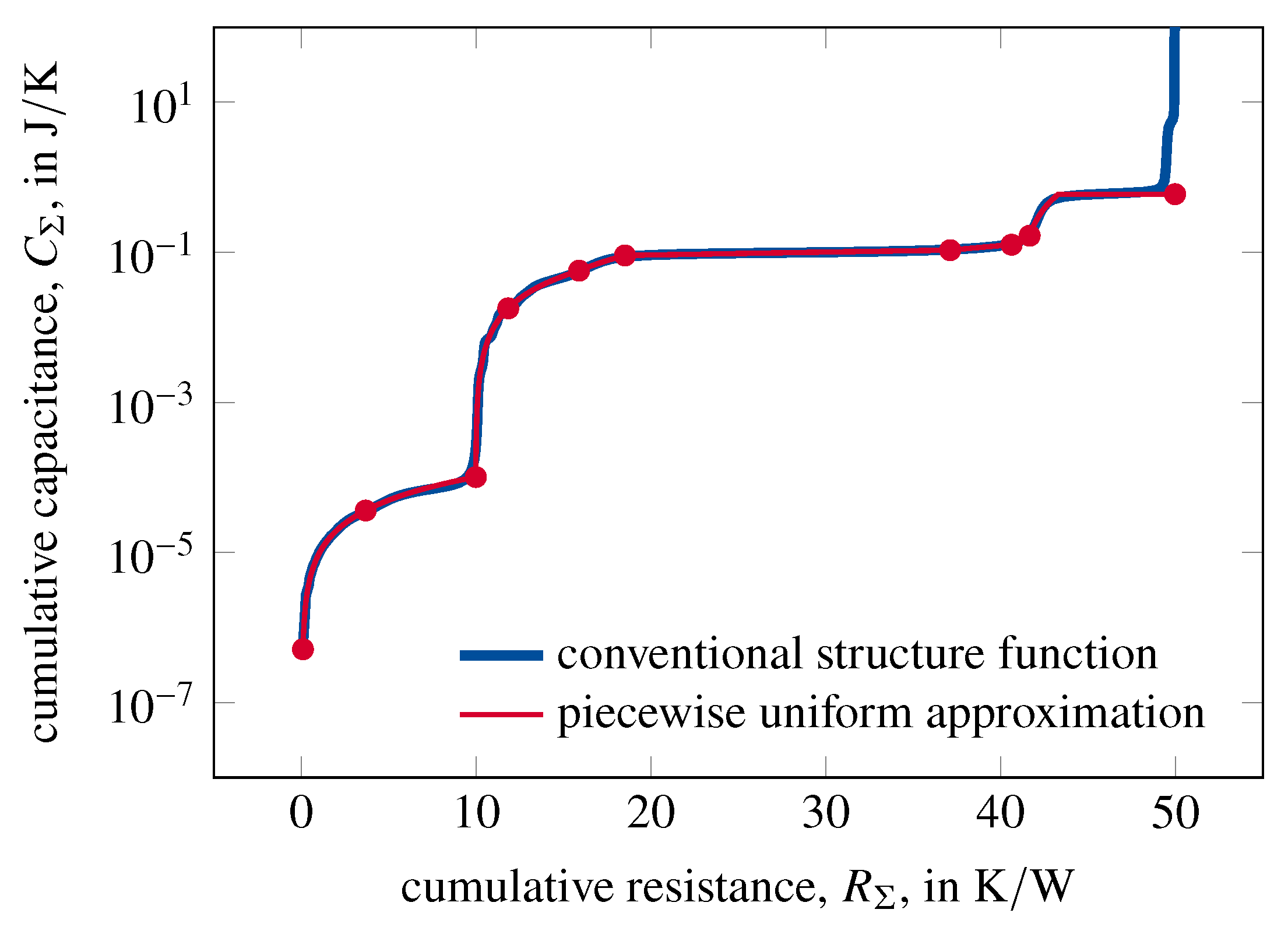
Figure 1, a structure function calculated via network identification by deconvolution is shown together with a piecewise uniform approximation comprising ten sections. Note that due to the decadic logarithmic scaling of the cumulative capacitance the sections do not appear linear.
Once Z ( s ) is known, the logarithmic time constant spectrum, R ( ζ ) , is calculated. It is proportional to the imaginary part, , of Z ( s ) on a path along the negative real axis,
R ( ζ ) = 1 π [ Z ( s = exp ( ζ ) ) ] .
Due to poles on this path, Equation (2) cannot be evaluated directly. Instead, a small angle, δ , is introduced which rotates the path into the complex plane,
s = ( cos ( δ ) + i sin ( δ ) ) exp ( ζ ) .
This has the effect of smoothing the poles, making them finite as described in [17]. The smaller δ is, the more accurate the calculations become. However, a small angle of δ produces high and narrow peaks, which requires a dense sampling of s to be captured correctly. Moreover, for accurate calculations it is required to capture all side lobes of the time constant spectrum. This means, that for small angles of δ the time constant spectrum has to be sampled densely over a wide range. In effect, calculating theoretical thermal impedances with very high accuracy becomes computationally demanding, requiring calculation times of up to several minutes on an ordinary desktop computer. In the literature, it is stated that the angle, δ , should not exceed 5 ° [17]. Typically, the time constant spectrum is sampled at approximately 30 points per decade [18,19].
Ideally, the asymptotic value of the thermal impedance, Z th ( t ) , should match the total thermal resistance of the structure function, R th , Σ , exactly. In this case, the relation R th , Σ = Z th ( t ) is exactly satisfied. However, due to the discretization error and the finite angle, δ , the asymptotic thermal impedance, Z th ( t ) , is different from R th , Σ . The absolute difference between them is denoted as Δ R th , i.e., Δ R th = | R th , Σ Z th ( t ) | .
In the following, an analysis is performed to determine appropriate parameters for inverse calculations. The accuracy is mainly determined by the angle δ and the sampling parameters. The computational workload depends significantly on the number of points used for ζ . To strike a balance between computation time and accuracy, 10 6 points in the range [ 20 , 10 ] are used. To determine an optimum value of δ for this sampling rate, a test series is performed. 
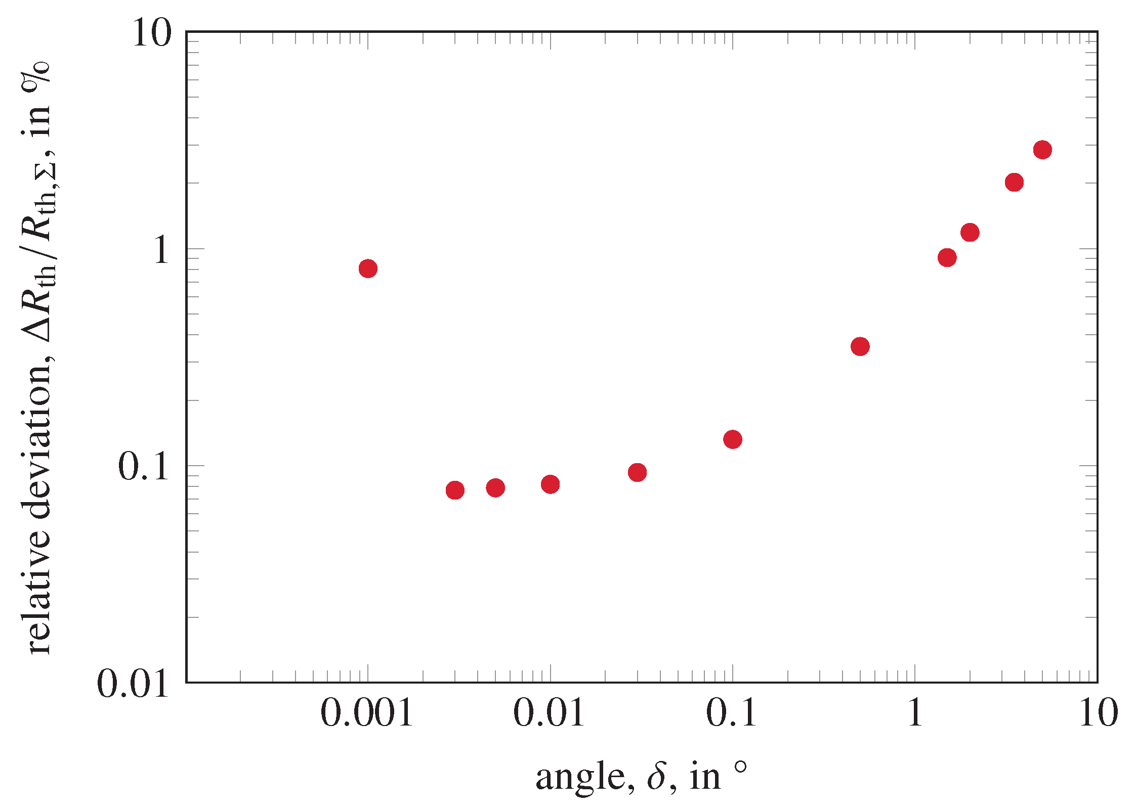
Figure 2 shows the relative deviation, Δ R th / R th , Σ for different values of δ and fixed sampling frequency. As a test case, structure 1 (see Table 1) is used. At high angles, the accuracy is relatively low due to the error made in Equation (3). At very low angles of δ , the peaks are too narrow to be captured correctly, given the sampling frequency. A value of δ = 0.03 ° limits the error made in Equation (3) while making sure that all peaks are captured correctly. For smaller angles and higher sampling frequencies, the error is also limited by the width of the chosen interval.

3. Optimization-Based Network Identification

The idea of optimization-based network identification is to find a piecewise uniform structure function via multi-dimensional optimization, which has a thermal impedance which matches well with the measured thermal impedance. In this way, a structure function belonging to the system is known by definition and the associated time constant spectrum can be readily calculated with high accuracy.
The scheme of Figure 3 visualizes the procedure of optimization-based network identification. Starting from the measured step response (top left), a conventional network identification by deconvolution is performed first. Then, a network simplification is performed (see Figure 1). In this step, the thermal structure function resulting from network identification by deconvolution is approximated by a piecewise uniform structure function, truncating the divergence at the end. A multi-dimensional optimization is performed, which optimizes the resistance and capacitance of each section. The goal is to minimize the discrepancy between the conventional thermal network and the simplified thermal network with a given number of sections. As a last step, an optimization-based network identification is performed. In this step, the simplified thermal network is optimized to best match the measured thermal impedance. The result is the optimized thermal network. For each function evaluation during the optimization, an inverse calculation is performed. Once the optimized thermal network is in good agreement with the measured thermal impedance, the optimization is successful.
For the success of optimization-based network identification, it is important to have good initial values. A strategy to obtain good initial values is to perform a conventional network identification by deconvolution first. To ensure a good fit between the intermediate thermal network, C Σ , intermediate ( R Σ ) , and the thermal structure function, C Σ ( R Σ ) , an optimization is performed during network simplification. The number of piecewise uniform sections, N S , in the step of network simplification is chosen manually. Typically, a suitable number of sections lies between 2 and 20. The number of sections has to be high enough to provide a sufficient number of degrees of freedom while keeping the optimization as simple as possible. Each section is completely defined by the thermal resistance and the thermal capacitance it contributes to the structure function. For the optimization, the best-performing objective function is the square root of the integral of the squared logarithmic deviations, i.e.,
o struc = 0 R log ( C Σ , intermediate ( R Σ ) ) log ( C Σ ( R Σ ) ) 2 d R Σ .
The initial intermediate thermal network, i.e., the starting values for the optimization during the network simplification, are given by points, ( R Σ , i , C Σ , i ) , evenly spaced along the arc length of the forward structure function. In addition, truncating the divergence at high R Σ , which is a numerical artifact of the Foster-to-Cauer transformation, increases the accuracy and the stability of the convergence. For a good convergence, it should be ensured that the total thermal resistance of the initial intermediate thermal network is identical to the total thermal resistance of the measured thermal impedance.
The degrees of freedom provided to the solver are the cumulative resistances and the cumulative capcitances, ( R Σ , 1 , , R Σ , N S , C Σ , 1 , , C Σ , N S ) , of the piecewise uniform structure function. In this way, the total thermal resistance represented by the piecewise uniform structure function is only determined by R Σ , N S and does not change when modifying the other R Σ , i .
The objective function employed for the main optimization is given in (5). It has the form of an L 2 -norm, i.e., it is the square root of the integral of the squared difference between optimized and measured step response,
o imp = z min z max a measured ( z ) a opt ( z ) 2 d z .
Note that a measured ( z ) is typically not evenly spaced. The optimized thermal impedance, a opt ( z ) , is interpolated to be defined on the same set of z i as the measurement data.
To compare the optimized thermal impedance to results from a network identification by deconvolution, the time constant spectrum, which appears during network identification by deconvolution, is reconvolved. Subsequently, it is integrated to reproduce a thermal impedance. This impedance is henceforth called backwards thermal impedance. It is the impedance represented by the time constant spectrum, i.e., it reflects the effects of differentiation and deconvolution. To have a valid solution, the discrepancy (as measured by o imp ) between the optimized thermal impedance and the measured thermal impedance must be similar or even smaller than the discrepancy between the optimized thermal impedance and the backwards thermal impedance.
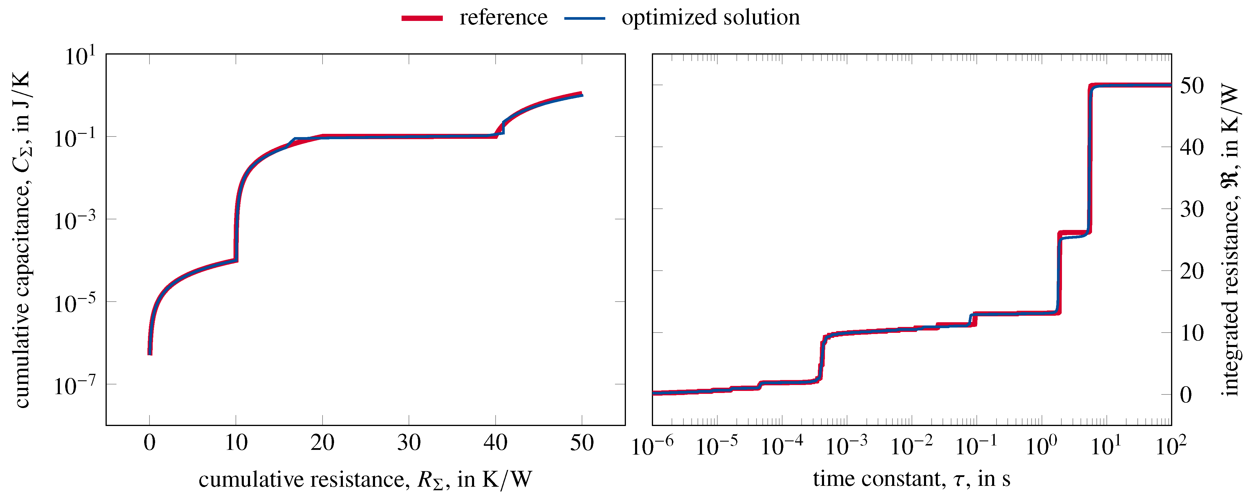
For network simplification as shown exemplarily in Figure 1, the results of the following optimization-based network identification are shown in Figure 4. The value of the objective function resulting from the initial simplified thermal network is o imp , initial   =   1.1449 . After the main optimization, the value of the objective function is reduced to o imp , optimized   =   0.0305 . For comparison, the value of the objective function for the backwards thermal impedance is o imp , backwards   =   0.0244 . To calculate accurate structure functions, a low value of o imp is an important sanity check and suitable to validate solutions. However, it is not a sufficient measure of accuracy for a solution. A holistic comparison of the accuracy of various methods is performed in the following section.
For optimization of the objective function (5), two solvers yield good results. Powell’s conjugate direction method provides a good convergence [20], while constrained Optimization BY Linear Approximations, abbreviated COBYLA, is also suitable [21]. A common feature of both solvers is that they do not calculate derivatives of the objective function and are therefore suitable for problems with complicated objective functions.
Moreover, both solvers are able to respect boundary conditions which is used here to restrict the search space to physically possible values. For example, it is required that all cumulative resistances and capacitances are positive. Additionally, the total thermal resistance, R Σ , N S , is unlikely to significantly exceed Z th ( t ) .
As a physical constraint, the structure function must be monotonically increasing. This means that both the list of resistances, ( R Σ , 1 , , R Σ , N S ) , and capacitances, ( C Σ , 1 , , C Σ , N S ) , should be strictly monotonically increasing, i.e., each R Σ , i and C Σ , i has to be greater than its left neighbor and smaller than its right neighbor. However, the solvers do not uphold these conditions during the optimization strictly. There has to be a mechanism to repair unphysical structure functions that appear during the optimization. This is done by sorting the R Σ , i and C Σ , i in each evaluation. Furthermore, a minimum size for R Σ , i R Σ , i + 1 and C Σ , i C Σ , i + 1 is set to avoid numerical instability.
In general, the COBYLA solver is able to accept constraints, that force the parameters to fulfill certain boundary conditions. This can be used to restrict the solution to remain physically meaningful in the sense explained above. Still, validity should be checked every function evaluation because of possible constraint violations. Furthermore, significant speed increases for the Powell solver are achieved by using an LRU (least recently used) cache on parts of Equation (1). On the computer used in this work (Windows 10, Intel Core i7-8665U CPU with 1.90 GHz, 16 GB RAM), the computation time for an optimization-based network identification is on the order of a few minutes depending on the speed of convergence for the specific problem. The conventional network identification by deconvolution, which is performed at first, takes a few seconds.

4. Methodology

Three reference structures are defined to compare the performance of optimization-based network identification with that of other methods such as network identification using Fourier or Bayesian deconvolution (Table 1). To judge the accuracy of each method, the exact thermal impedance of each reference structure is calculated as described in Section 2. This thermal impedance is then used as input data for a network identification algorithm. The accuracy of each method is measured by comparing the recovered structure functions and time constant spectra with the reference.
To evaluate the algorithms under different conditions, the sampling rate and the signal-to-noise ratio of the reference thermal impedances are artificially degraded. As a first test case, the exact thermal impedance is provided to the algorithm without noise and with a high sampling rate. This allows to judge the performance of the algorithms for perfect input data. Second, an imperfect measurement is simulated by a reduction of the sampling rate and the addition of Gaussian noise. The corresponding standard deviation, σ , is defined by the signal-to-noise ratio, R SN , and the asymptotic thermal impedance, Z th ( t ) , via
R SN = Z th ( t ) σ .
Third, in addition to the introduction of noise, the thermal impedance is resampled with a constant sampling rate in linear time, t. This results in unevenly spaced points in logarithmic time, z.
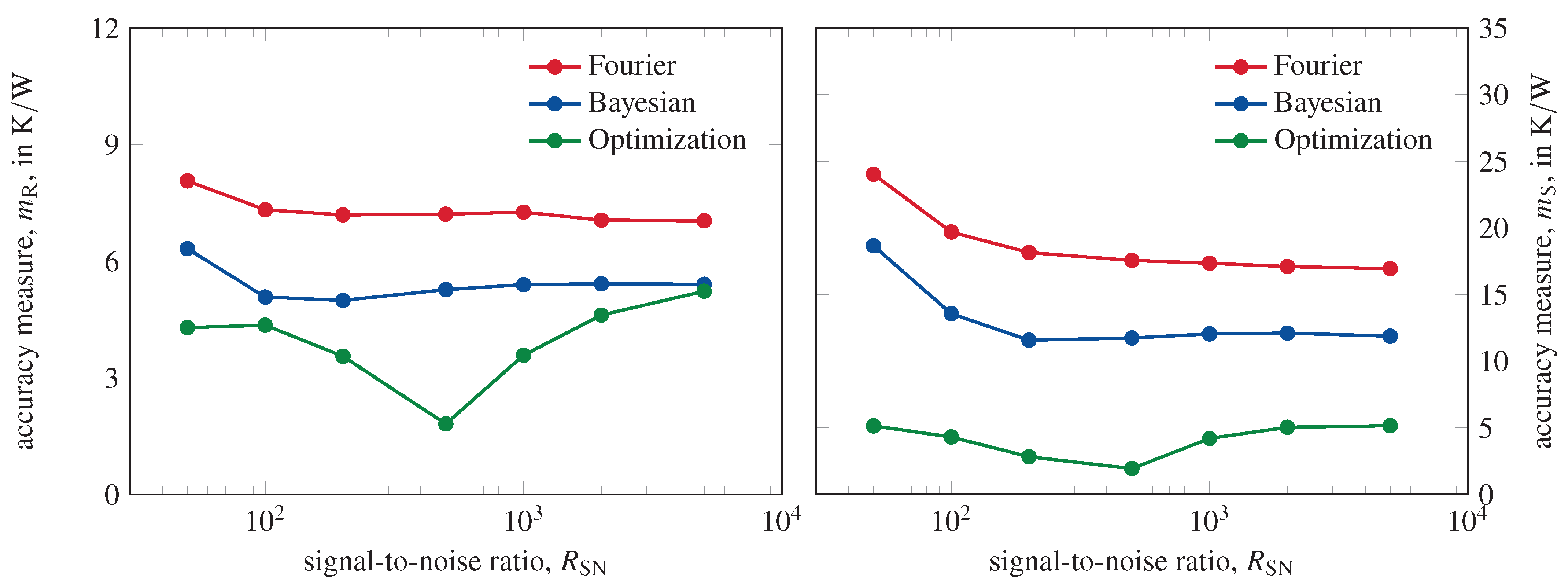
For the comparison of the recovered solutions with the theoretically ideal reference, several measures of accuracy are defined. For a derivation and discussion of these measures of accuracy, the reader is referred to ([8] Section 3.1—Measures of Accuracy). There, also an analysis of network identification algorithms using Fourier and Bayesian deconvolution on the basis of these measures is given (Section 6—Performance Quantification). The calculations presented here are conducted as similarly as possible to allow a fair comparison.
To quantify differences between two time constant spectra, the integrated spectrum, R ( ζ ) , is used, i.e.,
R ( ζ ) = ζ R ( ζ ) d ζ .
The measure of accuracy for time constant spectra, m R , is then defined as an L 2 -norm of the differences between the integrated spectra,
m R = R theo ( ζ ) R ( ζ ) 2 d ζ .
When comparing two structure functions, a suitable definition for the integration limits is crucial, as there are divergences in the structure function and potentially different domains. The lower integration limit, R Σ , min , and the upper integration limit, R Σ , max , are defined as
R Σ , max = arg max ( C Σ ) and R Σ , min = arg min ( C Σ , theo )
where C Σ , theo is the theoretical reference structure function and C Σ is the structure function it is compared to. Using these definitions, the measure of accuracy for structure functions, m S , is
m S = R Σ , min R Σ , max | log ( C Σ , theo ( R Σ ) ) log ( C Σ ( R Σ ) ) | d R Σ .
Here, C Σ ( R Σ ) is measured in units of J / K . To assess the absolute accuracy of the total thermal resistance, a third measure of accuracy, Δ R Σ , is required [8], as the upper integration limit, R Σ , max , is defined by the recovered structure function itself,
Δ R Σ = | R Σ , th R Σ , max | .
Here, R Σ , th is the exact thermal resistance.

5. Performance

5.1. Performance for the Case of Perfect Data

First, the performance of optimization-based network identification is analyzed in the ideal case of noise-free measurement data. A test of the algorithm on experimental data is presented in [7]. The exact thermal impedance provided as input consists of 10 6 points for ζ uniformly distributed in the range [ 20 , 10 ] . A summary of the results is given in Table 2. To allow a fair comparison between the different methods under study, all parameters are chosen to be identical for all methods and structures wherever possible. In particular, this includes the network identification by deconvolution, which is computed as part of the optimization-based network identification, which uses a Bayesian deconvolution. The accuracies for the Fourier and Bayesian methods in Table 2 are taken from [8]. For the case of Fourier domain deconvolution, the Hann filter is chosen.
For optimization-based network identification, several parameters have to be specified. This includes termination and convergence criteria for the iteration such as the maximum number of iterations, the acceptable relative error in ( R Σ , 1 , , R Σ , N S , C Σ , 1 , , C Σ , N S ) , and the acceptable relative error in the objective function, o imp , as defined in Equation (5). For the use of a COBYLA solver, a tolerance for constraint violations must be set. A robust configuration is found for these parameters, which will be used in the following.
The accuracy also depends on the number of uniform sections used in the step of network simplification. For this parameter, the optimum value is used for each test structure. As many inverse calculations are required to perform an optimization-based network identification, each thermal impedance is calculated with reduced accuracy compared to the input data. Here, an angle of δ = 0.5 ° with 104 points for ζ [ 20 , 10 ] is used.
The results presented in Table 2 show the method with the best performance for each accuracy measure and structure in bold, the second-best result is underlined. In terms of m S and m R , the optimization-based network identification with a Powell solver performs best for all test structures, while the second-best result is consistently obtained by optimization-based network identification with a COBYLA solver. The best resistance accuracy, Δ R Σ , is achieved in all cases by network identification via Bayesian deconvolution. This comes from the property of Bayesian deconvolution to preserve the total resistance during deconvolution.

5.2. Performance in the Presence of Noise

Next, the performance of optimization-based network identification when confronted with noisy input data is evaluated. A summary of the accuracy values for test structure 1 is given in Table 3. Tests on structures 2 and 3 reveal similar trends.
As input data, the exact thermal impedance is interpolated to 1000 uniformly distributed points for ζ [ 20 , 10 ] . To each data point Gaussian noise is added according to (6). The tested signal-to-noise ratios are 50, 100, 200, 500, 1000, 2000, and 5000. To provide an example, a signal-to-noise ratio of R SN = 5000 corresponds to a transient thermal measurement with a total temperature rise of 100 K , which is observed with an accuracy of 20 m K .
As the results should not depend on a single distribution of noise only, 2000 independent realizations of noise are randomly generated. Each method is tested with the same set of randomly generated measurement data. As a result, the median over the recovered structure functions and the recovered integrated time constant spectra are calculated. For this, the structure functions are interpolated to a common set of R Σ , i . Subsequently, the median functions are inserted into the measures of accuracy Equations (8), (10), and (11). Results comparing the performance of Fourier deconvolution, Bayesian deconvolution, and optimization-based network identification are presented in Table 3. The computations employing Fourier and Bayesian deconvolution are conducted exactly as described in [8].
For optimization-based network identification, the number of sections in the piecewise uniform approximation is set to six. While this does not necessarily provide the best accuracy possible, a low number of sections reduces the computation time significantly. The total computation time for 2000 optimization-based network identifications, when calculated in series, is on the order of days. The precise computation time of an optimization-based network identification depends on the trajectory the solver takes in parameter space, which is mainly affected by the quality of the initial values and the noise level.
Table 3 shows that for both m R and m S the optimization-based network identification performs best and the Fourier deconvolution performs worst for all signal-to-noise ratios. In particular for high noise levels, optimization-based network identification achieves a significant improvement in accuracy. In addition, the accuracy of optimization-based network identification is much less affected by lower signal-to-noise levels.

5.3. Constant Frequency Sampling with Noise

In a last step, the quality of the data is reduced further. The exact thermal impedance is resampled using a fixed sampling rate in linear time of 107 and also including the starting point of the original impedance at t = 2 × 10 9 . To limit the number of data points, the sampling rate is slowed down beyond a certain density of points in logarithmic time, z, which is constant from there on. The total number of data points for constant frequency sampling amounts to 784.
An example of a thermal impedance with a signal-to-noise-ratio of R SN = 50 is shown on the bottom right of Figure 5. In addition, the backwards thermal impedance from Bayesian deconvolution and the optimization-based solution are plotted. The other parts of the image show the corresponding evaluations using Bayesian deconvolution and optimization-based network identification. The impulse response and thermal impedance for the Bayesian solution are generated by reconvolving the time constant spectrum. This is done to reveal effect of deconvolution and to shown the impulse response as well as the thermal impedance actually belonging to the time constant spectrum. The exact input data belonging to structure 1 are shown for comparison.
In Table 4, the accuracy values achieved by the Bayesian and the optimized solution are shown in addition to the median accuracy values, which are taken from Figure 6. The noise pattern presented in Figure 5 leads to a solution with a quality significantly below average. Still, the optimization algorithm is able to increase the accuracy of the time constant spectrum and the structure function. The thermal impedance resulting from an optimization-based network identification matches better with the exact thermal impedance of structure 1 than the original Bayesian solution. While the optimization procedure is able to increase the accuracy of a forward solution significantly, it is still based on the initial values. The optimization might converge to a local minimum which does not represent the global optimum.
For a systematic analysis of the performance, 2000 sets of the resampled noisy thermal impedances are generated and their respective solutions are averaged by calculating the median. Each of the 2000 Bayesian solutions is used to generate the initial values for the corresponding optimization. In the case of Fourier deconvolution, the filter width of the Hann filter employed is fine-tuned for each noise level.
As expected, the Fourier deconvolution still performs the worst on all metrics. The Bayesian solution is improved by the optimization-based network identification for all noise levels. Concerning the optimization-based network identification, the accuracy of the structure function is only marginally affected by the constant frequency sampling.
As solvers for the optimization-based network identification, the Powell solver is faster than COBYLA, but less reliable as sometimes it fails to converge. COBYLA is slower but more stable due to more stringent constraints. On average, the accuracy is similar for both solvers, possibly slightly better for the Powell solver. The non-monotonic behavior of the optimization results in Figure 6 is attributed to a decreased quality of the Bayesian initial values in the case of constant frequency sampling. This forces the solver to take a longer path in parameter space, leading to a larger spread of the results. Fine-tuning the differentiation parameters to each noise level would further improve the average quality of the initial values leading to more reliable convergences.

6. Conclusions

In this work, an alternative evaluation method is presented to generate thermal structure functions from transient thermal measurements. The presented optimization-based method is able to reliably improve the accuracy of a previous solution by solving the inverse network identification problem repeatedly.
To quantify the performance of the optimization-based network identification and to compare it with other methods, three measures of accuracy and three test cases are set up. Tests on noisy and noise-free data show a significant improvement in accuracy in the time constant spectra and the structure functions. In particular for low signal-to-noise ratios, bypassing the process of differentiation and deconvolution provides a clear advantage over conventional network identification. The first test case with perfect data shows that optimization-based network identification using Powell (COBYLA) solvers achieve an average performance advantage in terms of m R and m S by a factor of 2.5 (1.9) compared to Bayesian deconvolution and 4.7 (3.6) compared to Fourier deconvolution. The second test case with added noise reveals that Bayesian deconvolution slowly loses its accuracy advantage over Fourier deconvolution with increasing noise levels. The test of constant frequency sampling with noise shows that there is further potential to refine the optimization routine and to increase the performance advantage. Future goals are to improve the speed and the convergence reliability even further, in particular for inaccurate initial values.
When working with experimental data, optimization-based network identification opens up new possibilities for the evaluation. As the optimization is based on a physical model to generate the thermal impedances, it is not necessary to perform an extrapolation to hide the electrical transient. An extrapolation for low times is naturally generated by the algorithm. The division of the thermal structure function into sections given by the algorithm can help to interpret the structure function and to attribute its shape to the components of the device under test. Moreover, the interpretation is not complicated by a divergence, which is a purely numerical artifact.

7. Patents

The technical content of the paper is related to a patent held by the authors under DE 10 2019 214 472.

Author Contributions

N.J.Z.: Conceptualization, methodology, software, investigation, writing—original draft preparation; P.W.N.: Conceptualization, validation, writing—review and editing; S.S.: Supervision, writing—review and editing. All authors have read and agreed to the published version of the manuscript.

Funding

This publication is funded by the Open Access Publication Fund of South Westphalia University of Applied Sciences.

Conflicts of Interest

The authors declare no conflict of interest.

References

  1. Van Bien, V.S.T. Fine structure of heat flow path in semiconductor devices: A measurement and identification method. Solid-State Electron. 1988, 31, 1363–1368. [Google Scholar] [CrossRef]
  2. Farkas, G.; Poppe, A.; Gaal, L.; Hantos, G.; Bornoff, R.; Rencz, M. Assessment of the validity of multi-domain LED model parameters in a broad current and temperature range. In Proceedings of the 2019 25th International Workshop on Thermal Investigations of ICs and Systems (THERMINIC), Lecco, Italy, 25–27 September 2019; pp. 1–8. [Google Scholar] [CrossRef]
  3. Mitterhuber, L.; Magnien, J.; Siroky, G.; Kieslinger, D.; Kraker, E. TSEP-Sensitivity Study to Analyze the Soldering Process of a Power Diode. In Proceedings of the 2020 26th International Workshop on Thermal Investigations of ICs and Systems (THERMINIC), Berlin, Germany, 24 September 2020; pp. 1–6. [Google Scholar] [CrossRef]
  4. Szőke, S.; Kórádi, Z. Component Model Calibration Using Transient Thermal Test Methods and Multiple Measurement Setups. In Proceedings of the 2019 25th International Workshop on Thermal Investigations of ICs and Systems (THERMINIC), Lecco, Italy, 25–27 September 2019; pp. 1–5. [Google Scholar] [CrossRef]
  5. Pareek, K.A.; Grosse, C.; Sternberg, M.; May, D.; Ras, M.A.; Wunderle, B. Effect of Different Deconvolution Methods on Structure Function Calculation. In Proceedings of the 2020 26th International Workshop on Thermal Investigations of ICs and Systems (THERMINIC), Berlin, Germany, 24 September 2020; pp. 97–104. [Google Scholar] [CrossRef]
  6. Poppe, A.; Vass-Varnai, A.; Sarkany, Z.; Rencz, M.; Hantos, G.; Farkas, G. Suggestions for extending the scope of the transient dual interface method. In Proceedings of the 27th International Workshop on Thermal Investigations of ICs and Systems (THERMINIC), Berlin, Germany, 23 September 2021; pp. 23–30. [Google Scholar]
  7. Ziegeler, N.J.; Nolte, P.W.; Schweizer, S. Optimization-based network identification for thermal transient measurements on LEDs. In Proceedings of the 27th International Workshop on Thermal Investigations of ICs and Systems (THERMINIC), Berlin, Germany, 23 September 2021; pp. 23–30. [Google Scholar]
  8. Ziegeler, N.J.; Nolte, P.W.; Schweizer, S. Quantitative Performance Comparison of Thermal Structure Function Computations. Energies 2021, 14, 7068. [Google Scholar] [CrossRef]
  9. Lasance, C.J.M.; Poppe, A. Thermal Management for LED Applications; Solid State Lighting Technology and Application Series; Springer: New York, NY, USA, 2016. [Google Scholar]
  10. JC-15. Transient Dual Interface Test Method for the Measurement of the Thermal Resistance Junction to Case of Semiconductor Devices with Heat Flow Trough a Single Path; Standard JESD51-14; JEDEC Solid State Technology Association: Arlington, TX, USA, 2010. [Google Scholar]
  11. Ezzahri, Y.; Shakouri, A. Application of network identification by deconvolution method to the thermal analysis of the pump-probe transient thermoreflectance signal. Rev. Sci. Instrum. 2009, 80, 074903. [Google Scholar] [CrossRef] [PubMed]
  12. Schweitzer, D.; Pape, H.; Chen, L. Transient measurement of the junction-to-case thermal resistance using structure functions: Chances and limits. In Proceedings of the Twenty-fourth Annual IEEE Semiconductor Thermal Measurement and Management Symposium, San Jose, CA, USA, 16–20 March 2008; pp. 191–197. [Google Scholar] [CrossRef]
  13. Salleras, M.; Palacin, J.; Carles, G.; Marco, S. Difficulties on the estimation of the thermal structure function from noisy thermal impedance transients. In Proceedings of the International Conference on Thermal and Mechanical Simulation and Experiments in Microelectronics and Micro-Systems, Como, Italy, 24–26 April 2006; pp. 1–7. [Google Scholar] [CrossRef]
  14. Chen, W.K. Feedback, nonlinear, and distributed circuits. In The Circuits and Filters Handbook, 3rd ed.; Chapter Distributed RC Networks; CRC Press: Boca Raton, FL, USA, 2009. [Google Scholar]
  15. Protonotarios, E.N.; Wing, O. Theory of nonuniform RC lines, part I: Analytic properties and realizability conditions in the frequency domain. IEEE Trans. Circuit Theory 1967, 14, 2–12. [Google Scholar] [CrossRef]
  16. Protonotarios, E.N.; Wing, O. Theory of nonuniform RC lines, part II: Analytic properties in the time domain. IEEE Trans. Circuit Theory 1967, 14, 13–20. [Google Scholar] [CrossRef]
  17. Vladimir, S.A.S. Possible acception criteria for structure functions. Microelectron. J. 2012, 43, 164–168. [Google Scholar] [CrossRef]
  18. Székely, V. Evaluation of short pulse thermal transient measurements. In Proceedings of the 14th International Workshop on Thermal Inveatigation of ICs and Systems, Rome, Italy, 24–26 September 2008; pp. 20–25. [Google Scholar] [CrossRef]
  19. Székely, V.; Rencz, M. Thermal dynamics and the time constant domain. IEEE Trans. Compon. Packag. Technol. 2000, 23, 587–594. [Google Scholar] [CrossRef]
  20. Powell, M.J.D. An efficient method for finding the minimum of a function of several variables without calculating derivatives. Comput. J. 1964, 7, 155–162. [Google Scholar] [CrossRef]
  21. Powell, M.J.D.; Hennart, J.P. A direct search optimization method that models the objective and constraint functions by linear interpolation. In Advances in Optimization and Numerical Analysis; Springer: Dordrecht, The Netherlands, 1994; pp. 51–67. [Google Scholar] [CrossRef]
Figure 1. Conventional structure function and piecewise uniform approximation with ten sections. The divergence at the end is truncated in the optimization as it is a numerical artifact.
Energies 14 07648 g001
Figure 2. Relative deviation in thermal resistance for structure 1 at 10 6 points for ζ [ 20 , 10 ] .
Energies 14 07648 g002
Figure 3. Scheme for optimization-based network identification. First, a network identification by deconvolution is performed. Then, the steps of network simplification and optimization-based network identification follow.
Energies 14 07648 g003
Figure 4. Result for the optimization-based network identification using the Powell solver with ten sections. The initial values are as shown in Figure 1. The measures of accuracy are m R = 3.52 and m S = 2.46 . For the calculation, structure 2 is used as an example (see Table 1).
Energies 14 07648 g004
Figure 5. Example solution for network identification using Bayesian deconvolution and Powell optimization on the basis of six sections for a single realization of sparse noisy data with R SN = 50 . The Bayesian solution is used to generate initial values for the optimization. In Table 4 the corresponding accuracy values are summarized.
Energies 14 07648 g005
Figure 6. Accuracy of the median integrated time constant spectrum and median structure function for Fourier deconvolution, using a Hann filter, Bayesian deconvolution and the optimization-based network identification using the Powell solver, calculated from 2000 noise realizations for structure 1.
Energies 14 07648 g006
Table 1. For the purpose of comparison, three reference structures are defined as a chain of uniform RC transmission lines, where each section has a thermal resistance and capacitance.
Structure 1Structure 2Structure 3
R th C th R th C th R th C th
Sections K / W J/K K / W J/K K / W J/K
Section 1510−51010−42010−1
Section 21510−31010−12010−4
Section 31010−41010−41010−3
Section 41010−21010−3--
Section 51010−110100--
Table 2. Best accuracy for all methods in the absence of noise. The best performing method in each column is highlighted in bold, the second best result is underlined.
MethodStructure 1Structure 2Structure 3
m R m S Δ R Σ m R m S Δ R Σ m R m S Δ R Σ
K / W K / W K / W K / W K / W K / W K / W K / W K / W
Fourier4.47.40.286.37.50.448.910.80.91
Bayesian3.43.70.043.84.40.025.73.10.01
Powell1.21.20.132.01.30.142.41.80.15
COBYLA1.52.00.132.42.60.142.51.90.14
Table 3. Accuracy for all methods as a function of the signal-to-noise ratio, R SN .
R SN FourierBayesianPowell
m R m S m R m S m R m S
K / W K / W K / W K / W K / W K / W
508.8124.47.5923.04.145.6
1007.1318.05.2713.43.793.8
2006.6214.34.398.83.492.6
5006.2211.64.076.03.152.1
10005.8710.54.005.02.922.0
20005.849.93.984.52.842.0
50005.669.03.984.22.662.0
Table 4. Accuracy values for the solutions in Figure 5 and comparisons to the respective median values from Figure 6.
BayesianPowellBayesian MedianPowell Median
m R in K / W 9.804.686.324.29
m S in K / W 27.097.2518.665.14
Publisher’s Note: MDPI stays neutral with regard to jurisdictional claims in published maps and institutional affiliations.

