Article

Empirical Validation of a Biogas Plant Simulation Model and Analysis of Biogas Upgrading Potentials †

by
Jan Martin Zepter
,
Jan Engelhardt
,
Tatiana Gabderakhmanova
and
Mattia Marinelli
*
Center for Electric Power and Energy, Department of Electrical Engineering, Technical University of Denmark (DTU), Risø Campus, 4000 Roskilde, Denmark
*
Author to whom correspondence should be addressed.
This paper is an extended version of our paper published in the Proceedings of the 2020 55th International Universities Power Engineering Conference (UPEC), Turin, Italy, 1–4 September 2020.
Energies 2021, 14(9), 2424; https://doi.org/10.3390/en14092424
Submission received: 26 March 2021 / Revised: 16 April 2021 / Accepted: 17 April 2021 / Published: 24 April 2021

Abstract

:
Biogas plants may support the transformation towards renewable-based and integrated energy systems by providing dispatchable co-generation as well as opportunities for biogas upgrading or power-to-X conversion. In this paper, a simulation model that comprises the main dynamics of the internal processes of a biogas plant is developed. Based on first-order kinetics of the anaerobic digestion process, the biogas production of an input feeding schedule of raw material can be estimated. The output of the plant in terms of electrical and thermal energy is validated against empirical data from a 3-MW biogas plant on the Danish island of Bornholm. The results show that the model provides an accurate representation of the processes within a biogas plant. The paper further provides insights on the functioning of the biogas plant on Bornholm as well as discusses upgrading potentials of biogas to biomethane at the plant from an energy perspective.

1. Introduction

In future power systems, the high shares of renewable energy sources such as wind and solar photovoltaics (PV) challenge grid operations with intermittent and non-dispatchable electricity generation. The power injections of these sources into the grid are only partly controllable as their generation depends on local weather conditions. In addition, they do not supply the system with extensive flexibility to align the generation with the consumption side, making real-time matching more difficult. Together with hydropower plants as well as (battery) storage systems, biogas plants running on organic waste depict one central element of reliable future low-carbon multi-energy systems. In their structure as co-generation units, biogas plants contribute significantly to the further interconnection of future energy systems by acting as intermediary especially between the electrical and thermal domain [1,2]. Due to a larger focus on hydrogen as an important and promising energy carrier for low-carbon industry and mobility sectors [3], biogas plants also represent a compelling site choice for the investment into electrolysis and synthetic gas upgrading facilities for the following reasons: (i) The generated biogas is a source of carbon-dioxide which can be used in the methanization process for producing synthetic natural gas (SNG), mainly composed of methane; (ii) the generated SNG can be stored directly on-site and either burned for co-generation of heat and power or easily distributed to other applications; and (iii) they have—in many cases—already connections to the district heating networks (DHNs), simplifying the reutilization of excess heat and thereby increasing the energy efficiency of the conversion processes.
Biogas plants may support the transformation towards sustainable and renewable-based energy systems. They can provide grid balancing services to supplement the volatile generation from renewable energy sources, while providing electrical and thermal energy vectors [4]. From an operational point of view, Dotzauer et al. [5] investigated performance indicators for flexible demand-driven biogas production to define the characteristics of the plants’ flexibility. Depending on the time window, the flexibility of biogas plants originate either from the characteristics of the combined heat and power (CHP) units or the gas storage size. Mauky et al. [6,7] explored the impact of flexible feeding strategies and substrate types on the flexibility of the biogas plant and the stability of the process. In [8], they present a model-predictive controller for deriving feeding strategies for demand-driven electricity production. In a full-scale experiment, they show that the control brings high intraday flexibility and process stability with pulse feeding. The optimal operation of CHP units in real-time markets has been further explored by Gu et al. [9].
In the context of insular power systems, both aforementioned aspects—the controllability and the flexibility on the generation side—are even more crucial as the system structure does not rely on balancing reserves from large interconnected grids. Theuerl et al. [10] develop a vision of the future role of flexible biogas plants in a bioeconomy. Envisioned in a modular design, biogas plants would contribute with demand-oriented outputs to integrated energy systems. Korberg et al. [11] analyze the case for biogas and biogas-derived fuels in a 100% renewable energy system in the Danish context. The authors conclude that from an energy efficiency perspective the utilization of raw biogas without many conversion steps is favorable over other biogas-derived fuels for electricity and heat generation. The role of biomethane and electro-fuels will highly depend on the specific application and the potential alternatives, e.g., the direct electrification in the transportation sector. The H2020-funded Insulae project investigates how the controllability and flexibility from biogas plants can be made available for renewable-dominated insular systems [12]. It is envisioned to demonstrate the functioning of a multi-domain virtual power plant consisting of different renewable energy sources at the substation of Aakirkeby on Bornholm, as one of the three lighthouse island within this demonstration project. The Danish island aims to be self-sufficient with CO2 neutral energy production by 2025, to treat all waste as resources by 2032 and become a zero-emission society by 2035 [13]. For this ambitious decarbonization strategy, a biogas plant represents a central element being able to process organic waste for energy co-generation, and hence increasing the energy efficiency in a bio-based circular economy [14,15]. In the examined multi-domain virtual power plant, the biogas plant depicts among other (rather) inflexible resources the central role for providing a controllable energy output. However, a biogas plant is depending on its rigid biochemical processes for producing biogas. The populations of microbial bacteria in the digestion tanks favor predominantly a steady feeding schedule. Moreover, the time constants for the biogas production (hours to days) are by magnitudes higher than for following short-term energy requests (seconds to minutes). The intermediate gas storage might relieve the temporal tension between the two processes. In this regard, it is imperative to model a biogas plant as a whole considering both the anaerobic digestion processes as well as the gas storage dynamics and the combined heat and power generation. The model may hence be combined with other resources for estimating the flexibility of functioning integrated energy systems.
This paper extends the analysis presented in [16] by providing in-depth information on the internal processes of the Bioenergi biogas plant on Bornholm as well as a detailed validation of the subsequent processes with high-resolution empirical data. Moreover, the paper critically reviews the influence of modeling assumptions and gives an outlook on the energy potentials for biogas upgrading for the investigated site. Thus, the contributions of this paper to the literature can be summarized as follows:
  • Empirical details are described for the Bioenergi biogas plant on the island of Bornholm at the substation of Aakirkeby. The functioning and characteristics of the plant with all associated processes are outlined in detail.
  • The paper develops a biogas plant model that has been implemented in the MATLAB&Simulink environment and validates the simulation results against empirical data for the month of September 2020.
  • The opportunities for an upgrading facility at the site are calculated from an energy perspective in order to estimate potential enhancements for the specific plant.
The remainder of the paper is structured as follows. Section 2 details the internal processes of Bornholms’s Bioenergi biogas plant and gives insights on numerical specifics. Section 3 provides an extensive description of the developed mathematical model that considers the anaerobic digestion processes by first-order kinetics as well as the gas storage and CHP generation. Section 4 validates the simulation results against real measurements from the plant. Section 5 discusses the main limitations of the model and their impact on the modeling results as well as assesses the biogas upgrading potentials of the plant, while Section 6 concludes the paper with further research prospects.

2. Empirical Details of the Bioenergi Biogas Plant on Bornholm

Bornholms Bioenergi co-generation biogas plant represents an important part of the island’s future local integrated energy system as well as a key element for incorporating new biomass fractions for multi-energy services. It is electrically connected on the low-voltage side of a 60/10 kV substation that supplies the township of Aakirkeby and surrounding villages. The biogas plant has a nominal electrical output power of almost 3 MW that is composed of two identical Jenbacher JMS 420 co-generation units running on biogas with 1.497 MWel each. The plant is moreover embedded in the local DHN with a nominal thermal output power of 3.776 MWth supplying the townships of Aakirkeby, Lobbæk, Nylars and Vestermarie. During summer, the thermal demand in the DHN is met by the biogas plant alone, while in winter, designated heating plants running on wood chips and oil are used to fulfill the heating requirements.

2.1. Description of the Biogas Plant’s Processes

Biogas is a combustible composition of different gases (mainly methane—CH4—to approx. 55–70% and carbon dioxide—CO2—to approx. 30–45%), and it is generated from the microbial decomposition of organic constituents. The exact composition of the gases in biogas is a function of the substrates used in the digestion procedure. In general, a biogas plant comprises different tanks for storing, treating and digesting the organic waste, all connected by pipes for the respective volume flows between the biogas production steps. Subsequent to the biogas generation procedure, biogas plants often have at command one or more CHP units to co-generate electricity and heat. 
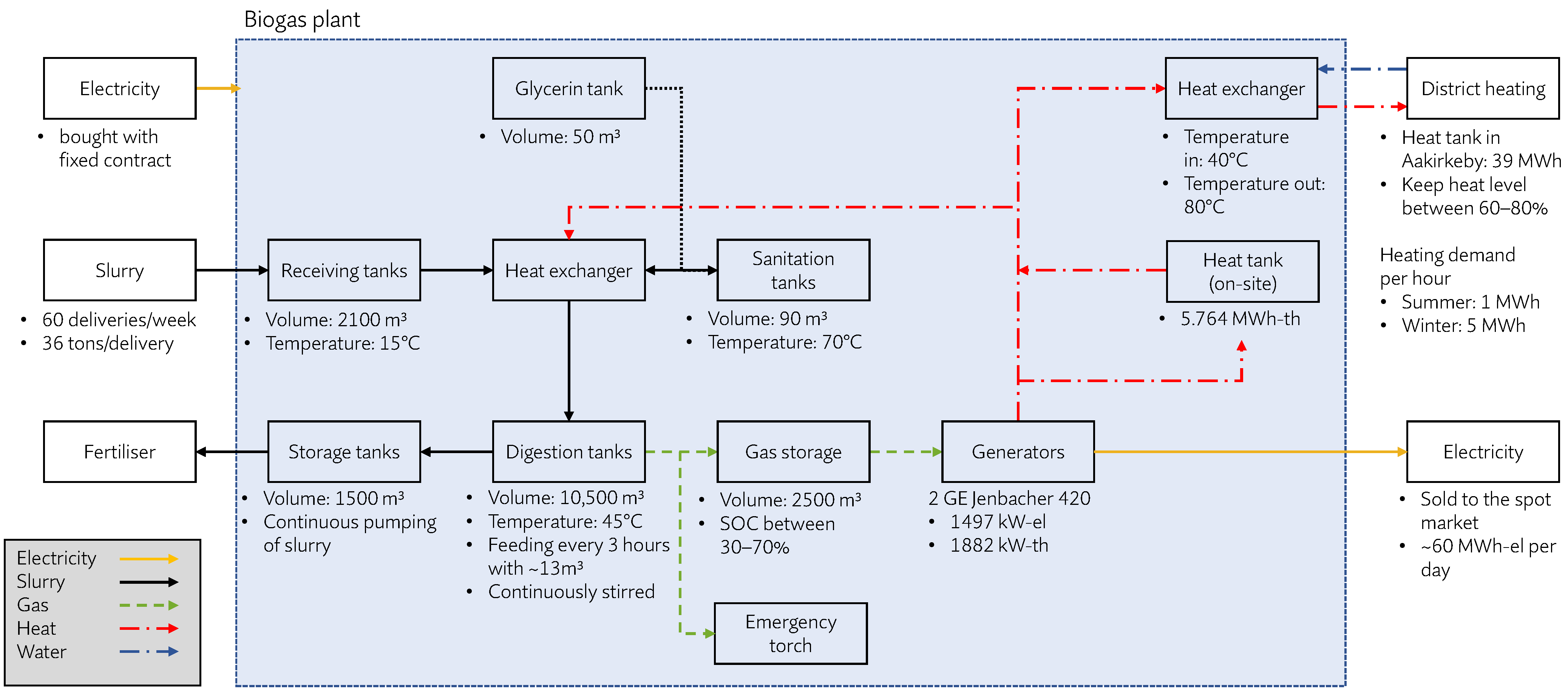
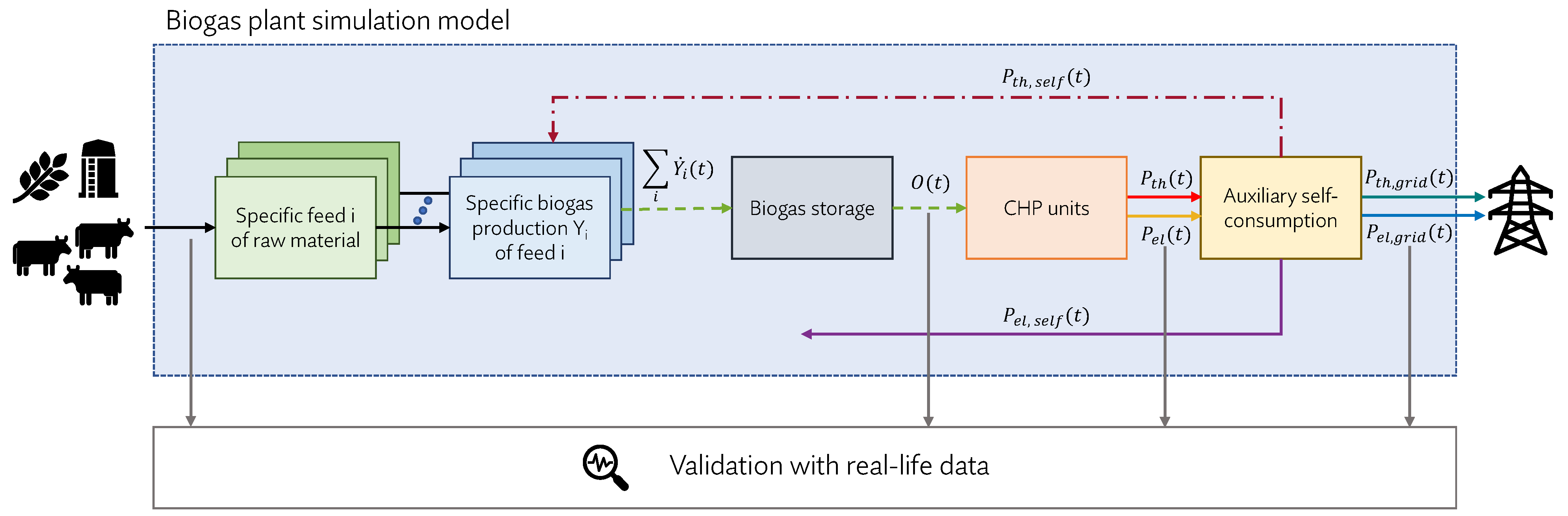
Figure 1 illustrates the procedures of the Bioenergi biogas plant on Bornholm in a block diagram with further information on each block. The following subsections successively describe the different parts of the Bioenergi biogas plant.

2.2. Feeding Management

The biogas production process starts with the delivery of slurry from local farmers on Bornholm that live in close vicinity to the plant. Deliveries take place around 60 times a week on working days, i.e., around 12 deliveries each day from Monday to Friday, with an average driving distance of 13.8 km. One delivery comprises on average 36 tons of, e.g., animal slurry or slaughterhouse waste. The average price the biogas plant has to pay is around 16 DKK per ton of slurry. 
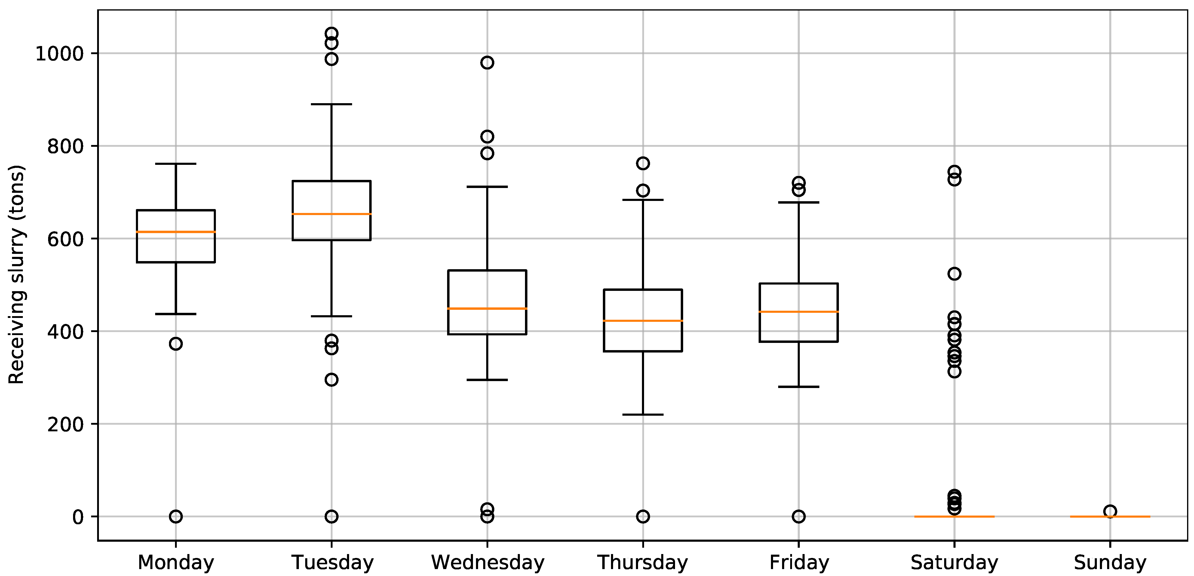
Figure 2 shows the boxplots of the daily received amounts of slurry created from data for a three-year time period between 1 January 2016 to 27 January 2019. By processing local organic waste, the biogas plant contributes to the island’s decarbonization strategy. In the current structure of the plant, the average substrate composition consists of 70.48% cow slurry, 19.82% of pig slurry, 6.17% of slaughterhouse waste, 3.30% of corn and 0.22% of fish waste, with an average percentage of total solids in the feedings of 12–14%. The island of Bornholm has a large feedstock potential both from animal husbandry, household wastes and secondary crops which is currently not fully exploited: from a total estimated amount of 741,425 tons the biogas plant currently has a permission to treat only 120,000 tons per year [16].
Next, the slurry is pumped from the arriving trucks into the receiving tanks, which are concrete tanks inset into the ground with a total capacity of 2100 m3. In the receiving tanks, the slurry has a temperature of around 15 °C. From there, a certain amount of the slurry is continuously pumped through a heat exchanger in the form of intertwined pipes into three sanitation tanks. In the heat exchanger, the slurry is heated to around 65–70 °C with the help of slurry fed back from the sanitation tanks and excess heat from the generators. The sanitation tanks have a total capacity of 90 m3 and the slurry remains approximately one hour in the sanitation step. In this way, populations of existing bacteria are eliminated that would otherwise interfere with the bacteria population inside the digestion tanks. Moreover, the pre-treatment breaks up the organic components in the slurry such that they are more easily digestible from the bacteria and hence a faster biogas production can be achieved. The heat exchanger not only heats the incoming slurry, but also simultaneously cools the treated slurry from the sanitation tanks which is then fed into the reactor tanks at a temperature of around 45 °C.
On the site, there are three reactor tanks with a total capacity of 10,500 m3, in which the slurry is digested by bacteria under anaerobic conditions. The feeding into the cylindrical reactor tanks takes place every three hours with a volume of approximately 13 m3, accumulating on average to 383 tons per day (in September 2020). The content of the reactor tanks is continuously stirred with a rotor connected to a centrally positioned vertical shaft. From the reactor tanks, a certain amount of slurry is continuously drawn out from the bottom of the tanks and pumped to the storage tanks for the degassed slurry. It is then fetched again by the farmers and used as fertilizers on local fields. The hydraulic retention time, i.e., the average time the material remains in the digestion tank, is 25 days.

2.3. Gas Storage Capacity and Control

The produced biogas is drawn from the top of the reactor tanks and sent through pipes to the gas storage. The gas pipes installed on-site are of the sizes DN200, DN225 and DN280 with respective lengths of 50 m, 20 m and 190 m, leading to a total volume of 550 m3 in the pipes. The on-site gas storage has a capacity of 2500 m3, while additional gas is concentrated in the three digester tanks (3 × 1000 m3). It is aimed at keeping the gas storage level between 40–70% to retain a level of flexibility in both directions, albeit violations to the targeted storage level may occur. An emergency torch is connected to the pipes which is used in case the gas storage reaches its upper limit and the pressure in the pipes becomes too high. The torch then burns excess biogas on the spot.
The gas storage is controlled manually. If more biogas is produced than the amount that can be burned in the gas engines, the amount of infeed is lowered. Vice versa, when the gas storage level is low, the amount of infeed is increased or the generator output lowered.

2.4. Electrical and Thermal Co-Generation of the Plant

Two generators are fed with biogas from the gas storage. The generators get electrical setpoints based on the amount of biogas produced in the process. All produced electricity is sold to the island’s energy system based on a subsidized feed-in tariff of approx. 111 € per MWh supplemented by a price surcharge of approx. 35 € per MWh. For comparison, the mean spot price in the bidding area DK2 for the year 2020 settled at 28.31 €/MWh. The produced electricity can be sold at a higher price than the one the biogas plant must pay for procuring electricity, so the internal electricity consumption for the pumps and the stirring is financially decoupled from the own production. Heat is produced as a byproduct of the electricity generation. Some of the heat is used internally to heat the slurry in the heat exchanger. Another part of the heat is stored in a local water heat tank with a storage capacity of approximately 6 MWh. The biogas plant also has a connection to the local district heating system. In summer, the hourly heating demand is around 1 MWh, while in winter around 5 MWh. Through another heat exchanger the incoming water temperature of the district heating is increased from around 40 °C to at least 80 °C and sent back to the district heating storage tank in Aakirkeby that has a thermal capacity of 60 MWh.
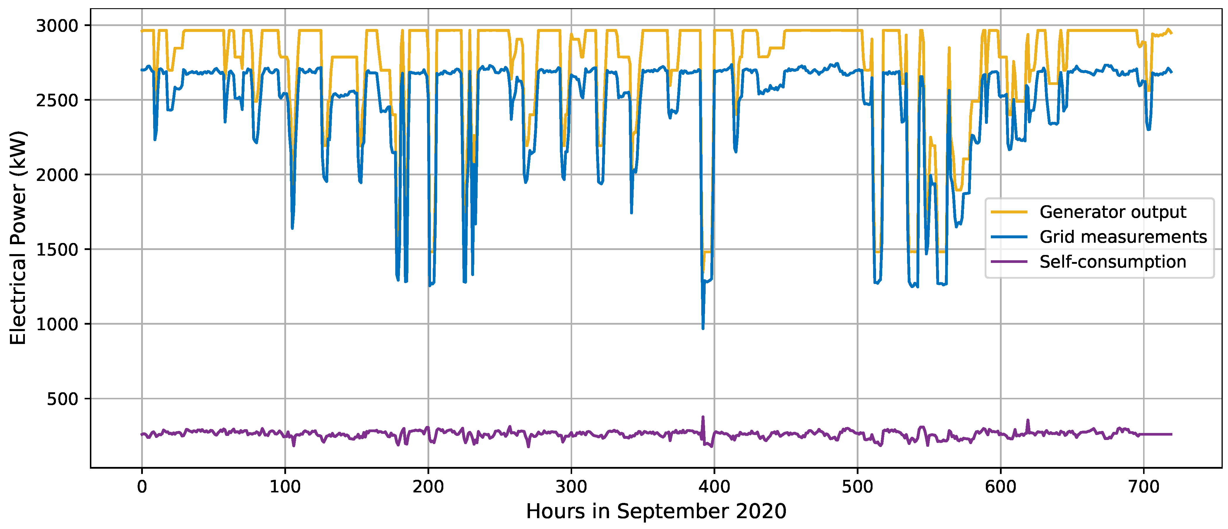
The biogas plant’s operations are energy-intensive. 
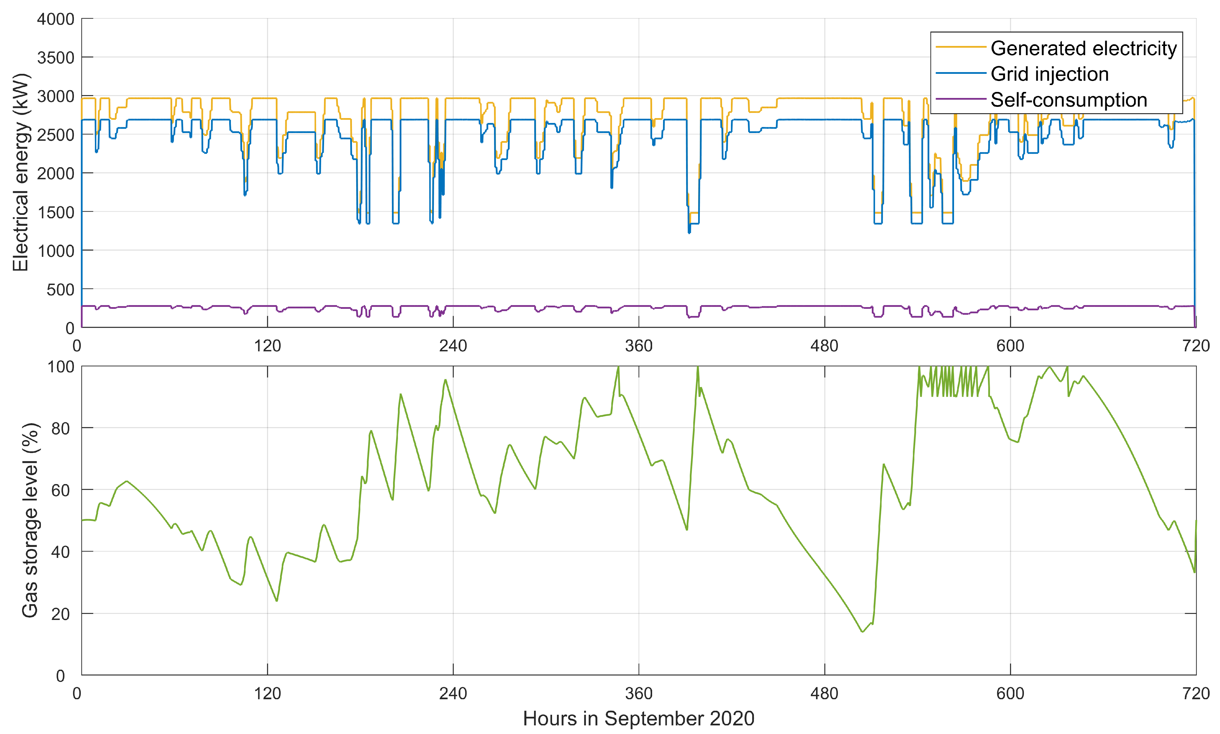
Figure 3 plots the measured electrical output of the generators together with measurements at the grid side and the derived electrical self-consumption of the plant in an hourly resolution for the month of September 2020. The biogas plant complex is the only consumer at this grid measurement. The figure thus exhibits that a close-to-constant electrical power of 260 kWel is needed for the plant’s electrical operations. This corresponds to a mean electrical self-consumption of the own production of 9.32%. Naegele et al. [17] and Akbulut [18] find similar magnitudes for full-scale biogas plants.
From the thermal energy perspective, a constant amount of heat is recirculated from the generators on site. On the one hand, the heat is directed to the heat exchangers heating the slurry that is pumped into the sanitation tanks from around 15 °C to up to 70 °C. On the other, the heat is used for keeping the digestion tanks at the operating temperature of 45 °C. This constant amount of thermal energy corresponds to 500 kWhth in one hour. Accordingly, around 12 MWh from the generated thermal energy remains on site which amounts to a thermal self-consumption of 14.7% for the month of September. In winter time, more thermal energy has be to recirculated on-site to be able to sustain the processes and heat the premises. For a 289 kW CHP unit, Akbulut [18] reports values of up to 45% of the own thermal energy generation over one year at an annual average outside temperature of 7.5 °C. In general, smaller biogas plants will face higher shares of self-consumption in relative terms. The thermal losses for smaller digestion tanks are disproportional to the losses for larger tank volumes. In addition, the auxiliary heat demand of the facilities of the plant do not scale linearly to the size of the units.

2.5. Heat-to-Power Ratio of the CHP Units

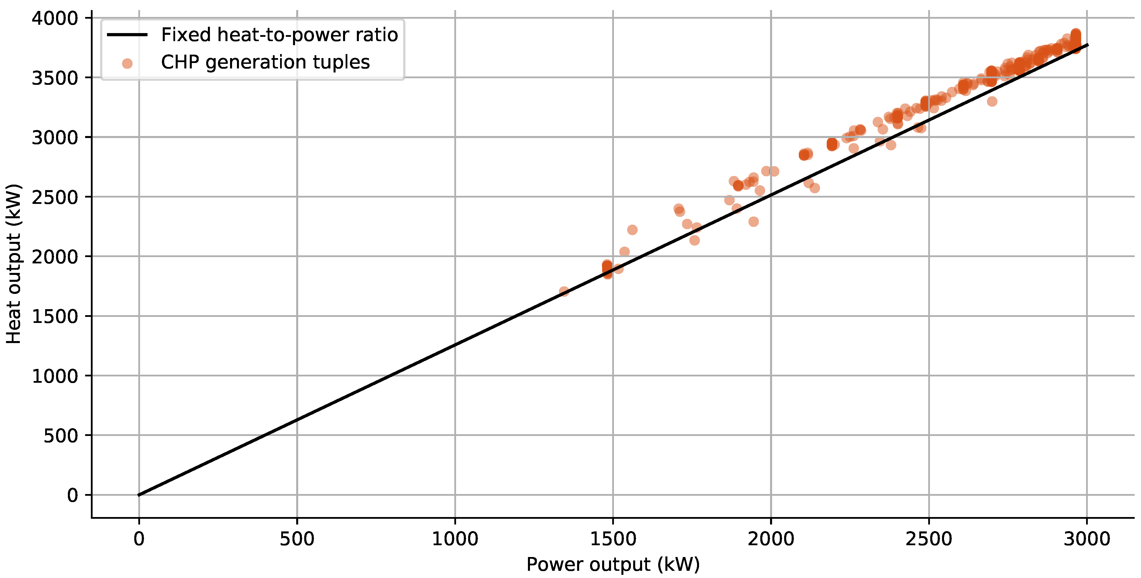
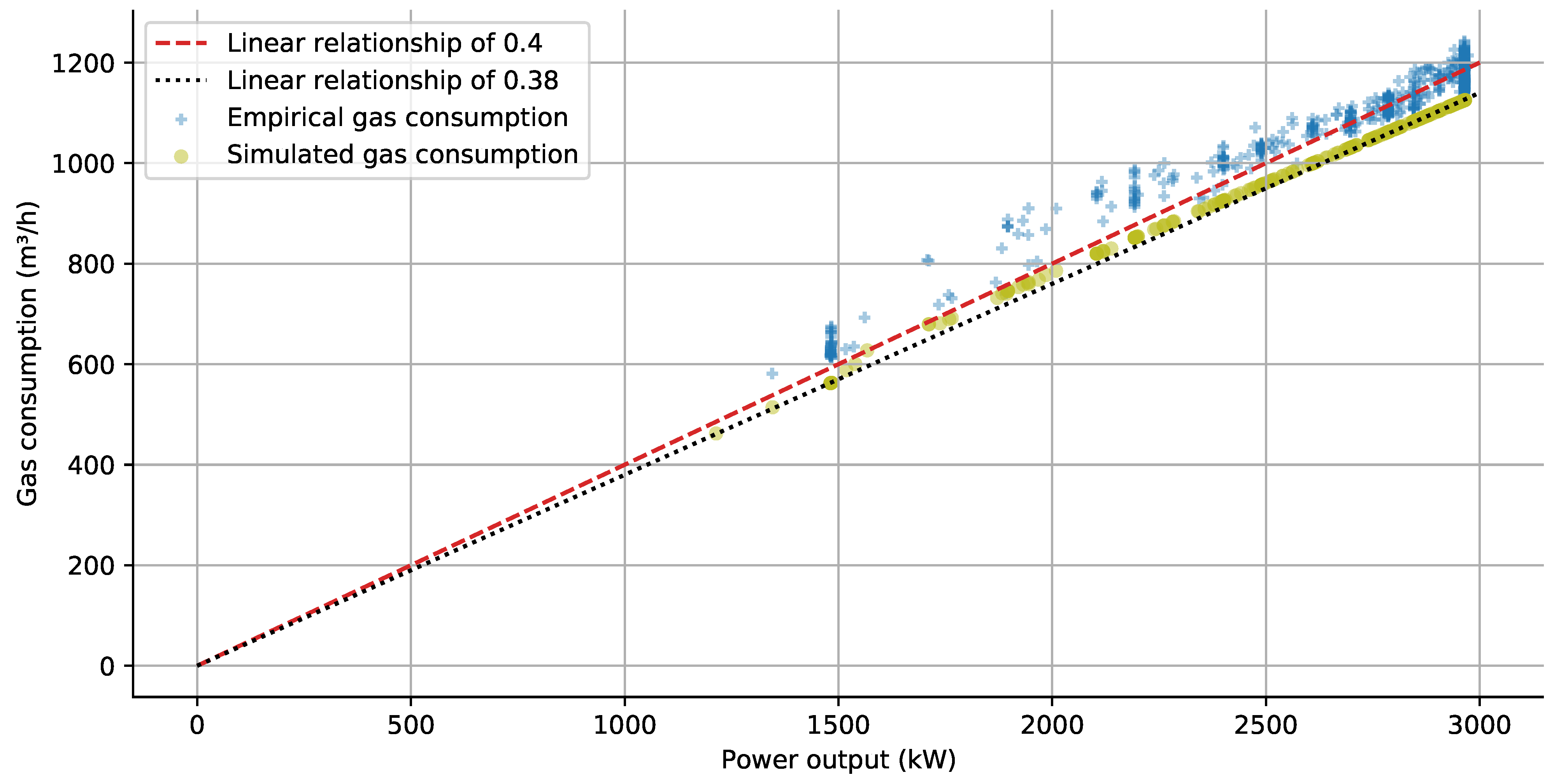
In an hourly resolution, there is a strong relationship between the generated heat and generated output power of the biogas plant. Figure 4 plots the hourly co-generation tuples for the month of September 2020 together with the fixed heat-to-power ratio reported in the generators’ datasheet. From the figure, it can be learned that the actual ratio might be slightly higher than reported, meaning that more heat is produced in hourly averages for a given hourly electrical output power. This might relate back to both inefficiencies in the burning process of the biogas as well as synergetic effects resulting in higher thermal output. From an electrical energy perspective, the heat-to-power ratio of the generators may thus be taken as a slight overestimate as more heat is generated at associated power values.

3. Methodology

The following section provides insights on the modeling approach for a biogas plant presented in this paper. It describes the main dynamic equations needed to estimate the transients for the anaerobic digestion process as well as the modeling of the gas storage and the CHP units. The model has been implemented in the MATLAB&Simulink environment and solves in a secondly time resolution.

3.1. Overview on the Modeling Approach

To model the complex biochemical process of a biogas plant with its anaerobic digestion processes coupled to the electrical and thermal energy generation, it is necessary to breakdown the simulation in smaller parts and make careful assumptions that simplify the modeling without compromising the dynamic behavior of the process. Figure 5 illustrates the modeling approach presented in this paper. Detailed theoretical background information and analysis of the biomass potential on the island of Bornholm are given in Zepter et al. [16]. The model takes daily or hourly time series of the infeed as input. Each time-amount tuple of the feeding is subsequently converted to a specific biogas production rate via the first-order derivative of a modified Gompertz function. The accumulated biogas production of the subsequent feedings is then fed into a biogas storage. The storage couples the biogas production and the gas consumption of (here two equally-sized) CHP units. Lastly, the thermal and electrical auxiliary self-consumption of the plant’s facilities are subtracted from the output of the generators for determining the magnitude of grid injections, both in terms of electrical and thermal energy. The following subsections describe the mathematical formulation behind these blocks which are based on the following assumptions and simplifications in the modeling approach:
  • The time resolution of the feeding schedule is amplified from three-hourly to daily feedings.
  • A constant substrate composition is assumed, while in reality the substrate composition would change slightly feed by feed.
  • The biochemical reactions inside the digestion tank are neglected and no sensitivities of, e.g., acidity level or temperature on the biogas production are assumed.
  • The relationship between pressure and volume in the gas storage has been neglected. All volumes are taken at atmospheric pressure.

3.2. Feeding

The first part of the model is connected to the feeding of raw material and organic waste. The biogas plant is mainly processing collected residuals from husbandry farmers on the island of Bornholm, as described in Section 2.2. It is assumed in this paper that the substrate composition of the feedings remains unchanged as no detailed information on the composition of the feedings is available. Hence, the shares of cattle slurry, pig slurry, slaughterhouse waste and corn silage are considered as 70%, 20%, 6% and 4%, respectively, close to what has been reported in Section 2.2. The utilization of fish waste is neglected here, due to the insignificant amounts. For this specific composition, the average amount of dry matter (DM) and subsequently volatile solids (VS) is calculated in Table 1.
The input for this first block of the model is the raw amount of slurry fed at a given point in time. This amount in wet weights is then multiplied with the average share of VS in the feeding material that may be processed to biogas by the use of microbial bacteria in the anaerobic digestion steps [19]. The biogas productivity correlates with the amount of organic matter or VS per ton fed slurry [20]. The time resolution of the feeding can be varied with the input table given to the model.

3.3. Biogas Production

The specific biogas production Y i ( t ) is based on a specific feeding instance i (Figure 5). The cumulative biogas production for such a feeding is in the literature often described either as a Monod-kinetic [23] or as a modified version of the Gompertz function [24]. The latter is a special case of a generalized logistic function where growth is characterized as being the slowest at the start and the end of a given time period. Equation (1) defines the specific version of the Gompertz function adapted for this model.
Y i ( t ) = F i · ϕ · exp exp μ m · e ϕ ( λ t ) + 1
F i is the organic fraction of the biomass feed i given in kg VS, ϕ = 0.7 is the biogas potential in m3 biogas per kg VS, μ m = 0.2 is the maximum biogas production rate in m3 biogas per kg VS and day, e is Euler’s number and λ = 4 is the input lag in days.
The marginal biogas production rate of a specific feed then follows the first-order derivative of the function given in Equation (1) with respect to the time t.
Y i ˙ ( t ) = F i · μ m · e · exp μ m · e ϕ ( λ t ) + 1 exp μ m · e ϕ ( λ t ) + 1
The total biogas production Y ˙ t o t in any point of time t [ 0 ; T ] is composed of the sum of the specific production rates of the subsequent feeding instances i I = 0 , , n , defined as
Y ˙ t o t ( t ) = i I Y ˙ i ( t ) = Y ˙ 1 ( t ) + Y ˙ 2 ( t ) + + Y ˙ n ( t ) ,
where n is the maximum number of simultaneously ongoing production rates which is dependent on the time resolution of the feeding.

3.4. Biogas Storage

The biogas storage (Figure 5) takes as input the sum of the ongoing production processes, which is the total biogas production rate of the plant in a specific point in time. The outflow of the biogas storage—the gas consumption of the generators—is depending on the reference setpoint of the CHP units. For a given electrical power reference P e l ( t ) , the outflow O ( t ) of the biogas storage can be calculated by considering the electrical efficiency of the generators η e l ( P e l ) as well as the methane share ( δ = 65 % ) in a m3 of biogas and energy content ( θ = 9.67 kWh) of a m3 methane, as defined in Equation (4).
O ( t ) = P e l ( t ) η e l ( P e l ) · θ · δ
The gas storage level L ( t ) as a percentage of the storage tank capacity σ s t o is hence depending on the biogas influx from the anaerobic digestion process, i.e., the total biogas production rate Y ˙ t o t ( t ) , and the outflow O ( t ) towards the CHP units, i.e., the gas consumption by the generators to fulfill a certain electrical setpoint. The dynamics of the gas storage level are represented by Equation (5). The initial gas storage level L i n i t at time t = 0 was set to 50% of the gas storage capacity σ s t o . The overall gas storage capacity of the biogas plant has been estimated to 6050 m3. It is assumed that besides the 2500 m3 gas storage tank, biogas can also be stored to a certain extent in the three digester tanks (1000 m3 each) and in the gas pipes (550 m3).
L ( t ) = 1 σ s t o Y ˙ t o t ( t ) O ( t ) d t + L i n i t
The upper and lower bounds of the storage are secured by a relay that switches off either the biogas intake or outtake once the respective boundary is violated, and resumes once a level of 90% or 10% of the storage is reached, respectively.

3.5. Combined Heat and Power Units

The modeling block for the two Jenbacher 420 co-generation units is structured from an electricity-led perspective. Thus, the model gets as input an hourly power reference signal for both CHP units and aims to fulfill these power requests by burning the necessary amount of biogas, as calculated in Equation (4). The CHP model considers an electrical efficiency of the generators η e l ( P e l ) as a function of their load level. For the characterization of the specific electrical part-load efficiency curve of one generator, a power function with rational exponents has been fitted to the data points given in its technical data sheet, as described by Equation (6) with α = 0.7012 , β = 0.0662 , γ = 0.3671 and P e l / P e l m a x [ 0 , 1 ] .
η e l ( P e l ) = 0.1 + γ · ( P e l / P e l m a x ) α ( P e l / P e l m a x ) α + β α
Considering empirical insights (Figure 4), it is a fair assumption to define the thermal part-load efficiency η t h ( P e l ) in this study by Equation (7) with the fixed heat-to-power ratio to the electrical efficiency η e l ( P e l ) , following the datasheet of the generators.
η t h ( P e l ) = 1.257 · η e l ( P e l )

3.6. Auxiliary Self-Consumption

The auxiliary electrical self-consumption of the biogas plant facility has been estimated based on measurements taken directly at the generators’ end and at the grid feeder connecting the biogas facilities (Figure 3). The electrical self-consumption is defined as the difference between the generator output power and the grid measurements. For the given month, the electrical energy consumed directly onsite amounts to γ e l , s e l f = 9.32% of the total generated electrical energy. Hence, the grid power P e l , g r i d ( t ) in the model is calculated as
P e l , g r i d ( t ) = ( 1 γ e l , s e l f ) · P e l ( t ) .
For estimating the thermal self-consumption of the plant, we rely on real-time data collected at the plant. The self-consumption can consequently be modeled by a steady recirculation of P t h , s e l f ( t ) = 0.5 MWhth in one hour. The thermal energy delivered to or stored for the district heating P t h , g r i d ( t ) is hence defined as
P t h , g r i d ( t ) = P t h ( t ) P t h , s e l f ( t ) .

4. Results

This section presents the results obtained from the biogas plant simulation for the month of September 2020. The model is solved with a variable step solver with a maximum step size of 360 s. The result section is divided into two parts. Section 4.1 is directed at the feeding management and the associated biogas generation, while Section 4.2 validates the model output in terms of gas consumption and energy generation against on-site measurements.

4.1. Feeding Management and Biogas Generation

In this study, a daily feeding schedule has been considered. Thus, it has been assumed that every day a specific amount of slurry is fed into the digestion tanks. Respectively, the biogas production rate is always connected to one specific day of feeding. Section 5 will provide a comprehensive discussion of the taken assumptions on the modeling results. For simulating a continuous operation of the plant, the feeding schedule and its associated biogas production had to be started up before the beginning of the investigated month. For this reason, the starting date of the model is mid-August 2020 so that the biogas production processes with its long time constants can attain a (rather) constant biogas production level.
Figure 6 illustrates the biogas production from a daily feeding schedule. The upper plot of Figure 6 visualizes the daily feeding instances in wet weights, marked in blue, together with the daily mean of 383 tons, measured throughout the whole month of September 2020 and plotted as a dashed red line. The evolution of the ongoing biogas production processes from each of the specific feeding instances for the first two weeks of the month of September 2020, following Equation (2), are displayed in the second subplot of Figure 6. It can be seen that for a specific feeding instance (see, e.g., the highlighted dashed blue line), the biogas production rate increases exponentially until it reaches its maximum rate, approximately with a time delay of five days. Subsequently, the biogas production rate decays exponentially over a longer time period. It can be seen from the plot that the biogas production of one specific feed spans approximately over a time period of 10–15 days. The third subplot of Figure 6 displays the associated cumulative biogas production of the feeding instances. It follows the sigmoidal Gompertz function described in Equation (1) where the slope of the increase is the highest, when a specific biogas production rate reaches its maximum.
The fourth subplot of Figure 6 aggregates the different ongoing biogas production rates into the total aggregated biogas production of all feeding instances, following Equation (3). The range of 0.28–0.32 m3/s corresponds to a gas flow rate of approximately 1008–1152 m3/h, resulting in a daily biogas production of around 25,000 m3 per day, and hence 750,000 m3 per month. For the 15 days displayed, the aggregated cumulative biogas production amounts to 381,000 m3.

4.2. Gas Consumption and Energy Output of the Generators

A first step of validating the accuracy of the presented biogas plant model is to look at the gas consumption of the two CHP generation units. Figure 7 plots the real and simulated hourly gas consumption of the engines against their hourly power output. The real gas consumption is measured on-site in two minute intervals and here aggregated to hourly values, while the simulated biogas consumption is calculated according to Equation (4). From the figure, it can be seen that the model is slightly underestimating the gas consumption of the engines. This might be due to the fact that there could in reality be further deviations in the quality of the biogas (e.g., lower share of methane), imperfections in the burning process as well as small gas leakages. However, looking at the two linear relationship coefficients that describe the gas consumption well at higher loading of the generators, their difference indicates a deviation of 5% between the interpolation of the real and simulated gas consumption of the plant.
Figure 8 plots the electrical energy output of the plant for the month of September 2020. The hourly setpoint given to the model can be satisfied at all times, while the level of grid injection and the self-consumption of the plant can be determined with high accuracy. Comparing Figure 8 to the empirical insights from Figure 3, it can be noted that the differences in the grid injection and self-consumption of the plant lie in the small deviations of the self-consumption that the model does not capture in detail. In terms of overall energy injections into the grid, the model estimates based on the hourly reference setpoint grid injections of accumulated 1779 MWhel for the entire month, while the real grid injections add up to 1776.42 MWh. The difference between the two signify an overestimation of 0.15% in terms of electrical energy grid injections. Regarding the electrical self-consumption, the simulation model underestimates the self-consumption of the plant by 3.1%, amounting to a total monthly self-consumption of 182.7 MWh, while the empirical evidence indicates a value of 188.6 MWh. The mean power value of the self-consumption amounts to 253.8 kW, while the real data suggest a value of 261.9 kW on average.
The model simulated a monthly thermal generation of 2464 MWh, while the measured value from the biogas plant amounted to 2448 MWh. Hence, the model slightly overestimates the thermal generation of the plant by 0.65%. From the 2464 MWh that the biogas plant produced in the model, a total amount of 359.2 MWh was used directly on-site. The thermal self-consumption therefore amounts to 14.58% which is 0.12% less than what has been calculated from the on-site measurements. All in all, these differences are insignificant.
The simulated gas storage level is depicted in the lower plot of Figure 8. It can be seen that the simulated gas storage level is well filled for most of the simulation time, providing flexibility for the co-generation of the CHP units. In some occasions, the storage level hits the upper bound of the simulated low-pressure gas storage tank. It might be possible that the biogas plant in these times was asked by the network operator to decrease its electrical output. Hence, not all of the biogas could be used and was subsequently burned in the emergency torch of the plant. However, it might also be the case that the model does not capture the biogas generation well enough which will be discussed in the following section.

5. Discussion

In general, the presented results suggest that the dynamic behavior of a biogas plant can be reproduced with sufficient accuracy. The model is able to determine the thermal energy output and self-consumption of the plant as well as the biogas production based on daily feeding instances of raw materials. The first part of this section reviews and challenges the assumptions made in constructing this model. The second part is devoted to an analytical discussion of how the biogas plant can come into focus for the production of alternative fuels.

5.1. Limitations of the Modeling Approach

Step by step, it will be assessed how far the simulation results of the model would change when considering (i) different time resolutions of the feeding, (ii) a dynamic substrate composition, (iii) biochemical interactions in continuously stirred digestion tanks and (iv) a pressure–volume dependency in the gas storage. Lastly, required modifications of the model are discussed to apply it to other months or other biogas plants.

5.1.1. Time Resolution of the Feeding

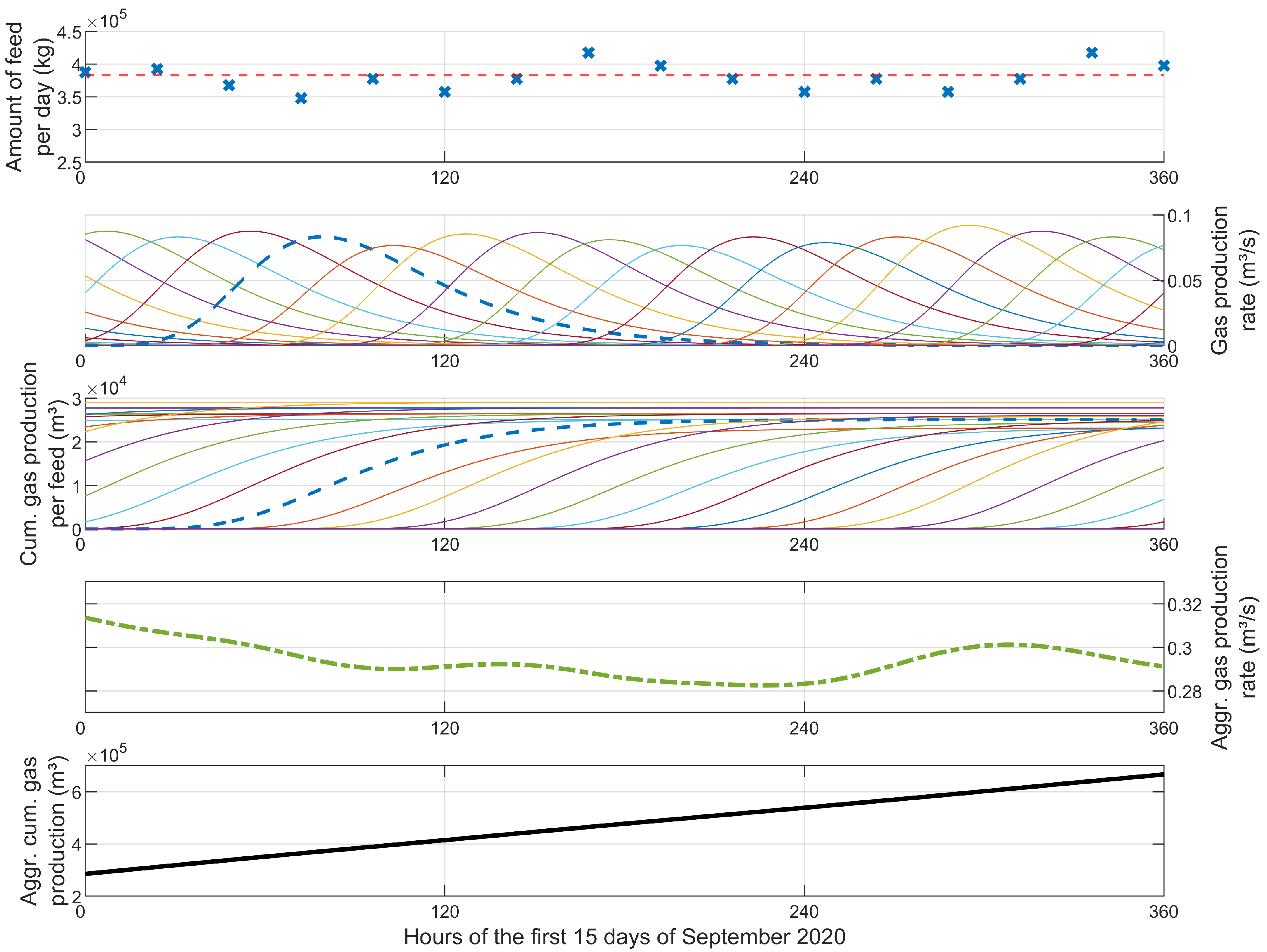
In reality, the Bioenergi biogas plant is fed every three hours for 37 min with a volume flow of 21 m3 per hour. In the model, this has been simplified to daily instantaneous feedings. The model is not structured to take into account the biochemical reactions to the largest extent, since it is rather directed at disclosing the time constants associated with a feed and its associated biogas production. In addition, there is no comprehensive information on the amount of the single feedings. If an equal amount is fed every 24 h, every 8 h or even every three hours, from the pure perspective of the considered dynamics, the overall biogas production will change insignificantly. Hence, a daily feeding results in a good approximation, i.e., a rather constant biogas production, of a feeding schedule every three hours. This is however depending on the amount of the feeding. If the amount of feedings varies significantly in the three hour feeding schedule, e.g., one larger feed followed by a sequence of smaller feedings, then the wave motion of the biogas production will adjust. In the end, the choice of time resolution depends largely on the level of accuracy that is envisioned in the modeling process. Here, the considered dynamics of a daily feeding are accurate enough to fulfill hourly electrical setpoints. If faster dynamics are of interest, it may be necessary to convert to a three-hour feeding schedule. For example, this could apply when using the biogas plant for providing primary frequency control, where the fast frequency dynamics would require quick changes in the power output. For this specific type of study, the gas storage modeling assumes a larger importance due to the possibility of the buffering for providing the necessary flexibility required by the frequency control without compromising the feeding process.

5.1.2. Dynamic Substrate Composition

A dynamic adjustment of the substrate composition would increase the precision of the model in matching the real values significantly. However, no exhaustive information regarding the substrates are associated with the feeding amount. Hence, from a modeling perspective, the average value of the substrate composition has to serve as the closest possible representation. By dynamically adjusting the substrate composition of the feedings, the biogas potential as well as the share of VS would change dynamically as well. This would lead to a closer representation of the single biogas production rate associated to each feeding, but for the present biogas plant this information is not available.

5.1.3. Biochemical Reactions in the Digester

In a continuously stirred digestion tank, there are biochemical reactions that have an impact on the biogas productivity of the microbial bacteria population. Biochemical interdependencies are not taken into account in this modeling approach as they would specify a level of detail that is out of scope of this analysis. In the same light, sensitivity of the substrate composition or feeding times on the bacteria population is neglected. It is further assumed that the temperature as well as the acidity level (pH-value) is kept constant at an optimal level for the bacteria throughout the digestion process and that they have no influence on the biogas productivity. The modeling of the anaerobic digestion part hence reduces to a mere dynamic process. For a more in-depth representation of these processes, kinetics models such as presented in by Nopharatana et al. [25] and Rosen et al. [26] should be considered. Different modeling approaches of anaerobic digestion have been reviewed by Kythreotou et al. [27], while Heiker et al. [28] performed a systematic comparison of modeling approaches of biogas production in the context of energy system and process optimization models. The taken simplifications could, e.g., result in a flawed estimation of the biogas production which would contribute to explain the gas storage level evolution depicted in Figure 8.

5.1.4. Pressure–Volume Dependency

According to Boyle’s law, the volume of a gas is inversely proportional to the pressure at constant temperature. Hence, the amount of gas that can be stored in, e.g., a gas tank or in pipes, may be increased by enhancing the pressure level. This dependency is not taken into account which has a strong effect on the presented results. In the lower plot of Figure 8, the evolution of the biogas storage is presented. It can be seen that the biogas storage level hits in multiple occasions the upper bound. It could be speculated that this has not been happening in reality as the targeted range in which the biogas storage is operated is between 40–70%, according to information from the plant. By introducing a pressure–volume dependency, the evolution of the gas storage level will be compressed more towards the mid-range of the storage capacity, and consequently not collide with the storage boundaries.

5.1.5. Generalization of the Model

Due to limited data availability from the plant, the model has been fitted to and validated for the month of September 2020. The proposed modeling approach allows, however, for the application of the presented model to other months, if feeding instances and electricity reference setpoints are adjusted. Although tailored to one specific biogas plant, the model may also represent other biogas plants if the utilized substrates and their associated biogas production parameters (e.g., biogas potential and maximum production rate) as well as the characteristics of the plant (e.g., generator size, tank volumes) are modified.

5.2. Assessment of Biogas Upgrading Opportunities

Biogas plants play a vital role in multi-energy systems since they provide—besides their low-carbon co-generation of electricity and hea—the possibility of upgrading biogas to synthetic natural gas (SNG) [29]. The generated SNG can hence be injected into the natural gas grid or liquefied for the transportation sector (e.g., heavy-road or maritime transport). Moreover, biogas plants represent a compelling site choice for power-to-gas and methanization facilities as they offer connections to DHNs which increases the energy efficiency of the conversion processes. Within the Insulae project, the role of a biogas plant is investigated as part of a multi-domain virtual power plant. This section analytically reviews the potential for biogas upgrading at the Bioenergi biogas plant on the island of Bornholm from a pure energy perspective. Due to its high efficiency at elevated temperatures and possible utilization of waste heat, the catalytic methanization of biogas via hydrogenation is examined. Based on a Sabatier reaction, biogas is enriched with hydrogen (H2) for converting its share of carbon dioxide (CO2) to methane (CH4). The investigation and comparison of alternative upgrading technologies (e.g., CO2 removal by physical or biological methods) has not been carried out in this paper and remains for further research. A review of current and prospective biogas upgrading technologies has been performed by Angelidaki et al. [30].
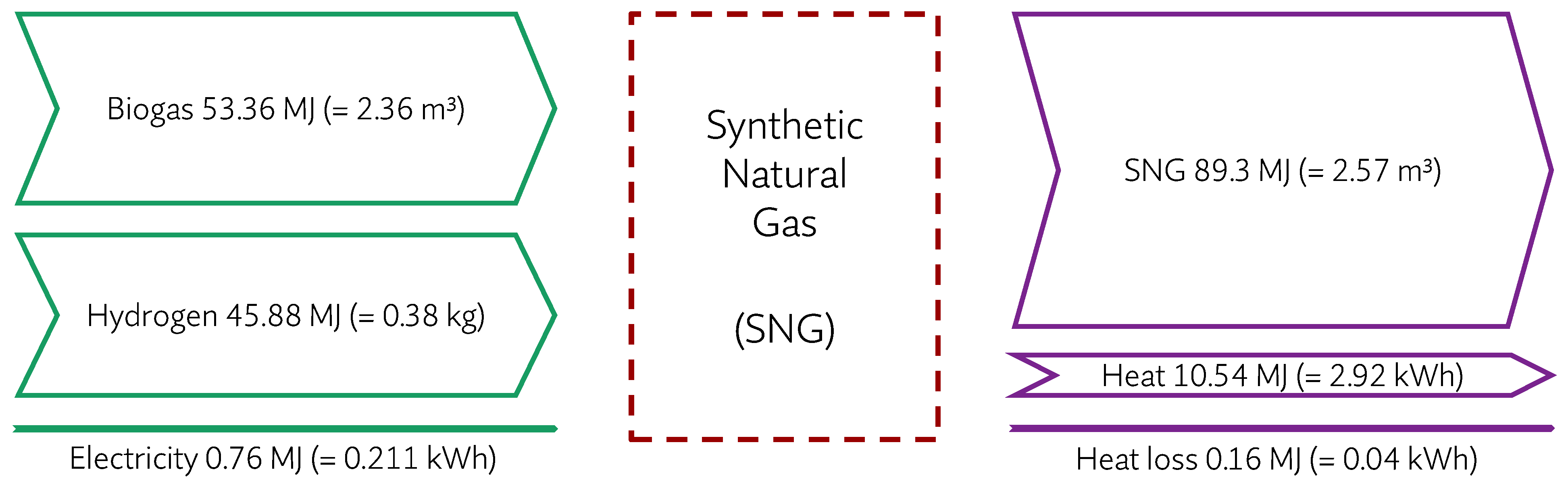
Following the energy balance presented by the Danish Energy Agency and Energinet [31] illustrated in Figure 9, a methanization process via the hydrogenation of biogas requires besides a small share of electricity (0.76% of the input energy in MJ) a larger share of hydrogen (45.88% of the input energy in MJ). The remaining 53.36% of the input energy is stored in the biogas. If it is intended to transform the monthly biogas production of 750,000 m3 from the plant into SNG, approximately 121 tons of hydrogen and 67 MWh of electricity are needed, following the above stated ratio in terms of energy. The production of 121 tons of hydrogen requires in one month 6655 MWh of electrical energy, assuming an efficiency of 55 kWh/kg H2 in an electrolysis process [32,33]. For one month of 30 days, this would require an electrolyzer of 9.2 MW to be run at nominal power throughout the whole month.
Then, out of 750,000 m3 biogas, a total amount of 815,929 m3 of SNG may be produced. While the total energy that can be retrieved from 750,000 m3 of biogas with an assumed energy content of 6.5 kWh/m3 is 4875 MWh, the upgraded amount of SNG holds an energy content of approximately 8135 MWh, considering 9.97 kWh/m3. The energy content of the biogas corresponds to the energy requirement of the generators running at 95% of nominal power throughout the month. From the produced SNG, only 62.7% could be directly utilized in the generators running at full load. The remaining 37.3% (3034 MWh; 304,349 m3) of the SNG production can be used either for transportation or other energy requirements. It is noteworthy that the gained 3034 MWh stored in the SNG in relation to the additional 6655 MWh needed for the electrolysis process result in an efficiency of 45.59% for this conversion process. The monthly energy requirement for the electrolysis process is three times higher than the biogas plant’s electrical energy production. To this end, it would be important to couple the electrolysis process with surrounding large-scale renewable energy sources such as wind and PV farms where excess generation in case of grid overloading may be used for hydrogen generation. However, it is unlikely that this will result in a constant 9 MW power flow throughout the month.

6. Conclusions

Biogas plants offer solutions to the challenges that arise from the green energy transformation. They provide dispatchable electricity generation necessary for grid balancing of renewable energy systems, and entail potentials for biogas upgrading and conversion to alternative fuels, e.g., in case of an oversupply of variable renewable energy. This paper gathers empirical insights on the functioning of a biogas plant on the island of Bornholm, Denmark. A simulation model for representing the relevant dynamics of the internal processes of a biogas plant has been developed and validated against historical measurements from the plant. The model considers the transients of the anaerobic digestion based on first-order kinetics, the gas storage, the CHP units, as well as the auxiliary self-consumption of the complex. The simulation results match the historical measurements with high accuracy. Hence, the model may be able to characterize the functioning of the plant also for unknown power requests.
The influence of made assumptions regarding the time resolutions of the feeding, dynamic substrate composition, simplifications of biochemical reactions and neglected pressure–volume dependency on the simulation results has been discussed in detail. With the approximations of the biochemical reactions in the anaerobic digestion, the model does not aim at the highest accuracy in the biogas production process, but it gives an estimate of the relationship between feeding management and biogas production that can be utilized for flexibility provision towards the electrical and thermal networks. Future work will be directed at the enhancement of a virtual power plant in combination with adjacent wind and PV farms where the flexibility of the biogas plant will be exploited for providing grid services. The here presented model can thus be used to develop control strategies for virtual power plants comprising a biogas plant.
Furthermore, the paper discusses the potentials for biogas upgrading via hydrogenation at this specific plant from a pure energy perspective, i.e., neglecting the necessary infrastructure and process dynamics of the conversion. Hence, the amount of hydrogen needed can be estimated and put in relation to the gained energy output of biomethane. From an energy efficiency perspective, it can be concluded that the process is connected to high losses that compromise the viability of the conversion. Further research needs to be conducted to investigate the potentials of alternative fuels that can be derived from biogas for decarbonizing, e.g., the transport or industry sector.

Author Contributions

Conceptualization, J.M.Z., J.E., T.G. and M.M.; methodology, J.M.Z., J.E., T.G. and M.M.; software, J.M.Z.; formal analysis, J.M.Z.; investigation, J.M.Z.; writing—original draft preparation, J.M.Z.; writing—review and editing, J.M.Z., J.E., T.G. and M.M.; visualization, J.M.Z.; supervision, T.G. and M.M.; funding acquisition, M.M. All authors have read and agreed to the published version of the manuscript.

Funding

This work has received funding from the H2020 INSULAE project under the Grant Agreement No. 824433. The goal of the project is to provide innovative energy solutions for decarbonizing European islands. For more information, visit http://insulae-h2020.eu/, accessed on 8 October 2020.

Conflicts of Interest

The authors declare no conflict of interest.

Abbreviations

The following abbreviations, variables and parameters are used in this manuscript:
CH4Methane
CHPCombined heat and power
CO2Carbon dioxide
DHNDistrict heating network
DMDry matter
H2Hydrogen
PVPhotovoltaics
SNGSynthetic natural gas
VSVolatile solids
Variables
FOrganic fraction of feed (kg VS)
YSpecific biogas production (m3)
Y ˙ Specific biogas production rate (m3/s)
OOutflow of the biogas storage (m3/s)
LGas storage level (%)
P e l Electricity generation of CHP units (kW)
P t h Thermal generation of CHP units (kW)
P e l , g r i d Electricity grid injection (kW)
P t h , g r i d Thermal grid injection (kW)
Parameters
ϕ Biogas potential (m3 biogas per kg VS)
μ m Maximum production rate (m3 biogas per kg VS and day)
λ Input lag (days)
η e l Electrical efficiency of CHP unit (%)
η t h Thermal efficiency of CHP unit (%)
θ Energy content of methane (kWh per m3)
δ Share of methane in biogas (m3 methane per m3 biogas)
σ s t o Gas storage capacity (m3)
L i n i t Initial gas storage level (% of σ s t o )
γ e l , s e l f Share of electrical self-consumption (%)
P t h , s e l f Thermal self-consumption (kW)

References

  1. Haas, J.; Cebulla, F.; Cao, K.; Nowak, W.; Palma-Behnke, R.; Rahmann, C.; Mancarella, P. Challenges and trends of energy storage expansion planning for flexibility provision in low-carbon power systems—A review. Renew. Sustain. Energy Rev. 2017, 80, 603–619. [Google Scholar] [CrossRef] [Green Version]
  2. Lauer, M.; Thrän, D. Flexible Biogas in Future Energy Systems—Sleeping Beauty for a Cheaper Power Generation. Energies 2018, 11, 761. [Google Scholar] [CrossRef] [Green Version]
  3. European Commission. A Hydrogen Strategy for a Climate-Neutral Europe; European Commission: Brussels, Belgium, 2020. [Google Scholar]
  4. Scarlat, N.; Dallemand, J.F.; Fahl, F. Biogas: Developments and perspectives in Europe. Renew. Energy 2018, 129, 457–472. [Google Scholar] [CrossRef]
  5. Dotzauer, M.; Pfeiffer, D.; Lauer, M.; Pohl, M.; Mauky, E.; Bär, K.; Sonnleitner, M.; Zörner, W.; Hudde, J.; Schwarz, B.; et al. How to measure flexibility—Performance indicators for demand driven power generation from biogas plants. Renew. Energy 2019, 134, 135–146. [Google Scholar] [CrossRef]
  6. Mauky, E.; Jacobi, H.F.; Liebetrau, J.; Nelles, M. Flexible biogas production for demand-driven energy supply–feeding strategies and types of substrates. Bioresour. Technol. 2015, 178, 262–269. [Google Scholar] [CrossRef]
  7. Mauky, E.; Weinrich, S.; Jacobi, H.F.; Nägele, H.J.; Liebetrau, J.; Nelles, M. Demand-driven biogas production by flexible feeding in full-scale—Process stability and flexibility potentials. Anaerobe 2017, 46, 86–95. [Google Scholar] [CrossRef]
  8. Mauky, E.; Weinrich, S.; Nägele, H.J.; Jacobi, H.F.; Liebetrau, J.; Nelles, M. Model Predictive Control for Demand-Driven Biogas Production in Full Scale. Chem. Eng. Technol. 2016, 39, 652–664. [Google Scholar] [CrossRef]
  9. Gu, C.; Xie, D.; Sun, J.; Wang, X.; Ai, Q. Optimal Operation of Combined Heat and Power System Based on Forecasted Energy Prices in Real-Time Markets. Energies 2015, 8, 14330–14345. [Google Scholar] [CrossRef]
  10. Theuerl, S.; Herrmann, C.; Heiermann, M.; Grundmann, P.; Landwehr, N.; Kreidenweis, U.; Prochnow, A. The Future Agricultural Biogas Plant in Germany: A Vision. Energies 2019, 12, 396. [Google Scholar] [CrossRef] [Green Version]
  11. Korberg, A.D.; Skov, I.R.; Mathiesen, B.V. The role of biogas and biogas-derived fuels in a 100% renewable energy system in Denmark. Energy 2020, 199, 117426. [Google Scholar] [CrossRef]
  12. Gabderakhmanova, T.; Engelhardt, J.; Zepter, J.M.; Sørensen, T.M.; Boesgaard, K.; Ipsen, H.H.; Marinelli, M. Demonstrations of DC microgrid and virtual power plant technologies on the Danish island of Bornholm. In Proceedings of the 2020 55th International Universities Power Engineering Conference (UPEC), Turin, Italy, 1–4 September 2020; pp. 1–6. [Google Scholar] [CrossRef]
  13. Bornholms Regionskommune. Welcome to Bornholm, Bright Green Island. 2019. Available online: www.brightgreenisland.dk (accessed on 22 April 2021).
  14. Geissdoerfer, M.; Savaget, P.; Bocken, N.M.; Hultink, E.J. The Circular Economy—A new sustainability paradigm? J. Clean. Prod. 2017, 143, 757–768. [Google Scholar] [CrossRef] [Green Version]
  15. Schroeder, P.; Anggraeni, K.; Weber, U. The Relevance of Circular Economy Practices to the Sustainable Development Goals. J. Ind. Ecol. 2019, 23, 77–95. [Google Scholar] [CrossRef] [Green Version]
  16. Zepter, J.M.; Gabderakhmanova, T.; Andreasen, K.M.; Boesgaard, K.; Marinelli, M. Biogas plant modelling for flexibility provision in the power system of Bornholm island. In Proceedings of the 2020 55th International Universities Power Engineering Conference (UPEC), Turin, Italy, 1–4 September 2020; pp. 1–6. [Google Scholar] [CrossRef]
  17. Naegele, H.J.; Lemmer, A.; Oechsner, H.; Jungbluth, T. Electric Energy Consumption of the Full Scale Research Biogas Plant “Unterer Lindenhof”: Results of Longterm and Full Detail Measurements. Energies 2012, 5, 5198–5214. [Google Scholar] [CrossRef]
  18. Akbulut, A. Techno-economic analysis of electricity and heat generation from farm-scale biogas plant: Çiçekdağı case study. Energy 2012, 44, 381–390. [Google Scholar] [CrossRef]
  19. Ahring, B.K. Biomethanation I: Perspectives for Anaerobic Digestion. In Advances in Biochemical Engineering/Biotechnology; Springer: Berlin, Germany; London, UK, 2003. [Google Scholar]
  20. Triolo, J.M.; Ward, A.J.; Pedersen, L.; Sommer, S.G. Characteristics of Animal Slurry as a Key Biomass for Biogas Production in Denmark. In Biomass Now—Sustainable Growth and Use; Matovic, M.D., Ed.; InTech: London, UK, 2013. [Google Scholar] [CrossRef] [Green Version]
  21. Linke, B.; Muha, I.; Wittum, G.; Plogsties, V. Mesophilic anaerobic co-digestion of cow manure and biogas crops in full scale German biogas plants: A model for calculating the effect of hydraulic retention time and VS crop proportion in the mixture on methane yield from digester and from digestate storage at different temperatures. Bioresour. Technol. 2013, 130, 689–695. [Google Scholar] [CrossRef] [PubMed]
  22. Olesen, J.E.; Møller, H.B.; Petersen, S.O.; Sørensen, P.; Nyord, T.; Sommer, S.G. Bæredygtig Biogas: Klima- og Miljøeffekter af Biogasproduktion; DCA—Nationalt Center for Fødevarer og Jordbrug, Aarhus Universitet: Tjele, Denmark, 2020. [Google Scholar]
  23. Saeed, M.; Fawzy, S.; El-Saadawi, M. Modeling and simulation of biogas-fueled power system. Int. J. Green Energy 2019, 16, 125–151. [Google Scholar] [CrossRef]
  24. Córdoba, V.; Fernández, M.; Santalla, E. The effect of substrate/inoculum ratio on the kinetics of methane production in swine wastewater anaerobic digestion. Environ. Sci. Pollut. Res. Int. 2018, 25, 21308–21317. [Google Scholar] [CrossRef] [PubMed]
  25. Nopharatana, A.; Pullammanappallil, P.C.; Clarke, W.P. Kinetics and dynamic modelling of batch anaerobic digestion of municipal solid waste in a stirred reactor. Waste Manag. 2007, 27, 595–603. [Google Scholar] [CrossRef]
  26. Rosen, C.; Vrecko, D.; Gernaey, K.V.; Pons, M.N.; Jeppsson, U. Implementing ADM1 for plant-wide benchmark simulations in Matlab/Simulink. Water Sci. Technol. 2006, 54, 11–19. [Google Scholar] [CrossRef] [Green Version]
  27. Kythreotou, N.; Florides, G.; Tassou, S.A. A review of simple to scientific models for anaerobic digestion. Renew. Energy 2014, 71, 701–714. [Google Scholar] [CrossRef]
  28. Heiker, M.; Kraume, M.; Mertins, A.; Wawer, T.; Rosenberger, S. Biogas Plants in Renewable Energy Systems—A Systematic Review of Modeling Approaches of Biogas Production. Appl. Sci. 2021, 11, 3361. [Google Scholar] [CrossRef]
  29. Götz, M.; Lefebvre, J.; Mörs, F.; McDaniel Koch, A.; Graf, F.; Bajohr, S.; Reimert, R.; Kolb, T. Renewable Power-to-Gas: A technological and economic review. Renew. Energy 2016, 85, 1371–1390. [Google Scholar] [CrossRef] [Green Version]
  30. Angelidaki, I.; Treu, L.; Tsapekos, P.; Luo, G.; Campanaro, S.; Wenzel, H.; Kougias, P.G. Biogas upgrading and utilization: Current status and perspectives. Biotechnol. Adv. 2018, 36, 452–466. [Google Scholar] [CrossRef] [PubMed] [Green Version]
  31. Danish Energy Agency; Energinet. Technology Data for Renewable Fuels: Technology Descriptions and Projections for Long-Term Energy system planning. Catalogue on Technologies for Energy Carrier Generation and Conversion. 2017; (updated 2021). Available online: https://ens.dk/sites/ens.dk/files/Analyser/technology_data_for_renewable_fuels.pdf (accessed on 22 April 2021).
  32. Buttler, A.; Spliethoff, H. Current status of water electrolysis for energy storage, grid balancing and sector coupling via power-to-gas and power-to-liquids: A review. Renew. Sustain. Energy Rev. 2018, 82, 2440–2454. [Google Scholar] [CrossRef]
  33. Matute, G.; Yusta, J.M.; Correas, L.C. Techno-economic modelling of water electrolysers in the range of several MW to provide grid services while generating hydrogen for different applications: A case study in Spain applied to mobility with FCEVs. Int. J. Hydrogen Energy 2019, 44, 17431–17442. [Google Scholar] [CrossRef]
Figure 1. Block diagram of the biogas plant’s processes.
Energies 14 02424 g001
Figure 2. Weekly receiving schedule for slurry for data from 1 January 2016, to 27 January 2019. The boxes span from the 25% to the 75% quartiles and the respective median is given as orange line, while the whiskers extent to maximum 1.5 times the interquartile range. The remaining points are given as outliers.
Energies 14 02424 g002
Figure 3. Electricity production of the generators (yellow), interpolated grid measurements (blue) and derived self-consumption of the biogas plant (purple) for September 2020.
Energies 14 02424 g003
Figure 4. Hourly co-generation tuples in September 2020 and linear heat-to-power ratio from the generators’ data sheet.
Energies 14 02424 g004
Figure 5. Block diagram of the simulation model.
Energies 14 02424 g005
Figure 6. Biogas production dynamics for specific feeding instances over the first half of the simulation horizon. First plot: feeding instances and mean feeding amount throughout the month; second plot: biogas production rate per feeding instances; third plot: cumulative gas production per feeding instance; fourth plot: aggregated biogas production rate; fifth plot: aggregated cumulative biogas production.
Energies 14 02424 g006
Figure 7. Comparison of real and simulated gas consumption of the two co-generation units.
Energies 14 02424 g007
Figure 8. Upper plot: real electrical output (yellow), simulated grid injection (blue) and simulated self-consumption of the biogas plant (purple); lower plot: gas storage level evolution throughout September 2020.
Energies 14 02424 g008
Figure 9. Energy balance for the methanization process via the hydrogenation of biogas. The illustration is based on data from the Danish Energy Agency and Energinet [31].
Energies 14 02424 g009
Table 1. Composition and share of organic matter of the processed biomass. Numbers are based on Linke et al. [21] and Olesen et al. [22] and aligned to specific values reported for the plant. The last row is reporting the average value for the share of dry matter (DM) considering the composition, as well as the average values for the share of volatile solids (VS) considering the composition and the share of DM.
BiomassComposition (%)Dry Matter (%)VS in Dry Matter (%)
Cow slurry7010.580
Pig slurry2010.580
Slaughterhouse waste61585
Corn silage431.395
Total 13.5911.1
Publisher’s Note: MDPI stays neutral with regard to jurisdictional claims in published maps and institutional affiliations.

