Review

Concepts and Methods to Assess the Dynamic Thermal Rating of Underground Power Cables †

1
Electronics Telecommunications and Energy Department, University Valahia of Targoviste, 130004 Targoviște, Romania
2
Dipartimento Energia “Galileo Ferraris”, Politecnico di Torino, 10129 Torino, Italy
3
Electrical Power Systems Department, University Politehnica of Bucharest, RO-060042 Bucharest, Romania
4
Department of Measurements, Electrical Devices and Static Converters, University Politehnica of Bucharest, RO-060042 Bucharest, Romania
*
Author to whom correspondence should be addressed.
This paper is an extended version of our paper published in the 55th International Universities Power Engineering Conference (UPEC), Torino, Italy, 1–4 September 2020.
Energies 2021, 14(9), 2591; https://doi.org/10.3390/en14092591
Submission received: 25 March 2021 / Revised: 22 April 2021 / Accepted: 27 April 2021 / Published: 1 May 2021

Abstract

:
With the increase in the electrical load and the progressive introduction of power generation from intermittent renewable energy sources, the power line operating conditions are approaching the thermal limits. The definition of thermal limits variable in time has been addressed under the concept of dynamic thermal rating (DTR), with which it is possible to provide a more detailed assessment of the line rating and exploit the electrical system more flexibly. Most of the literature on DTR has addressed overhead lines exposed to different weather conditions. The interest in the dynamic thermal rating of power cables is increasing, considering the evolution of computational methods and advanced systems for cable monitoring. This paper contains an overview of the concepts and methods referring to dynamic cable rating (DCR). Starting from the analytical formulations developed many years ago for determining the power cable rating in steady-state conditions, also reported in International Standards, this paper considers the improvements of these formulations proposed during the years. These improvements are leading to include more specific details in the models used for DCR analysis and the computational methods used to assess the power cable’s thermal conditions buried in soil. This paper is focused on highlighting the path from the initial theories and models to the latest literature contributions. Attention is paid to thermal modelling with different levels of detail, applications of 2D and 3D solvers and simplified models, and their validation based on experimental measurements. A salient point of the overview is considering the DCR impact on reliability aspects, risk estimation, real-time calculations, forecasting, and planning with different time horizons.

1. Introduction

The electrical infrastructure is undergoing a modernisation process, with which the automation of the electrical lines and substations is making new information available on the operation of the electrical system. The electrification of the energy system is progressively increasing. However, the replacement of the electrical infrastructure cannot be as fast as the increase in the electricity demand. The stress on the electrical lines is increasing, leading to higher temperature peaks that could become close to the line thermal limits in various time periods of the electrical system operation. Before replacing the electrical lines, today, it is possible to study better exploitation of the existing lines closer to their thermal limits. In these cases, the classical limits considered in steady-state conditions for determining the thermal rating of the lines could become insufficient to develop an efficient assessment of the line limits. In fact, the thermal rating in steady-state conditions could become too conservative, in case high temperatures are reached only in a few cases and with relatively short duration. If this happens, the over-temperatures (higher than the limits at steady-state) that could occur in the cable insulation for short time intervals would have a very limited impact on the cable lifetime. Conversely, when excessive temperatures are reached in abnormal conditions, there could be hot spots at some locations along the cables. By enhancing the monitoring of power lines (overhead lines and underground cables) to obtain more information through advanced communication systems, it is possible to change the power line thermal limit during time depending on the weather conditions. The thermal limit is important because the line protection system rating could depend on when and for how long the thermal limit is exceeded. This possibility also enables better exploitation of the fluctuating renewable generation by studying the operation of the power cables that connect this type of generation to the grid.
The above concepts have been considered under the general terms dynamic line rating (DLR) or dynamic thermal rating (DTR), which emphasise the role of considering the thermal transients in the operation of the electrical systems. According to the IRENA report [1], in most cases, even relatively low increases of the thermal rating (e.g., from 5% to 20%) with respect to the steady-state thermal rating could solve many operational issues. On the transmission network side, DTR can also be used for estimating the actual thermal state of the conductors by determining the electrical parameters of the power lines [2] or the mechanical characteristics of steel-reinforced aluminium overhead lines [3]. On the distribution network side, DTR may have an impact on optimal resource scheduling in reconfigurable microgrids [4]. DTR may be used to keep the conductor temperature in a line inside the thermal limit in the presence of high renewable distributed generation, deciding how much distributed generation has to be curtailed in real-time [5]. The study reported in [6] attempts to perform a quantitative evaluation of the potential benefits of DTR and a quantitative assessment of the impacts of DTR on the performance of a distribution network. A distribution network similar to the ones present in Finland has been considered where overhead and cable lines are considered. The performance of the distribution network has been assessed with respect to a number of reliability indices accounting for the expected energy not served and the expected curtailment of generation from distributed generators.
The literature on DLR addresses, to a large extent, the studies on overhead lines [7]. Nevertheless, the interest in dealing with underground cables and their operation has recently increased. For this purpose, the relevant terminology dynamic cable rating (DCR) has been introduced. More generally, considering the electrical infrastructure, similar aspects involve the power transformers, leading to the dynamic transformer rating (often indicated as well as DTR—not used below to avoid confusion). The exploitation of dynamic cable and transformer thermal rating may lead to the reduction of the electricity price by enabling increased exploitation of renewable resources [8]. Dynamic transformer rating has been analysed under different climates in [9] or using risk-based procedures [10].
The study of the thermal behaviour of underground cables is significant for the design and manufacturing of the power cables to identify the possibility that abnormal conditions could occur and determine hot spots, leading to cable failures. In the studies of electrical system reliability, the effects of power cable failures are studied in particular by considering the role of the joints constructed when the cable is repaired. The sensitivity of the cable current limits to the variation of the thermal conditions in time is also considered, taking into account the parameters used in the thermal model of the soil and the power cable parameters. Moreover, appropriate formulations of power cable rating are used in applications such as DCR forecasting and risk estimation [11].
Thermal assessment of an underground power cable is useful to obtain its ampacity, i.e., its current rating. This parameter represents the maximum electrical current flowing through an operated power cable conductor without exceeding the maximum limits of its operating temperature [12]. To calculate the power cable ampacity, it is necessary to evaluate some aspects that can affect the operational buried power cable characteristics. These aspects are linked to the materials and structure of the power cables, the methods concerning the installation of the power cables, and surrounding conditions (e.g., soil layers configuration, soil parameters, backfill properties, buried depth, and the trench profile) [13]. Furthermore, the ampacity depends on the operating temperature of the power cable.
Thermal resistivity of soil is the most important technical parameter that affects the power cable rating. Higher values of soil thermal resistivity result in lower ampacity [14]. In fact, with high soil thermal resistivity, the heat flows from the power cable to the external environment with more difficulty, and the cable temperature remains higher. For reducing the thermal resistivity, backfill material is positioned in the surrounding space around the cable. The goal is to keep the thermal resistivity low and constant as much as possible, thus enabling the operators to set up their analyses with a constant parameter. In this way, the results become less dependent on the variability of the soil properties. For having constant thermal resistivity, one of the key points is to maintain a constant moisture level in soil, that is, to ensure thermal stability. In fact, the thermal gradients due to the heat dissipated by underground power cables move moisture out of the space near the power cable, drying the soil around the cable [15]. Consequently, the thermal resistivity increases, and the heat flows away from the cable with more difficulty. Again, this causes the cable temperature to remain higher and increases the possibility of damaging the cable. If the moisture content is the same, hot soil has lower thermal resistivity than cool soil [16]. Backfills with sand of low thermal resistivity and high capacity to retain moisture are preferable [17]. However, when using sand, the surrounding soil or appropriate barriers must maintain high moisture content; otherwise, the thermal resistivity of a dry backfill would increase considerably [18].
An accurate assessment of the heat dissipation in the buried power cable and its surroundings is useful to obtain better power cable utilisation [19]. The thermal behaviour of the buried power cable depends on the thermal parameters of the power cable materials, cable loading conditions, heat-transfer properties of the environment, soil surrounding, and boundary conditions [20]. The current rating determination requires a thermal analysis of the power cable, where thermal properties of the power cable materials and soil, the heat sources in the soil and the cable, and the heat dissipation mechanisms are modelled and estimated [21].
The cable heating also depends on various exogenous aspects. Among them there are the variable soil thermal resistivity, the mutual thermal effects in the presence of multiple cables, and the faults that could occur in the power cables, including their junctions and terminals. The cable structure is not uniform, and depending on the external conditions, it is possible to form hot spots, with consequent failures that lead to premature ageing. Furthermore, the location of the hot spots could change in time, also because of the effect of changes in the power cable loading and soil resistivity.
This paper is the extended version of the article presented at the 55th Universities Power Engineering Conference [22]. The main additions include a more detailed view of the main parameters that affect the power cable ampacity, the indication of advantages, and drawbacks of the methods used to compute the temperature field for buried power cables and their surroundings. Further details are provided on reliability aspects and power cable monitoring in real time and on their effects on power cable rating.
In the current version of the paper, the main contributions are:
  • an overview of the thermal aspects relevant to the soil modelling for the assessment of cable heating;
  • the illustration of power cable modelling for DCR assessment;
  • the categorisation of the solution methods for assessing the thermal characteristics of power cables;
  • considerations on the DCR impact on distribution system reliability;
  • indications on the techniques used for power cable monitoring to support DCR calculations;
  • the impact of DCR on real-time, short-term, and long-term operation of the distribution systems.
This paper offers a complementary view with respect to other reviews focused on overhead lines, such as [7,23]. Section 2 summarises the thermal phenomena relevant to the DCR studies. Section 3 addresses power cable modelling and DCR computation methods. Section 4 deals with the DCR impact on power and distribution system operation and planning. The final remarks and the indications for future work are summarised in the last section.

2. Thermal Phenomena in Soil for Buried Power Cables

The heat-transfer phenomena in the soil and the power cables are conduction, convection, and radiation. In addition, vapour diffusion caused by a vapour density gradient occurs. In the soil conduction, the heat is transferred from one region of high temperature to another with a low temperature in a medium, without apparent motion of the molecules in the medium. Convection is a heat-transfer phenomenon in a fluid due to the relative motion of the fluid molecules. It is considered that the solid structure of soil is static, and the convection effects refer only to liquid and vapour transport. Radiation occurs in a transparent medium (or through air space) by which the heat energy is propagated as electromagnetic waves. Convection and radiation are essential in fluids (liquids and gases), while in solids, convection is absent and radiation is negligible [24]. At normal air temperature, the effect of radiation in the sand is lower than 1% of the overall heat transfer [25]. In the case of buried power cables, the energy transfer in the insulation and metallic layers of the cable occurs only through conduction. In the hot regions of the porous medium, the water evaporates, moves through the pores filled with gas due to thermal diffusion, and finally arrives in the cold regions where it condenses by releasing its vaporisation latent heat. Furthermore, water flows under the pressure gradient and the gravity phenomenon [26]. The basic heat-transfer concepts used to assess power cable rating have been summarised in [21].
The soil thermal conductivity (i.e., the inverse of the thermal resistivity) and the arrangement of the soil layers are the two main factors that affect the power cable ampacity.

2.1. Soil Thermal Conductivity

The soil thermal conductivity represents the ability of a medium to transfer heat. According to the standard procedure, soil is considered a homogeneous and uniform medium with constant thermal conductivity. In this case, the cable ampacity, the temperature distribution and the soil thermal resistance between the buried power cable and its surroundings are determined by the International Electrotechnical Commission (IEC) with the standard IEC 60287-1-1 [27] based on Neher and McGrath’s approximate formulas [28]. In reality, soil is a non-homogeneous medium, being of granular nature and being composed of different organic or mineral materials with different shapes. In the spaces between the grains, there is a fluid (water or air). The soil composition depends on temperature (variable in time) and soil moisture content [29]. The soil thermal conductivity depends on the moisture content influenced by cable heat dissipation, weather, and season [30]. The soil thermal conductivity rises with the increase in the soil moisture content [25,31]. The soil thermal conductivity range is from 0.4 to 4 W/(m·K) when the water content modifies [32]. The influence of soil moisture content changes is not considered when soil has low permeability [25,33]. In addition, soil has many layers (e.g., organic matter, quartz, and other materials), and each layer has its own thermal properties that are different from other layers. De Vries [34] showed that the composition of the soil structure influences the thermal conductivity of soil. Farouki et al. [35] specified that the thermal conductivity of soil depends on the temperature, water content, natural porosity, mineral composition, and dry density. Campbell et al. [36] demonstrated that the soil thermal conductivity rises with the temperature in moist soil. In this case, the soil thermal conductivity is not assumed to be constant. Consequently, knowing the soil water content is very useful for obtaining an accurate estimation of the soil thermal conductivity [37].
Soil is a porous medium, and soil pores are filled with water in a liquid state. When the porosity increases, the pores are saturated with water. Thermal conductivity of a porous medium at partially and/or totally saturated conditions is a combination of the thermal conductivity and connectivity of each phase (e.g., water, air, and solid particles), the geometry of the medium, and the relative volumes [38,39].
The soil layer thermal conductivity reduces at the same time as the temperature increases [40]. The thermal conductivity of each soil layer is influenced by temperature, porosity, and liquid–vapour transport [37]. Soil dries out when the water from the soil pores evaporates. In this case, soil loses its ability to transfer heat [39].
Due to continuous heating of the operated power cables, the moisture migration away from the cable is obtained in partially saturated conditions [41]. In this case, there is a moisture loss in the backfill material, leading to the formation of a dry zone with a low thermal conductivity around the power cable. The dry-zone formation is influenced by surrounding conditions, soil permeability, soil type, moisture content, static head, and retention factor [35]. Soil does not continuously dry out and gets at a stability limit where the moisture content is reduced (within a particular isotherm of a critical temperature). Over this limit, the moisture content is kept at the ambient level [42].
The power cable is buried directly in the soil or by replacing the mother soil around the power cable with the thermal backfill materials (e.g., sand or concrete), as in Figure 1. Alternatively, the power cables are installed in pipes [43]. Thermal backfill materials have significantly higher thermal conductivity than the mother soil and can enhance the heat transfer from the buried power cables. In this case, the power cable temperature does not exceed a certain limit of the temperature [12,44,45]. In addition, an advantage of proper backfill material is the stability in time of its thermal conductivity [45]. Compared with the mother soil, the newly backfill cable structures developed today assure the better condition of the heat dissipation, leading to an improvement of the power cable ampacity by about 10–15%. In this case, a decrease in the cross-sectional area of the power cable conductor could be obtained, leading to the reduction of investment costs [46].
Some mathematical models have been proposed in studying the dry-zone phenomena around the buried power cables [43,44]. Garrido et al. [43] developed a mathematical model applicable in steady-state and transient state to solve the ampacity and heat diffusion equation inside the buried cables and surrounding soil. De León and Anders [44] developed a parametrical model to compute the external thermal resistance and an analysis of how the cable ampacity is affected by different backfills. They concluded that the backfilling is useful for raising the power cable ampacity. In addition, the backfill quantity considerably affects the power cable ampacity.
Therefore, the dry zone results in a growing temperature in the power cable sheath, which could cause further damage to the insulation of the cable, leading to possible hot spots [22]. The reduction of hot-spot zones around the buried power cable can be obtained by using some solutions such as the following:
  • the heat sources insulation around the power cable;
  • mounting a forced cooling system in the hot-spot zone;
  • corrective backfill incorporation having high thermal conductivity;
  • the utilisation of the insulating fluid that flows inside the power cable, useful for the power cable cooling;
  • the forced convection for the fluid flows around the power cable [21,47].
Water cooling is considered the most adopted solution to avoid the soil drying around the cable [48]. In this situation, the pipes in which the cooling water flows are mounted parallel with the underground power cables. The heat-transfer analysis must consider the pipes layout, the soil parameters, the depth where the underground power cable is installed, and other parameters that are not constant along the power cable. Brakelmann et al. [47] described the utilisation of gravitational water as a cooling solution. This solution is adopted when the water cooling cannot reduce the hot-spot zone around the power cable.
A solution used for the first time to solve the problem of the hot-spot zone of the buried power cables was proposed by [49]. They proposed a hydronic asphalt pavement (HAP) system. The role of the asphalt pavement was to collect the heat from the sun by using solar absorption. In addition, part of the heat was dissipated due to the conduction, convection, and thermal emission phenomena. Hence, if the asphalt pavement located above the power cables is cooled by using the HAP system, the temperature at the hottest point of the cable can mitigate the hot-spot effect. As a consequence, cable ampacity can be increased. The presence of fillers with high thermal conductivity in the cable trench is a further useful means to collect waste heat from the power cables in the HAP system and increase cable ampacity [50].
The standard IEC 60287-1-1 [27,51] describes the thermal evaluation of the buried power cables in the presence of the dry-out zone. The standard presents a model where soil is composed of two zones: a dry zone and a moist soil zone. Each zone has its thermal conductivity (both considered constant). The boundary between the two zones is found to be a special isotherm within the medium, which reaches a certain critical water content [52]. The effect of the temperature on the critical water content was presented in [53], where a theory of moisture movement in porous materials was developed. In addition, the effect of the temperature on the critical water content was experimentally demonstrated in [54]. Furthermore, Groeneveld et al. [54] specified that a bigger temperature reduces the soil ability to retain the water.
Experiments have been reported in the literature to show the effects of the presence of dry zones around the cable [13,55,56]. Bustamante et al. [55] performed an experimental and numerical analysis of the medium-voltage underground cable analysing the cable ampacity in the function of the soil conductivity for different soils (wet, dry, very dry soil) and cable depth. The values obtained were compared with the values from the standard IEC 60287-1-1 [51]. Ocłoń et al. [56] showed that when completely dry, the thermal conductivity of thermal soil or backfill can decrease by five times.

2.2. Arrangement of the Soil Layers

Salata et al. [29] analysed how different materials surrounding a buried power cable affect the thermal conductivity during the heat dissipation generated by the power cable in the surrounding area. In this case, a dimensionless factor affected by different materials surrounding the cable was estimated to correct the equation specified in the Standard IEC 60287-3-1/2 [57]. This correction helps obtain an accurate estimation of the soil thermal conductivity surrounding the buried power cables. This issue is specific for the dry soils and when the thermal conductivities of different materials of the layers are low. Ocłoń et al. [39] presented an analytical formula to obtain the thermal conductivity of each layer for the multilayered soil. In this case, the multilayered soil thermal conductivity depends on the temperature. The utilisation of the fluidized thermal backfill (FTB) is good when significant changes of thermal conductivity are obtained in the proximity of the cable. Diaz-Aguiló et al. [58] proposed a model for the soil discretisation using an RC ladder-type circuit. This circuit is adequate for dynamic soil representation. Soil was uniformly discretised into layers, and the model parameters are computed by using the standard equation provided in the IEC standard. In addition, the model based on the soil discretisation can provide the soil temperature at any point.
The thermal model takes into account the Joule losses and insulation losses. The influence of cable power losses is presented in [59]. Due to the Joule losses, the buried power cables are heated and operate at high temperature. Many publications on the buried power cable deal with steady-state analysis (Joule losses and the power cable temperature do not depend on time). In real cases, the Joule losses vary with time. The insulation losses are important because the heat that is generated in the cable (given by the dielectric, Joule and ferromagnetic losses) and is not flowing outside the cable causes the temperature increase in the insulator and results in insulation damage [60].

3. Power Cable Modelling and Computational Methods

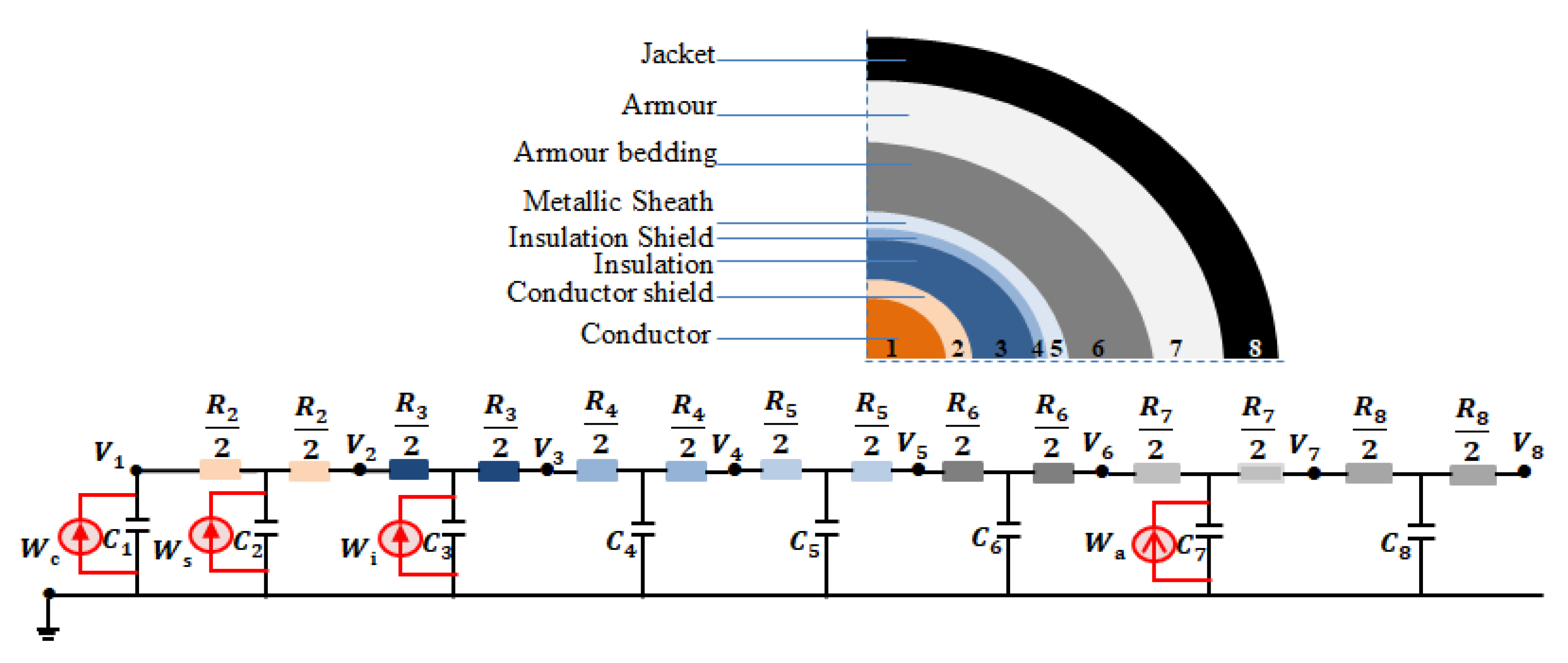
3.1. Power Cable Modelling

The structure of an electrical cable depends on the rated voltage and the type of installation. A single-core cable generic schema is reported in Figure 2, where the main layers are visible. The conductor is generally composed of several copper or aluminium wires to reduce the skin effect. The insulation is typically made of crosslinked polyethylene (XLPE), ethylene propylene rubber (EPR), hard ethylene propylene rubber (HEPR), or polyvinyl chloride (PVC). The insulation is preceded and followed by two semiconducting layers (i.e., the conductor shield and the insulation shield, or internal/external semi-conducting layers), making the electrical field radial inside the insulation, thus improving the power cable performance. The metallic sheath is installed for safety purposes and is usually made of copper or steel tape and fibres. The armour protects the cable from mechanical shock and is usually installed in submarine cables. The jacket protects the cable from mechanical and chemical aggressions.
A very popular approach to implement the thermal cable model is the “thermo-electric equivalent” (also known as “lumped parameters model”), based on the electrothermal analogy summarised in Table 1 [61,62]. All materials are characterised by thermal resistivity and capacity interconnected in series and parallel, considering the cable layout. The current generators represent the equivalent heat sources due to different types of losses (e.g., dielectric losses and Joule losses inside the conductor), which are usually computed according to the Standard IEC 60287-1-1 [51]. To improve the model accuracy, skin-effect, proximity effect, and temperature dependency should be represented since they affect the electrical resistance values, which have an impact on losses [63].
Another way to estimate the electrical resistance of MV cables requires the availability of synchrophasor data given by phasor measurement units (PMUs) [64]. By modelling heat flow with a current in the electric analogy, the different node voltages inherently model the temperatures. Then, the dynamics of the thermal circuit can be represented by using ordinary differential equations [65,66]. The electrothermal approach can be easily extended to model several single-core cables or multicore cables, taking into account the mutual location of the different cores, the presence of further jacketing, and the position of all the cables inside the ducts.
Detailed representations are possible for the equivalent circuit that models the cable in its operational conditions. These representations are formulated for the internal part of the cable and for the outer part that includes the soil and the external ambient. Figure 2 [22] represents the single core of the cable, which has cylindrical symmetry and includes isothermal coaxial layers. The equivalent circuit contains a number of interconnected elements (capacitors, resistors, and generators).
In particular, according to the electrothermal analogy of Table 1, the resistors represent the thermal resistances, the capacitors represent the thermal capacities and are essential to model the thermal transients in real operating conditions. The generators represent the heat sources that originated from different types of losses [67,68]. Between two adjacent layers, the capacitors and resistors can be connected to form “T” or “Π“ double-bipole circuit models with lumped parameters. In Figure 2, all components are represented the “T” circuit model. In some cases, considering the component size and material, it is possible to neglect some resistances (for example, for the shield and the sheath). Looking at the series or parallel connection of resistors and capacitors, it is also possible to reduce the number of corresponding elements that appear in the circuit by summing up any series resistances and any parallel capacitances.

3.2. Computational Methods

Several methods allow the computation of the temperature of the underground cable and of the surrounding soil. Below, the main ones are briefly reported, pointing out their strengths and weaknesses. A general categorisation of the methods is carried out by considering analytic models, finite difference methods, finite element methods, or simplified models and equations.
In analytic models, the analytic solution of the diffusion equation, usually provided in an exponential integral form, allows the computation of the temperature distribution at any point of the soil in homogeneous systems [69,70]. It requires as input the thermal and the electrical resistivity of soil, the distance among the cables and their depth of burial, and, finally, the electrical losses associated with a current flowing through the cables. Scenarios with a single cable or with several conductors laid in a nonsymmetric schema can be easily studied. The main strengths of this method are the ease of implementation, the low computational time, and the absence of convergence criteria. The weakness is that only homogeneous scenarios can be studied [58,70]: this means, for example, that the effect of the presence of different materials in the area surrounding the cables cannot be taken into account. This aspect is a clear simplification considering that the soil in the area under investigation is the result of excavation activity. It can thus have a significant impact on the thermal resistivity of the ground.
The multilayer soil model is another analytical approach, where the underlying idea is to subdivide the area surrounding the cables into several layers that are modelled as an equivalent electrothermal lumped circuit [58,61,71]. The temperature distribution can be easily calculated by solving the circuit. This approach is in line with that of the IEC 60287-1-1 [51] standard and allows a more faithful representation of the temperature distribution [58].
A further analytical model to assess the power cable rating takes into account the non-uniform temperature distribution in the underground space. This temperature distribution is calculated by using the heat-transfer equations with boundary conditions [72]. The classical approach requires concentric layers to model the soil, which, of course, is a hard constraint. A more recent approach overcomes this limitation providing a non-concentric ladder soil model [71].
The finite difference method (FDM) is a numerical method that solves the heat diffusion equation approximating the partial derivatives using finite differences. Since the length of the installation is much greater than the lateral dimensions, the heat diffusion equations are often considered independent of the length coordinate. Within this simplified approach, the solution refers to a plane that is perpendicular to the cable length. The FDM requires a discretisation of the cable and of the surrounding soil, considering cylindrical and rectangular coordinates for the mesh grid [43,73]. One of the inconveniences that may arise is the need to consider a quite large simulation domain around the cables to guarantee that the furthermost points in soil keep their original temperature (i.e., constant temperature isotherms at points far enough from the cables). A variable step discretisation in the mesh building process can be considered so that only the relevant areas can be modelled with a fine mesh, while for the remaining parts, a coarse mesh can be adopted [43].
The finite element method (FEM) is another important numerical method particularly popular in the field [74]. In addition, in this case, the domain of the model (2D or 3D) is meshed. Since the shape of the mesh elements is chosen considering the geometry of the objects, FEM can be considered more flexible than FDM. The mesh generation is often a thorny step in the simulation process, especially when objects characterised by different dimensions coexist. Thereby, simulating a cable with a small cross-section buried in a large piece of land could be complicated.
When the system is represented by using a large number of connected nodes, a crucial issue appears for the creation of a nonregular mesh aimed at reducing the computational burden and improving the effectiveness of the result representation. However, only FEM allows the simulation of complex scenarios, such as those characterised by the presence of multiple circuits [75], ground surface heat [76], cable trench profile [77], concrete and asphalt cover [78,79,80], and mixtures for bedding in a multilayered soil represented in 2D [39]. In steady-state, the FEM minimises a given functional, subject to a set of boundary constraints [81]. Some tools used for two-dimensional (2D) analysis are FEMM [82], FLUX [75], COMSOL with 2D model [83], and ANSYS [55,84]. The numerical model used in the FEM tool developed in [39] contains some nonlinear functions of temperature and is solved by using an approach based on the Newton–Raphson method.
Some FEM software (e.g., COMSOL multiphysics and ANSYS) allows multiphysics simulations for determining the dynamic thermal rating of electrical cables [85,86]. For example, the thermal and the electrical equations of the model are solved together in the simulation process, benefiting the simulation accuracy. In this case, the current distribution in the three-phase current system on the screen and the soil can be calculated considering mutual coupling and skin effects. For submarine cables or overhead lines, the fluid dynamics equations can also be added to model the effects of water and air. Unfortunately, multiphysics analysis usually increases simulation complexity. In fact, considering multiphysics domains often implies multiscaling, which means that the combined physical models have significant differences in space or time scales [87]. For example, in cable current evaluation, an increase in complexity could be due to the different mesh density requirements of the combined physical models: calculation of eddy currents in the thin solid screen requires several layers of finite elements through the thickness of the screen, while a single layer is sufficient for heat-transfer calculation. A multiphysics approach should be carried out, especially when a high simulation accuracy justifies the increment of the simulation complexity. Otherwise, simplifying assumptions can be made without impacting the results [87,88,89].
Recently, three-dimensional (3D) analysis has been used, obtaining results such as the ones reported from the tool FLUX 3D [77], in which the computation time has been quite long even when short cables are considered. Long computation time has also been indicated for the 3D model used in [90] for low-voltage power cables. A high computational burden is needed for obtaining detailed results in 3D FEM analysis, and this is the main limiting factor of FEM. Moreover, FEM cannot provide information to determine the relation between the temperature of the power cable and the various parameters that appear in the thermal circuit model [60].
Simplified models and the corresponding equations have been used for representing various phenomena that determine temperature variations. The use of simplified models has the objective of avoiding the use of FEM and provides reasonable results that can be compared with the FEM solutions. Even though today’s computational power makes it possible to solve highly meshed structures by using FEM, the research on simplified models gives interesting contributions with relatively accurate results in specific cases. In the example reported in [58], soil is represented with multiple layers by using an equivalent circuit that adopts non-uniform discretisation to calculate the results of the thermal transients. By using this model, the results show that the use of five layers can be suitable for providing very close results with respect to the application of FEM. Similarly, in [71], the soil layers are represented by using non-concentric models. In [84], starting from the soil thermal resistance found on the basis of the Standard IEC 60287, the application of some corrective coefficients has been validated with respect to the results found by using 2D FEM. Significant reduction of the computational time with respect to 3D FEM has also been reported in [91] with the use of 3D multiconductor cell analysis, considering a three-core armoured cable with helically wound wires, where, however, no thermal model has been included. The 3D power cable and joint model presented in [92] has provided satisfactory results in comparison with measured values.

4. DCR Impact on Power and Distribution System Operation and Planning

The next subsections describe the integration of DCR in the solution of various operation and planning problems formulated to analyse power and distribution systems. Calculation of the current rating, reliability aspects, and the effects of power cable monitoring are first considered. Then, proposals regarding DCR are categorised according to different time frames. While the real-time methods have been mostly studied with the aim to optimise the asset utilisation, it is possible to apply the concept of dynamic rating, also considering a short-term and long-term operation. In the latter time horizon, planning or design problems are usually addressed. It is worth noting that these methods enable better operation and the upgrading of the sizing procedures for new scenarios.

4.1. Calculation of the Current Rating

Starting from known values of the soil thermal resistivity, the power cables are usually sized by considering the static cable rating (SCR), as recommended by the IEC technical Standard IEC 60287-1-1 [51]. In the SCR, the current-carrying capacity (or ampacity) of the cable is calculated as the continuous current carried by the cable, such as the continuous conductor temperature being equal to the maximum allowable conductor temperature which depends on the insulating material (for example, this temperature is 90 °C for most cables). The SCR is a conservative value since steady-state conditions are assumed to be maintained for the useful life of the cable. Starting from the cable and surrounding thermal model, the Standard IEC 60287-1-1 provides the equations for the current rating with constant load, considering all losses arising in the power cable (Joule losses, dielectric losses, armour and screen losses, etc…). For a buried cable (without soil drying out) or for cables placed in air, the static cable rating I r is:
I r = Δ T W d [ 0.5 R t 1 + n ( R t 2 + R t 3 + R t 4 ) ] R e [ R t 1 + n ( 1 + λ 1 ) R t 2 + n ( 1 + λ 1 + λ 2 ) ( R t 3 + R t 4 ) ]
being:
Δ T : difference between the maximum allowable conductor temperature and the ambient temperature;
W d : dielectric losses for the insulation surrounding the conductor;
R t 1 : thermal resistance between one conductor and the sheath;
R t 2 : thermal resistance between the sheath and the armour;
R t 3 : thermal resistance of the external serving of the cable;
R t 4 : thermal resistance between the cable surface and the surrounding medium;
λ 1 : ratio of losses in the metal sheath to total losses in all conductors;
λ 2 : ratio of losses in the armouring to total losses in all conductors;
R e : electric resistance of the conductor evaluated at the maximum allowable conductor temperature;
n: number of cable conductors.
The Standard IEC 60287-1-1 determines the current rating without exceeding the maximum allowable temperature by applying the Neher–McGrath method [28]. Generalised techniques are introduced in [93] to take into account the soil thermal instability in the calculations based on [28].
The particular problem of deriving the power cable rating equations when the temperature limits are imposed at points different from the power cable conductor external surface is addressed in [70]. The imposition of these limitations is mainly motivated by environmental reasons. The point at which the temperature limit is imposed can be located on the external surface of the power cable, or at a specified location in the surrounding environment. The presence of this additional limit corresponds to impose further constraints to the power cable sizing. This limit has to be also imposed for calculating the solutions under dynamic conditions. The sizing of power cables used to export power from offshore wind farms is addressed in [70] to go beyond the static rating as in the Standard IEC 60287-1-1 and the rating based on the daily cycle as in [51,94].
Another crucial aspect to consider for determining the current rating is the possible uncertainty with which the parameters are known. Different uncertainties could appear, e.g., in the thermophysical soil properties, as well as in the electrical load evolution during time. In the latter case, the uncertainty affects the Joule losses in the power cable [95]. Transient tolerance analysis of cable rating is presented in [96], where interval mathematics is used for the calculations. An online DCR developed for understanding the real-time limits of power-transfer capability, relevant for the user participation in energy and ancillary services markets, is described in [97]. A review on possible ways for increasing the power cable rating is presented in [67].

4.2. Reliability Aspects

For the purpose of reliability analysis, power cables are treated as repairable components. The underground cables are repaired with the construction of joints, in a period of some hours. However, for reliability analysis, the time horizon is based on years, meaning the repair time is relatively short in this respect. In addition, the number of cable failures in one year is generally low; hence, the mean time between failures is much higher than the repair time. This supports the hypothesis that failures are rare events in the lifetime of power cables [98].
With respect to the physical determination of power cable reliability, a supplementary cause for faults is the corrosion stage of the metallic screen shield. This aspect may lead to further degradation of cable reliability. High local electrical fields may cause deterioration of the power cable, especially in the joints when imperfections are introduced during the joint construction [99]. In this case, partial discharges could occur, and the defect could be exacerbated, in particular at high temperatures [100].
A central point in assessing the overall cable reliability is the ability to fast pinpointing the failures on cables. The fast location of cable faults is paramount for ensuring the least possible interruption time for downstream consumers, directly impacting electricity distribution costs. The current practice addresses the fault location with a four-step approach, structured as a gradual development of diagnosis, preconditioning, pre-location, and pinpointing [101].
The position of the hot spots and of the joints are the main information needed for setting up the determination of the cable ageing with the use of proper models. After their construction, the joints are weak points for the power cable structure, because they introduce local electrical and thermal resistances. Moreover, the joints worsen the mechanical performance of the cable, especially when the cables are subject to the repair process after the occurrence of the next failures. For these reasons, the use of a constant value for the failure rate in reliability calculations is insufficient. The outcomes of the service restoration process can be taken into account by using probability distributions of the failure rate that depend on the number of cable joints [102]. Variable representations of the failure rate after the occurrence of repair events, which consider higher failure rates and ageing in reliability analysis, are discussed in [103].
The concerns regarding cable reliability were recognised at the European level and subsequently addressed through interdisciplinary funded research activities. In [104], the ARTEMIS BRITE-EURAM program has been presented, which achieved its main objectives of developing a diagnostic methodology. This methodology has been used to assess both the susceptibility of polymeric cable insulation to electrical ageing and the insulation state at any chosen time to evaluate the remaining lifetime of operating power cables.
The data-driven forecasting approach shown in [105] addresses the remaining life of power cables. The objective is to predict when the cumulative effect of the relevant features that have been chosen to represent the issues under analysis exceeds a specified threshold. In another data-driven method [102], a special emphasis was put on evaluating the reliability of cables with a supplementary aspect of performing a secondary categorisation of cables by considering them repairable or nonrepairable components. The nested algorithm considers the Weibull parametric proportional hazard model (PHM) for analysing and modelling the failure rate of individual cables. The advantage of the PHM method is its independence of additional measurements on the cables, being concentrated on the historical cable parameters and failure data. It has been proved that previous conclusions about the reliability of repairable cables were incorrect due to the inaccurate methods approach. In [106], the reliability methodology that considers the age of cables was expressed in three categories: planning techniques, end-of-life modelling, and replacement planning. Cable ageing indicators are used in [107] by considering different situations, one for normal conditions, and another one in emergency conditions in which there is a higher risk of failures. In short emergency periods, higher cable rating may be considered for the power cables, calculating the cable rating increase through the assessment of the risk of damaging the cable because of worsening its thermal conditions [108].
The existing reporting on ageing influence on cables reliability is scarce, and the scope of reliability modelling is to increase the level of confidence for future failure behaviour. By considering the existence of two failure states, namely repairable and non-repairable failures, the current literature concentrates on repairable failures to the disadvantage of end-of-life failures. The reliability evaluation of power system components takes into consideration the bathtub curve. This curve is composed of three phases, which are characteristic to the early-life (high but decreasing failure rate), useful-life (low and constant failure rate), and end-of-life phase (highly increasing failure rate) [109]. When the useful-life period is considered, the exponential distribution function is used for modelling time to failure and time to repair. Therefore, the time-homogenous Markov process is applied for reliability assessment. By applying the parametric approach, different probabilistic distribution models are tested, and goodness-of-fit tests are used for calculating the parameters from the ‘best fit’ model. The modelling of historical failure data is performed using parametric methods, such log-normal or Weibull, to represent the end-of-life failure over the exponential function because of the lack-of-memory property [110].

4.3. Cable Monitoring

The concerns regarding power cable reliability were recognised at the European level and subsequently addressed through interdisciplinary funded research activities. In the ARTEMIS BRITE-EURAM program, the main innovation is the combined approach of using advanced modelling, theoretical evaluation, and practical testing on real-file cables used in electrical power systems [104]. This approach was a first and led to a fully integrated diagnosis system. For AC electrical power cables, a new model was elaborated for power cable ageing, using advanced (sub) microscopic techniques to monitor and identify relevant ageing markers. This new approach led to new ideas for the future redefinition of installation systems and technologies.
The temperature is the most significant variable for DCR. Temperatures are measured by using thermocouples installed at different locations along the power cable. One can apply several practices to monitor real-time temperature, all of them having advantages and disadvantages. These practices include the placement of optical fibre sensors within the structure of the cable, the location of optical fibres at the external side of the cable, or taking a reference temperature when no current flows in the cable. In all these cases, there is no certainty that the positions where the thermocouples are installed are close to the actual location of the hot spots. Thereby, it is difficult to identify the occurrence of critical conditions at specific points of the cable.
The approach used to obtain the real-time temperature profile for different points along the cable is denoted as distributed temperature sensing (DTS) [111]. DTS consists of placing a number of optical fibre-based sensors in the structure of the power cable [112]. The analysis of the Raman backscatter light in the optical fibre provides the information to draw the temperature profiles. The temperature data are used by supervisory control and data acquisition (SCADA) systems, in which the power cable operation is monitored to provide useful information to identify possible critical points of the power cable or to assist the determination of the effects of the current flowing in the cable.
DTS applications include various challenges [62]. Among them, the cost of the cable increases when the optical fibre is introduced in the cable jacket. Furthermore, the time and cost of making a cable joint increase when jointing the cable has to include the presence of the optical fibre. When the optical fibre is located inside the cable, its structure is helical, meaning the length of the fibre is higher than the length of the cable. An alternative solution is to position the optical fibre in the external part of the cable. In this case, the determination of the soil temperature becomes easier, and the cable repair can be simplified. However, this case has the drawback that the monitored points are far from the points of the conductor or joints, leading to less accurate temperature measurements.
DTS is also applied to extremely high-voltage (EHV) power cables. In this case, the retrofitting of optical fibres for DTS, together with the related monitoring along the overall length of the cable, is not a practical solution [113]. The solution identified is to install optical fibres in a predefined hot-spot area with known characteristics or to locate dedicated probes for the thermal analysis of temperature and properties of the soil in preselected points. This allows confirming the outcomes of specific calculations and verifying that the cable operation does not exceed the design limits. The example shown in [114] presents the results of monitoring an AC submarine cable operated at 52 kV. More indications on how to establish a system for real-time distributed temperature sensing associated with a SCADA system are included in [115]. Further details on DTS requirements, implementations, and applications are presented in [112].
An increase in temperature monitoring effectiveness may be obtained by carrying out a dedicated temperature monitoring to be considered a reference in the conditions in which there is no current flowing in the cable. Starting from this reference, the temperature variations along the power cable when the current flows can be detected and used for assessing the temperature data when the cable is under operation.
The advances in electrical power cable manufacturing are providing cables with optical fibre embedded, which is a significant advance in temperature monitoring by means of optical fibre sensors. This is the best-suited technology for long-range monitoring, with high accuracy (2–3 °C at 30 km with 0.5–1 m resolution), and it relies on Brillouin time domain analysis, as well as Raman distributed temperature sensing [116]. The underlying principle through which these two mechanisms are operating is the extraction of physical parameters from backscattered light, making them extremely accurate at identifying weak points in cables at long distances.
However, the downsize of these measurement techniques is the fact that they are relying upon static frequency scanning, which is not suitable to follow the dynamic nature of cable operation [117]. There is an array of solutions for this issue, among which are the use of multimode fibre used for simultaneous measurements [118], sweep-free and slope-assisted configurations [119], and optical unipolar pulse coding schemes [120].
The evolution in cable monitoring is an inherent request of both utilities and customers to improve the energy supply service, enhancing it for the needs of the smart grid. These needs range from constant variability of energy flows following market signals [121] to increase power capacity of cables for solving feeding adequacy-related issues [122].
In the smart grid, the system operator must use hardware- and software-monitoring means that ensure the ability to accurately identify the weak points subject to failure for predictive reliability. This reduces operating costs, with consequent reduction of energy bills at end-customers.
The integration of underground cables into the smart grid generates a large database, resulting from continuous and comprehensive monitoring [123]. The resulting database is embedded in a multipurpose-built computing environment, used for automatic control of energy assets [124]. The database is analysed by means of machine-learning techniques [125], in order to continuously feed a human (or automated) grid operator with deep knowledge and situational awareness regarding cable operation, condition, and ability to respond to a sudden increase in power flows.

4.4. Real Time DCR

Real-time monitoring of the cable loading current and the ambient conditions allows determining the cable real-time ratings by imposing the maximum permissible conductor temperature according to the insulating material covering the conductor. The calculations of the real-time ratings aim at improving the utilisation of cables, also lowering security margins. Cable loading currents and ambient conditions are available when monitored (this is the case when the lines are equipped with DTS) or can be accurately estimated when not monitored. Proper estimation techniques have to be established [126].
Real-time cable rating systems have been proposed to perform calculations of steady-state and emergency cable ratings in real-time in [127]. While the objective is to maximise the utilisation of existing cables maintaining the same level of reliability, the calculation of ratings is based on the IEC technical standards [51]. The moisture content of the cable surroundings is considered in [61], where the thermal resistivity and specific heat of the cable surroundings are calculated in function of the actual moisture content and the cooling effect during rainy weather is taken into account. The focus of the contents in [128] is the estimation of the soil thermal parameters considering the measurements of DTS (cable loading current and temperature of the cable surface) over several days; an optimisation problem is combined with the application of FEM.
To improve the real-time thermal rating of power cables, more accurate and sometimes approximate models for the transient temperature calculation are needed. Significant are the models proposed in [58] and [129], aimed at accurately calculating the transient temperature to enrich a DTS system used for real-time DCR. In particular, a representation of the soil is proposed [58], and the presence of other cables in proximity has been considered and modelled [129]. An improved thermal model proposed for the transient temperature calculation in [66] is based on the approximate solution for the Van Wormer coefficient, treated as a time-varying variable. To better represent the soil thermal response, a non-concentric soil layer model is proposed in [71]. Borbuev et al. [126] address the unbalanced loading of the cables and propose an adequate thermal model of cable and soil to handle unbalances. The models are implemented to evaluate the real-time cable ratings and exploit a thermal map of a distribution network.

4.5. Short-Term DCR

Reference [130] addresses the forecasting of the DCR on intraday and day-ahead time-scales with rigorous modelling of the cable–soil thermal–hydraulic dynamics; this is an important point because the thermal transfer between the cable and the soil (and, as a consequence, the conductor temperature) is influenced by the dynamic characteristics of the cable surrounding (i.e., temperature of the soil where the cable is buried, thermal resistivity, and thermal diffusivity of the soil) is affected by the dynamic soil characteristics. In [130], there is the proposal of two methods applied to DCR for intraday and day-ahead forecasting. The first method is a physical–statistical method, while the second method is data-driven. In particular, with respect to the first method, forecasts of the soil temperature at the upper layer, precipitation, and cable current are obtained by applying a support vector regression-based method. First, the environmental conditions are forecast, and then, the dynamic characteristics of the soil are assessed through the thermal–hydraulic model of the soil. Finally, the thermal model of a buried cable proposed by IEC standards for transients provides the forecasting of the DCR at the target hour, in such a way the conductor temperature results less than the allowable value. With respect to the second method, the environmental conditions are forecast based on available measurements of the environmental conditions and on available weather forecasts of precipitation and soil temperature at the upper layer, and the dynamic characteristics of soil are determined by applying the thermal–hydraulic model. Then, the historical DCR is determined by applying the thermal model of a buried cable for transient conditions. Finally, the regression model on historical DCR values allows forecasting the DCR at the target hour.
The references [131,132] consider the export cables for offshore wind farms, and temperature risk assessment is carried out with a probabilistic approach. When a cable exporting the generation of offshore wind farms is considered, the uncertainty of cable current is linked to the uncertainty in the wind power generation. If the cable loading is greater than the cable rating and the temperature is less than the maximum admissible value, power curtailments are not necessary. If the thermal risk hours are estimated in advance, power curtailments can be limited with the obvious advantage of maximising wind energy transportation.
The study reported in [131] proposes the estimation of the difference between the maximum allowable temperature and the cable temperature 6, 12, and 24 h ahead; in this way, it is possible to maximize the power flowing from the offshore wind farm to the landfall. In particular, power curtailments are decided based on a risk index. In the probabilistic procedure outlined in [131], at the first step, the export cable current is estimated in the hours ahead (6, 12, or 24 h) by considering the historical data of wind speed and the power curve. The temperature of the conductor is, then, determined by applying a finite difference analysis of the cable, and the risk of exceeding the maximum allowable temperature is calculated. In [132], the estimation of cable temperatures 6 h ahead allows the evaluation of the probability of the overheating of the cable.

4.6. Long-Term DCR

Planning or designing of cable systems can be addressed considering the concepts of dynamic cable rating. For these problems, cable loading currents and ambient conditions have to be assigned over a long period of time.
As described in Section 4.1, the static cable rating is determined by assuming a constant load and considering the losses such as ohmic losses, dielectric losses, armour, screen and sheath losses, etc. To select the cable section, the static cable rating is compared with the cable operating current. In particular conditions, however, if this sizing method is applied, under-utilised components can be included in the system when the currents are characterized by a high variability. As a consequence, when the worst case is assumed, the static current rating is a conservative value, and the capacity of the cable can be underestimated. An example is the export cable connecting wind farms (already considered in Section 4.5) characterised by “low capacity factors and high-power production variability” [133].
Reduced nominal values in assigned conditions may result when diverse sizing methods are considered. In fact, with respect to traditional thermal sizing, it is likely to obtain an increase in the current rating and a decrease in the cable cross-section [134].
Let us consider the sizing of the offshore export cables. The variability of cable loading can be taken into account, and the procedure for the cyclic ratings for cables, suggested by IEC standards [95,135], can be applied. In particular, the mentioned IEC standards propose a cyclic rating factor, and the formulas are provided for a single cable and for groups of equally loaded identical cables; the cyclic rating factor is, then, multiplied by the maximum allowable current during the daily cycle. The sizing is aimed, also in this case, at meeting the constraint on the maximum allowable temperature. The typical feature of the daily cycle affects the value of the cyclic rating factor; on the contrary, the magnitudes of the currents do not influence the factor [95,135]. In [136], the export cable of offshore wind farms are sized by applying a procedure based on IEC 60853-2 [95], and the equivalent cyclic load profile is obtained from historical wind speed measurements. The approach presented in [137], instead, is based on a dynamic cyclic load profile, consisting, in the worst case, of equivalent stepwise load profiles. When the daily load variations cannot be used, the dynamic rating equation is based on a yearly load cycle that includes long durations of the peak load, followed by long durations of no load.
The export cable of offshore wind farms is taken into consideration also in [138] that proposes an iterative dynamic cable rating method applied to three-core XLPE submarine cables. In the iterative method, an important point is the thermal cable analysis that follows the indications of IEC 60853-2 [95] and includes a thermal ladder network to determine the transient temperature response. The dynamic cable rating is carried out with an iterative procedure: at first, the section of the cable is selected, and the cable current and the parameters of the thermal ladder network are assigned; then, the conductor temperature is determined. The iterative procedure ends when the chosen cable has a conductor temperature less than the maximum allowable temperature.
Reference [133] provides an extensive review of the sizing methods for export cables to connect offshore wind farms to the landfall, including the methods based on DCR.

5. Final Remarks

In this paper, the conceptual aspects and developments concerning the dynamic cable rating have been addressed by reviewing various literature contributions. These contributions have recalled the historical evolution of methods and formulations, also indicating the developments in progress. The classical conceptualisation based on the representation of heat-transfer phenomena has evolved to incorporate more detailed aspects for non-uniform soil, moisture migration, and dry zones. More refined mathematical models have been progressively defined to study hot spots and the ways to mitigate the related issues. The power cable modelling has been developed mainly for enabling implementations in FEM solvers. For these solvers, the computation time is one of the limiting factors that makes the transition from 2D to 3D models particularly challenging.
Moreover, computation time limits the creation of time-dependent models. It is possible to simulate the power cable behaviour considering the variation in operating and external conditions. Even though the thermal phenomena have a relatively slow evolution in time with respect to the electrical phenomena, the time horizon considered for simulations has to be sufficiently long to track the thermal evolution of the power cable operation. One of the main objectives of tracking the thermal and electrical phenomena is to predict the occurrence of failures in the power cable in such a way as to enable preventive maintenance. An interesting line of research is the development of analytical ladder soil models, which seem to be able to provide results comparable with FEM in a shorter time. Currently, the implemented models are mainly 2D and consider only constant currents. A comprehensive framework platform to simulate more complex scenarios is one of the next goals in the field. Extended cable monitoring is required to provide more data for model validation. However, being impossible to monitor all the points in the cable, the choice of the points to be monitored is crucial, together with establishing a sound simulation model to represent the overall cable structure with the surrounding environment. Other tools based on risk analysis, used to estimate the maximum allowable temperature, assist the decision maker in setting up strategies to reduce the curtailment of intermittent generation from renewable energy sources. Data analysis tools with the integration of physical and statistical models are available and have to be improved to enhance the accuracy of DCR forecasting at different time scales. The aspects reported above indicate the vast interest and timeliness of the DCR research in progress.
Further research in the field of DCR can be addressed in several directions. A common theme deserving further deepening is the accurate modelling of single cables as well multiple cable systems; the inclusion of the rigorous representation of the surrounding (including moisture migration phenomena) improves the temperature estimation.
Since multiple sources of uncertainty are recognised among the data, more studies and new methodologies to calculate the DCR accounting for uncertainty will represent a step forward to improve the process of decision making and/or the real-time applications.
Reliability may have a decisive influence on the future development of smart grids, which are foreseen to have far lower interruption time for the users and at a similar energy price with traditional power systems. In this context, the underground cables must be adequately monitored and included in a far-reaching smart grid forecasting environment. This environment must take into account a dynamic database of characteristics, such as wind speed, solar irradiance, air and ground temperature, load variation, battery state of charge, load-shedding algorithms agreed with the customer, and elasticity economically incentivised by the system operator or a local energy market. More accurate DCR forecasting methodologies, if developed, will allow the prediction of the thermal rating in advance reliably; in this research area, probabilistic forecasting of DCR can be elaborated.
An important aspect for future cable rating is the introduction of more electric vehicle charging stations, which will be built, for the sake of saving costs, over the existent power systems infrastructure. This situation may lead to a further strain of existing cables for increased power flows. This will have a significant influence on the deployment of DCR methodologies aimed at reducing risks, maintaining high degrees of service reliability.
New perspectives are also opened by extreme weather phenomena (like heat waves and cold waves), whose probability of occurrence has increased in recent years. As known, these events could affect power systems operation, and proper methodologies for DCR can be applied to minimise their impact and reduce the system vulnerability.
Finally, the application of dynamic rating concepts to further power system equipment should be considered, and it will open new prospects in the planning and operation of electric power systems. In particular, the application of these methodologies, in the frame of modern power systems, will facilitate the integration of renewable sources such as wind or solar generations and avoid or reduce inefficient curtailment actions.

Author Contributions

Conceptualisation, D.E., P.C., A.R., R.F.P. and G.C.S.; methodology, D.E., P.C., A.R., R.F.P. and G.C.S.; formal analysis, D.E., P.C., A.R., R.F.P. and G.C.S.; investigation, D.E., P.C., A.R., R.F.P. and G.C.S.; writing—original draft preparation, D.E., P.C., A.R., R.F.P. and G.C.S.; writing—review and editing, D.E., P.C., A.R., R.F.P. and G.C.S.; visualisation, D.E., P.C., A.R., R.F.P. and G.C.S.; supervision, D.E., P.C., A.R., R.F.P. and G.C.S.; project administration, D.E., R.F.P. and G.C.S., funding acquisition, D.E., P.C., A.R., R.F.P. and G.C.S. All authors have read and agreed to the published version of the manuscript.

Funding

This research received no external funding.

Institutional Review Board Statement

Not applicable.

Informed Consent Statement

Not applicable.

Data Availability Statement

Not applicable.

Acknowledgments

D.E., R.F.P. and G.C.S. acknowledge that this article has been prepared in the framework of a collaboration referring to the European Union’s Horizon 2020 research and innovation programme established under grant agreement No. 774407.

Conflicts of Interest

The authors declare no conflict of interest.

Nomenclature

DLRDynamic Line Rating
DTRDynamic Thermal Rating
DTSDistributed Temperature Sensing
EPREthylene Propylene Rubber
FDMFinite Difference Method
FEMFinite Element Method
EHVExtremely High Voltage
EVElectric Vehicles
HEPRHard Ethylene Propylene Rubber
IECInternational Electrotechnical Commission
MVMedium Voltage
PHMProportional Hazard Model
PMUPhasor Measurement Unit
PVCPolyvinyl Chloride
RMSRoot Mean Square
SCADASupervisory Control And Data Acquisition
SCRStatic Cable Rating
XLPECrosslinked Polyethylene

References

  1. IRENA. Innovation Landscape Brief: Dynamic Line Rating; International Renewable Energy Agency: Abu Dhabi, United Arab Emirates, 2020. [Google Scholar]
  2. Coletta, G.; Vaccaro, A.; Villacci, D. A review of the enabling methodologies for PMUs-based dynamic thermal rating of power transmission lines. Electr. Power Syst. Res. 2017, 152, 257–270. [Google Scholar] [CrossRef]
  3. Morozovska, K.; Naim, W.; Viafora, N.; Shayesteh, E.; Hilber, P. A framework for application of dynamic line rating to aluminium conductor steel reinforced cables based on mechanical strength and durability. Int. J. Electr. Power Energy Syst. 2020, 116, 1–11. [Google Scholar] [CrossRef]
  4. Dabbaghjamanesh, M.; Kavousi-Fard, A.; Mehraeen, S. Effective scheduling of reconfigurable microgrids with dynamic thermal line rating. IEEE Trans. Ind. Electron. 2019, 66, 1552–1564. [Google Scholar] [CrossRef]
  5. Coletta, G.; Laso, A.; Jónsdóttir, G.M.; Manana, M.; Villacci, D.; Vaccaro, A.; Milano, F. On-Line Control of DERs to Enhance the Dynamic Thermal Rating of Transmission Lines. IEEE Trans. Sustain. Energy 2020, 11, 2836–2844. [Google Scholar] [CrossRef]
  6. Safdarian, A.; Degefa, M.Z.; Fotuhi-Firuzabad, M.; Lehtonen, M. Benefits of Real-Time Monitoring to Distribution Systems: Dynamic Thermal Rating. IEEE Trans. Smart Grid 2015, 6, 2023–2031. [Google Scholar] [CrossRef]
  7. Karimi, S.; Musilek, P.; Knight, A.M. Dynamic thermal rating of transmission lines: A review. Renew. Sust. Energy Rev. 2018, 91, 600–612. [Google Scholar] [CrossRef]
  8. Rocha, O.D.A.; Morozovska, K.; Laneryd, T.; Ivarsson, O.; Ahlrot, C.; Hilber, P. Dynamic rating assists cost-effective expansion of wind farms by utilising the hidden capacity of transformers. Int. J. Electr. Power Energy Syst. 2020, 123, 106188. [Google Scholar] [CrossRef]
  9. Daminov, I.; Prokhorov, A.; Caire, R.; Alvarez-Herault, M.C. Assessment of dynamic transformer rating, considering current and temperature limitations. Int. J. Electr. Power Energy Syst. 2021, 129, 106886. [Google Scholar] [CrossRef]
  10. Bracale, A.; Carpinelli, G.; de Falco, P. Probabilistic risk-based management of distribution transformers by dynamic transformer rating. Int. J. Electr. Power Energy Syst. 2019, 113, 229–243. [Google Scholar] [CrossRef]
  11. Liu, S.; Kopsidas, K. Risk-Based Underground Cable Circuit Ratings for Flexible Wind Power Integration. IEEE Trans. Power Deliv. 2021, 36, 145–155. [Google Scholar] [CrossRef]
  12. Ocłoń, P.; Cisek, P.; Matysiak, M. Analysis of an application possibility of geopolymer materials as thermal backfill for underground power cable system. Clean Technol. Environ. Policy 2020, 23, 869–878. [Google Scholar] [CrossRef]
  13. Chatzipanagiotou, P.; Chatziathanasiou, V.; de Mey, G.; Więcek, B. Influence of soil humidity on the thermal impedance, time constant and structure function of underground cables: A laboratory experiment. Appl. Therm. Eng. 2017, 113, 1444–1451. [Google Scholar] [CrossRef]
  14. Alwan, S.H.; Jasni, J.; Ab Kadir, M.Z.A.; Aziz, N. Factors Affecting Current Ratings for Underground and Air Cable. Int. J. Energy Power Eng. 2016, 10, 1422–1428. [Google Scholar]
  15. Anders, G. Rating of Electric Power Cables in Unfavorable Thermal Environment; IEEE Press: Piscataway, NJ, USA, 2005. [Google Scholar]
  16. Czapp, S.; Ratkowski, F. Effect of soil moisture on current-carrying capacity of low-voltage power cables. Przegląd Elektrotechniczny 2019, 95, 154–159. [Google Scholar] [CrossRef]
  17. Gouda, O.E.; Abdel-Aziz, A.M.; Refale, R.A.; Matter, Z. Experimental study for drying-out of soil around underground power cables. Eng. Sci. 1992, 9, 23–40. [Google Scholar]
  18. Bates, C.; Malmedal, K.; Cain, D. Cable Ampacity Calculations: A Comparison of Methods. IEEE Trans. Ind. Appl. 2016, 52, 112–118. [Google Scholar] [CrossRef]
  19. De Lieto Vollaro, R.; Fontana, L.; Vallati, A. Experimental study of thermal field deriving from an underground electrical power cable buried in non-homogeneous soils. Appl. Therm. Eng. 2014, 62, 390–397. [Google Scholar] [CrossRef]
  20. Al–Saud, M.S.; El-Kady, M.A.; Findlay, R.D. A new approach to underground cable performance assessment. Electr. Power Syst. Res. 2008, 78, 907–918. [Google Scholar] [CrossRef]
  21. Enescu, D.; Colella, P.; Russo, A. Thermal Assessment of Power Cables and Impacts on Cable Current Rating: An Overview. Energies 2020, 13, 5319. [Google Scholar] [CrossRef]
  22. Enescu, D.; Russo, A.; Porumb, R.; Seritan, G. Dynamic Thermal Rating of Electric Cables: A Conceptual Overview. In Proceedings of the 55th International Universities Power Engineering Conference (UPEC), Torino, Italy, 1–4 September 2020. [Google Scholar]
  23. Erdinç, F.G.; Erdinç, O.; Yumurtacı, R.; Catalão, J.P.S. A Comprehensive Overview of Dynamic Line Rating Combined with Other Flexibility Options from an Operational Point of View. Energies 2020, 13, 6563. [Google Scholar] [CrossRef]
  24. Carslaw, H.C.; Jaeger, J.C. Conduction of Heat in Solids; Oxford University Press: Oxford, UK, 1986. [Google Scholar]
  25. Rees, S.W.; Adjali, M.H.; Zhou, Z.; Davies, M.; Thomas, H.R. Ground heat transfer effects on the thermal performance of earth-contact structures. Renew. Sust. Energy Rev. 2000, 4, 213–265. [Google Scholar] [CrossRef]
  26. Bouddour, A.; Auriault, J.L.; Mhamdi-Alaoui, M. Heat and mass transfer in wet porous media in presence of evaporation-condensation. Int. J. Heat Mass Transf. 1988, 41, 2263–2277. [Google Scholar] [CrossRef]
  27. International Electrotechnical Commission. IEC 60287-1-1: Calculations of the Continuous Current Rating of Cables (100% Load Factor); International Electrotechnical Commission: Geneva, Switzerland, 1982. [Google Scholar]
  28. Neher, J.H.; McGrath, M.H. The calculation of the temperature rise and load capability of cable systems. Trans. Am. Inst. Elect. Eng. Power Appl. Syst. Part III 1957, 76, 752–772. [Google Scholar] [CrossRef]
  29. Salata, F.; Nardecchia, F.; Gugliermetti, F.; Vollaro, A. How thermal conductivity of excavation materials affects the behavior of underground power cables. Appl. Therm. Eng. 2016, 100, 528–537. [Google Scholar] [CrossRef]
  30. Hamed, S.; Behrooz, V. A probabilistic approach for optimal power cable ampacity computation by considering uncertainty of parameters and economic constraints. Int. J. Electr. Power Energy Syst. Mar. 2019, 106, 432–443. [Google Scholar]
  31. Peters-Lidard, C.D.; Blackburn, E.; Liang, X.; Wood, E.F. The effect of soil thermal conductivity parameterisation on surface energy fluxes and temperatures. J. Atmos. Sci. 1998, 55, 1209–1224. [Google Scholar] [CrossRef]
  32. Abu-Hamdeh, N.H. Thermal properties of soils as affected by density and water content. Biosyst. Eng. 2003, 86, 97–102. [Google Scholar] [CrossRef]
  33. Van den Brink, G.J.; Hoogendoorn, C.J. Ground water flow heat losses for seasonal heat storage in the soil. Sol. Energy 1983, 30, 367–371. [Google Scholar] [CrossRef]
  34. De Vries, D. Thermal properties of soils. Phys. Plant. Environ. 1963, 1, 57–109. [Google Scholar]
  35. Farouki, O.T. Thermal properties of soils. Series Rock Soil Mech. 1986, 11, 1–136. [Google Scholar]
  36. Campbell, G.S.; Jungbauer, J., Jr.; Bidlake, W.; Hungerford, R. Predicting the effect of temperature on soil thermal conductivity. Soil. Sci. 1994, 158, 307–313. [Google Scholar] [CrossRef]
  37. Kroener, E.; Vallati, A.; Bittelli, M. Numerical simulation of coupled heat, liquid water and water vapor in soils for heat dissipation of underground electrical power cables. Appl. Therm. Eng. 2014, 70, 510–523. [Google Scholar] [CrossRef]
  38. Ghanbarian, B.; Daigle, H. Thermal conductivity in porous media: Percolation-based effective-medium approximation. Water Resour. Res. 2016, 52, 295–314. [Google Scholar] [CrossRef] [Green Version]
  39. Ocłoń, P.; Cisek, P.; Pilarczyk, M.; Taler, D. Numerical simulation of heat dissipation processes in underground power cable system situated in thermal backfill and buried in a multilayered soil. Energy Convers. Manag. 2015, 951, 352–370. [Google Scholar] [CrossRef]
  40. Gouda, O.E.; El Dein, A.Z.; Amer, M.G. Effect of the formation of the dry zone around underground power cables on their rating. IEEE Trans. Power Deliv. 2011, 26, 972–978. [Google Scholar] [CrossRef]
  41. Anders, G.J.; Radhakrishna, H.S. Power cable thermal analysis with consideration of heat and moisture transfer in the soil. IEEE Trans. Power Deliv. 1988, 3, 1280–1288. [Google Scholar] [CrossRef]
  42. Lu, H.; de León, F.; Soni, D.N.; Wang, W. Two-Zone Geological Soil Moisture Migration Model for Cable Thermal Rating. IEEE Trans. Power Deliv. 2018, 33, 3196–3204. [Google Scholar] [CrossRef]
  43. Garrido, C.; Otero, A.F.; Cidrás, J. Theoretical model to calculate steady-state and transient ampacity and temperature in buried cables. IEEE Trans. Power Deliv. 2003, 18, 667–678. [Google Scholar] [CrossRef]
  44. De León, F.; Anders, G.J. Effects of backfilling on cable ampacity analysed with the finite element method. IEEE Trans. Power Del. 2008, 23, 537–543. [Google Scholar] [CrossRef]
  45. Ocłoń, P.; Bittelli, M.; Cisek, P.; Kroener, E.; Pilarczyk, M.; Taler, D.; Rao, R.V.; Vallati, A. The performance analysis of a new thermal backfill material for underground power cable system. Appl. Therm. Eng. 2016, 108, 233–250. [Google Scholar] [CrossRef]
  46. Kim, Y.S.; Kim, J.; Cho, D.S. Implementation of optimised backfill materials for underground electric power cables. J. Porous Media 2014, 17, 831–840. [Google Scholar] [CrossRef]
  47. Brakelmann, H.; Anders, G.J.; Cherukupalli, S. Underground cable hot spot. IEEE Trans. Power Deliv. 2020, 35, 592–599. [Google Scholar] [CrossRef]
  48. Tobin, B.; Zadehgol, H.; Ho, K.; Welsh, G.; Prestrud, J. A water cooling system to improve ampacity in underground urban distribution cables. In Proceedings of the IEEE/PES Transmission and Distribution Conference and Exhibition, Dallas, TX, USA, 21–24 May 2006; pp. 432–437. [Google Scholar]
  49. Klimenta, D.; Tasi, D.; Jevti, M. The use of hydronic asphalt pavements as an alternative method of eliminating hot spots of underground power cables. Appl. Therm. Eng. 2020, 168, 114818. [Google Scholar] [CrossRef]
  50. Klimenta, D.; Tasić, D.; Jevtić, M. An alternative method of increasing the transmission performance of a conventional 110 kV cable line. J. Energy Technol. 2019, 12, 1–10. [Google Scholar]
  51. International Electrotechnical Commission. IEC 60287-1-1: Electric Cables—Calculation of the Current Rating—Part 1-1: Current Rating Equations (100% Load Factor) and Calculation of Losses—General; International Electrotechnical Commission: Geneva, Switzerland, 2006. [Google Scholar]
  52. Hruška, M.; Clauser, C.; De Doncker, R.W. Influence of dry ambient conditions on performance of underground medium-voltage DC cables. Appl. Therm. Eng. 2019, 149, 1419–1426. [Google Scholar] [CrossRef]
  53. Philip, J.R.; de Vries, D.A. Moisture movements in porous materials under temperature gradients. Trans. Am. Geophys. Union 1957, 38, 222–232. [Google Scholar] [CrossRef]
  54. Groeneveld, G.J.; Snijders, A.L.; Koopmans, G.; Vermeer, J. Improved method to calculate the critical conditions for drying out sandy soils around power cables. IEEE Proc. 1984, 131, 42–53. [Google Scholar] [CrossRef]
  55. Bustamante, S.; Mínguez, R.; Arroyo, A.; Manana, M.; Laso, A.; Castro, P.; Martinez, R. Thermal behaviour of medium-voltage underground cables under high-load operating conditions. Appl. Therm. Eng. 2019, 156, 444–452. [Google Scholar] [CrossRef]
  56. Ocłoń, P.; Pobędza, J.; Walczak, P.; Cisek, P.; Vallati, A. Experimental Validation of a Heat Transfer Model in Underground Power Cable Systems. Energies 2020, 13, 1747. [Google Scholar] [CrossRef] [Green Version]
  57. International Electrotechnical Commission. IEC 60287-3-1/2 Electric Cables e Calculation of the Current Rating e Sections on Operating Conditions; International Electrotechnical Commission: Geneva, Switzerland, 1999. [Google Scholar]
  58. Diaz–Aguiló, M.; de León, F.; Jazebi, S.; Terracciano, M. Ladder–Type Soil Model for Dynamic Thermal Rating of Underground Power Cable. IEEE Power Energy Technol. Syst. J. 2014, 1, 21–30. [Google Scholar] [CrossRef]
  59. Kovač, N.; Sarajčev, I.; Poljak, D. Nonlinear-coupled electric-thermal modeling of underground cable systems. IEEE Trans. Power Deliv. 2006, 21, 4–14. [Google Scholar] [CrossRef]
  60. Kocar, I.; Ertas, A. Thermal Analysis for Determination of Current Carrying Capacity of PE and XLPE Insulated Power Cables Using Finite Element Method. In Proceedings of the 12th IEEE Mediterranean Electrotechnical Conference (Melecon 2004), Dubrovnik, Croatia, 12–15 May 2004. [Google Scholar]
  61. Olsen, R.S.; Anders, G.J.; Holboell, J.; Gudmundsdottir, U.S. Modelling of dynamic transmission cable temperature considering soil-specific heat thermal resistivity, and precipitation. IEEE Trans. Power Deliv. 2013, 28, 1909–1917. [Google Scholar] [CrossRef] [Green Version]
  62. Bascom, E.C., III; Clairmont, B. Considerations for advanced temperature monitoring of underground power cables. In Proceedings of the IEEE PES T&D Conference and Exposition, Chicago, IL, USA, 14–17 April 2014. [Google Scholar]
  63. Sugihara, H.; Funaki, T. Analysis on Temperature Dependency of Effective AC Conductor Resistance of Underground Cables for Dynamic Line Ratings. In Proceedings of the Smart Grids, IEEE 21st International Conference on High Performance Computing and Communications—IEEE 17th International Conference on Smart City—IEEE 5th International Conference on Data Science and Systems (HPCC/SmartCity/DSS), Zhangjiajie, China, 10–12 August 2019. [Google Scholar]
  64. Singh, R.S.; Cobben, S.; Gibescu, M.; van den Brom, H.; Colangelo, D.; Rietveld, G. Medium Voltage Line Parameter Estimation Using Synchrophasor Data: A Step Towards Dynamic Line Rating. In Proceedings of the IEEE Power & Energy Society General Meeting (PESGM), Portland, OR, USA, 5–10 August 2018. [Google Scholar]
  65. Bontempi, G.; Vaccaro, A.; Villacci, D. Power cables’ thermal protection by interval simulation of imprecise dynamical systems. IEEE Proc. Gener. Transm. Distrib. 2004, 151, 673–680. [Google Scholar] [CrossRef]
  66. Wang, P.; Ma, H.; Liu, G.; Han, Z.Z.; Guo, D.M.; Xu, T.; Kang, L.Y. Dynamic Thermal Analysis of High-Voltage Power Cable Insulation for Cable Dynamic Thermal Rating. IEEE Access 2019, 7, 56095–56106. [Google Scholar] [CrossRef]
  67. Benato, R.; Colla, L.; Dambone Sessa, S.; Marelli, M. Review of high current rating insulated cable solutions. Electr. Power Syst. Res. 2016, 133, 36–41. [Google Scholar] [CrossRef]
  68. Arias Velásquez, R.M.; Mejía Lara, J.V. New methodology for design and failure analysis of underground transmission lines. Eng. Fail. Anal. 2020, 115, 104604. [Google Scholar] [CrossRef]
  69. Anders, G.J. Rating of Electric Power Cables; McGraw–Hill: New York, NY, USA, 1997. [Google Scholar]
  70. Anders, G.J.; Brakelmann, H. Rating of Underground Power Cables with Boundary Temperature Restrictions. IEEE Trans. Power Deliv. 2018, 33, 1895–1902. [Google Scholar] [CrossRef]
  71. Lux, J.; Czerniuk, T.; Olschewski, M.; Hill, W. Non-Concentric Ladder Soil Model for Dynamic Rating of Buried Power Cables. IEEE Trans. Power Deliv. 2021, 36, 235–243. [Google Scholar] [CrossRef]
  72. Maximov, S.; Venegas, V.; Guardado, J.L.; Moreno, E.L.; López, R. Analysis of underground cable ampacity considering non–uniform soil temperature distributions. Electr. Power Syst. Res. 2016, 132, 22–29. [Google Scholar] [CrossRef]
  73. Haskew, T.A.; Carwile, R.F.; Grigsby, L.L. An algorithm for steady-state thermal analysis of electrical cables with radiation by reduced Newton-Raphson techniques. IEEE Trans. Power Deliv. 1994, 9, 526–533. [Google Scholar] [CrossRef]
  74. Nahman, J.; Tanaskovic, M. Determination of the current carrying capacity of cables using the finite element method. Electr. Power Syst. Res. 2002, 61, 109–117. [Google Scholar] [CrossRef]
  75. Desmet, J.; Putman, D.; Vanalme, G.; Belmans, R.; Vandommelent, D. Thermal analysis of parallel underground energy cables. In Proceedings of the CIRED 2005—18th International Conference and Exhibition on Electricity Distribution, Turin, Italy, 6–9 June 2005; pp. 1–4. [Google Scholar]
  76. Nahman, J.; Tanaskovic, M.; Tanaskovic, M. Calculation of the loading capacity of high voltage cables laid in close proximity to heat pipelines using iterative finite-element method. Int. J. Electr. Power Energy Syst. 2018, 103, 310–316. [Google Scholar] [CrossRef]
  77. Benato, R.; Dambone Sessa, S.; Forzan, M.; Marelli, M.; Pietribiasi, D. Core laying pitch–long 3D finite element model of an AC three–core armoured submarine cable with a length of 3 meter. Electr. Power Syst. Res. 2017, 150, 137–143. [Google Scholar] [CrossRef]
  78. Hwang, C.C.; Chang, J.J.; Chen, H.Y. Calculation of ampacities for cables in trays using finite elements. Electr. Power Syst. Res. 2000, 54, 75–81. [Google Scholar] [CrossRef]
  79. Vaucheret, P.; Hartlein, R.A.; Black, W.Z. Ampacity Derating Factors for Cables Buried in Short Segments of Conduit. IEEE Trans. Power Deliv. 2005, 20, 560–565. [Google Scholar] [CrossRef]
  80. Demoulias, C.; Labridis, D.P.; Dokopoulos, P.S.; Gouramanis, K. Influence of metallic trays on the ac resistance and ampacity of low-voltage cables under non-sinusoidal currents. Electr. Power Syst. Res. 2008, 78, 883–896. [Google Scholar] [CrossRef]
  81. Al–Saud, M.S. Assessment of thermal performance of underground current carrying conductors. IET Gener. Transm. Distrib. 2011, 5, 630–639. [Google Scholar] [CrossRef]
  82. Jenkins, L.; Fahmi, N.; Yang, J. Application of dynamic asset rating on the UK LV and 11 kV underground power distribution network. In Proceedings of the 52nd International Universities Power Engineering Conference (UPEC), Heraklion, Greece, 28–31 August 2017; pp. 1–6. [Google Scholar]
  83. Snajdr, J.; Lucak, J.; Vostracky, Z.; Kozeny, J. Dynamic rating of supply cables of a stabilising furnace. In Proceedings of the 2014 15th International Scientific Conference on Electric Power Engineering (EPE), Brno-Bystrc, Czech Republic, 12–14 May 2014; pp. 507–510. [Google Scholar]
  84. Salata, F.; Nardecchia, F.; de Lieto Vollaro, A.; Gugliermetti, F. Underground electric cables a correct evaluation of the soil thermal resistance. Appl. Therm. Eng. 2015, 785, 268–277. [Google Scholar] [CrossRef]
  85. COMSOL Multiphysics. Comsol Multi-Physics User Guide (Version 4.3 a); COMSOL: Burlington, MA, USA, 2012. [Google Scholar]
  86. Ansys. Guide, ANSYS FLUENT User. Release 14.0; ANSYS. Inc.: Canonsburg, PA, USA, 2011. [Google Scholar]
  87. Korovkin, N.; Greshnyakov, G.; Dubitsky, S. Multiphysics approach to the boundary problems of power engineering and their application to the analysis of load-carrying capacity of power cable line. In Proceedings of the Electric Power Quality and Supply Reliability Conference (PQ), Rakvere, Estonia, 11–13 June 2014; pp. 341–346. [Google Scholar]
  88. Dubitsky, S.; Greshnyakov, G.; Korovkin, N. Refinement of underground power cable ampacity by multiphysics FEA simulation. Int. J. Energy 2015, 9, 12–19. [Google Scholar]
  89. Dubitsky, S.; Greshnyakov, G.; Korovkin, N. Comparison of finite element analysis to IEC-60287 for predicting underground cable ampacity. In Proceedings of the IEEE International Energy Conference (ENERGYCON), Leuven, Belgium, 4–8 April 2016; pp. 1–6. [Google Scholar]
  90. Delgado, F.; Renedo, C.J.; Ortiz, A.; Fernández, I.; Santisteban, A. 3D thermal model and experimental validation of a low voltage three-phase busduct. Appl. Therm. Eng. 2017, 110, 1643–1652. [Google Scholar] [CrossRef] [Green Version]
  91. Benato, R.; Dambone Sessa, S. A New Multiconductor Cell Three–Dimension Matrix–Based Analysis Applied to a Three–Core Armoured Cable. IEEE Trans. Power Deliv. 2018, 33, 1636–1646. [Google Scholar] [CrossRef]
  92. Bragatto, T.; Cresta, M.; Gatta, F.M.; Geri, A.; Maccioni, M.; Paulucci, M. A 3-D nonlinear thermal circuit model of underground MV power cables and their joints. Electr. Power Syst. Res. 2019, 73, 112–121. [Google Scholar] [CrossRef]
  93. Bates, C.; Malmedal, K.; Cain, D. How to Include Soil Thermal Instability in Underground Cable Ampacity Calculations. In Proceedings of the IEEE Industry Applications Society Annual Meeting, Portland, OR, USA, 2–6 October 2016. [Google Scholar]
  94. International Electrotechnical Commission. IEC 60853-2: Calculation of the Cyclic and Emergency Current Rating of Cables. Part 2: Cyclic Rating of Cables Greater Than 18/30 (36) kV and Emergency Ratings for Cables of All Voltages; International Electrotechnical Commission: Geneva, Switzerland, 1989. [Google Scholar]
  95. Foty, M.S.; Anders, G.J.; Croall, S.C. Cable environment analysis and the probabilistic approach to cable rating. IEEE Trans. Power Deliv. 1990, 5, 1628–1633. [Google Scholar] [CrossRef]
  96. Villacci, D.; Vaccaro, A. Transient tolerance analysis of power cables thermal dynamic by interval mathematic. Electr. Power Syst. Res. 2007, 77, 308–314. [Google Scholar] [CrossRef]
  97. Huang, S.H.; Lee, W.J.; Kuo, M.T. An Online Dynamic Cable Rating System for an Industrial Power Plant in the Restructured Electric Market. IEEE Trans. Ind. Appl. 2007, 43, 1449–1458. [Google Scholar] [CrossRef]
  98. Carpaneto, E.; Chicco, G.; Porumb, R.; Roggero, E. Probabilistic representation of the distribution system restoration times. In Proceedings of the CIRED 2005–18th International Conference and Exhibition on Electricity Distribution, Turin, Italy, 6–9 June 2005. [Google Scholar]
  99. Calcara, L.; D’Orazio, L.; Della Corte, M.; Di Filippo., G.; Pastore, A.; Ricci, D.; Pompili, M. Faults Evaluation of MV Underground Cable Joints. In Proceedings of the International Annual Conference (AEIT), Florence, Italy, 18–20 September 2019; pp. 1–6. [Google Scholar]
  100. Calcara, L.; Sangiovanni, S.; Pompili, M. MV underground cables: Effects of soil thermal resistivity on anomalous working temperatures. In Proceedings of the International Annual Conference (AEIT), Cagliari, Italy, 20–22 September 2017; pp. 1–5. [Google Scholar]
  101. Laughton, M.A.; Warne, D.F. Electrical Engineer’s Reference Book, 16th ed.; Elsevier: Amsterdam, The Netherlands, 2002; pp. 31/35–31/40. [Google Scholar]
  102. Nemati, H.M.; Sant’Anna, A.; Nowaczyk, S.; Jürgensen, J.H.; Hilber, P. Reliability evaluation of power cables considering the restoration characteristic. Int. J. Electr. Power Energy Syst. 2019, 105, 622–631. [Google Scholar] [CrossRef]
  103. Gill, Y. Development of an electrical cable replacement simulation model to aid with the management of aging underground electric cables. IEEE Electr. Insul. Mag. 2011, 27, 31–37. [Google Scholar] [CrossRef]
  104. Garros, B. Ageing and reliability testing and monitoring of power cables: Diagnosis for insulation systems: The ARTEMIS program. IEEE Electr. Insul. Mag. 1999, 15, 10–12. [Google Scholar] [CrossRef]
  105. Liu, S.; Wang, Y.; Tian, F. Prognosis of Underground Cable via Online Data-Driven Method with Field Data. IEEE Trans. Ind. Electron. 2015, 62, 786–7794. [Google Scholar] [CrossRef]
  106. Buhari, M. Reliability Assessment of Ageing Distribution Cable for Replacement in Smart Distribution Systems. Ph.D. Thesis, Faculty of Science and Engineering, The University of Manchester, Manchester, UK, June 2016. [Google Scholar]
  107. Kopsidas, K.; Liu, S. Power Network Reliability Framework for Integrating Cable Design and Ageing. IEEE Trans. Power Syst. 2018, 33, 1521–1532. [Google Scholar] [CrossRef]
  108. Clements, D.; Mancarella, P.; Ash, R. Application of time-limited ratings to underground cables to enable life extension of network assets. In Proceedings of the International Conference on Probabilistic Methods Applied to Power Systems (PMAPS), Beijing, China, 16–20 October 2016. [Google Scholar]
  109. Allan, R.N.; Billinton, R. Reliability Evaluation of Power Systems; Springer: Berlin/Heidelberg, Germany, 1996. [Google Scholar]
  110. Billinton, R.; Allan, R.N. Reliability Evaluation of Engineering Systems: Concepts and Techniques; Springer: Berlin/Heidelberg, Germany, 1992. [Google Scholar]
  111. Singh, K. Cable monitoring solution—Predict with certainty. In Proceedings of the 12th IET International Conference on Developments in Power System Protection (DPSP), Copenhagen, Denmark, 31 March–3 April 2014. [Google Scholar]
  112. Cherukupalli, S.; Anders, G.J. Distributed Fiber Sensing and Dynamic Rating of Power Cables; Wiley: Hoboken, NJ, USA, 2020. [Google Scholar]
  113. Marazzato, H.; Barber, K.; Jansen, M.; Barnewall, G. Cable Condition Monitoring of Improve Reliability. In Proceedings of the TechCon Asia-Pacific, OLEX, Sydney, Australia; 2004. Available online: https://www.nexans.co.nz/NewZealand/2012/22_1.04.2004%20-%20Cable%20Condition%20Monitoring.pdf (accessed on 29 April 2021).
  114. Cherukupalli, S.; Adapa, R.; Bascom, E.C., III. Implementation of Quasi-Real-Time Rating Software to Monitor 525 kV Cable Systems. IEEE Trans. Power Deliv. 2019, 34, 1309–1316. [Google Scholar] [CrossRef]
  115. Cherukupalli, S.; Anders, G.J. How Can Temperature Data Be Used to Forecast Circuit Ratings? In Distributed Fiber Optic Sensing and Dynamic Rating of Power Cables; Cherukupalli, S., Anders, G.J., Eds.; Wiley: Hoboken, NJ, USA, 2020; Chapter 9; pp. 129–165. [Google Scholar]
  116. Muanenda, Y.; Oton, C.J.; di Pasquale, F. Application of Raman and Brillouin Scattering Phenomena in Distributed Optical Fiber Sensing. Front. Phys. 2019, 7, 155. [Google Scholar] [CrossRef]
  117. Chen, D.; Liu, Q.; Fan, X.; He, Z. Distributed fiber-optic acoustic sensor with enhanced response bandwidth and high signal-to-noise ratio. J. Lightw. Technol. 2017, 35, 2037–2043. [Google Scholar] [CrossRef]
  118. Wang, D.; Cheng, B.; Jin, B.; Wang, Y.; Zhang, M.; Liu, X.; Bai, Q. Remote simultaneous measurement of liquid temperature and refractive index using fiber-optic spontaneous Raman scattering. IEEE Sens. J. 2019, 19, 10513–10518. [Google Scholar] [CrossRef]
  119. Zhou, D.; Dong, Y.; Wang, B.; Jiang, T.; Ba, D.; Xu, P.; Zhang, H.; Lu, Z.; Li, H. Slope-assisted BOTDA based on vector SBS and frequency-agile technique for wide-strain-range dynamic measurements. Opt. Express 2017, 25, 1889–1902. [Google Scholar] [CrossRef] [Green Version]
  120. Yang, Z.; Li, Z.; Zaslawski, S.; Thévenaz, L.; Soto, M.A. Design rules for optimizing unipolar coded Brillouin optical time-domain analyzers. Opt. Express 2018, 26, 16505–16523. [Google Scholar] [CrossRef]
  121. Manusov, V.Z.; Khasanzoda, N.; Atabaeva, L.S. Two-Way Energy Flow Optimization Based on Smart Grid Concept. In Proceedings of the 2018 International Conference on Industrial Engineering, Applications and Manufacturing (ICIEAM), Moscow, Russia, 15–18 May 2018. [Google Scholar]
  122. Shekhar, A.; Kontos, E.; Ramírez-Elizondo, L.; Rodrigo-Mor, A.; Bauer, P. Grid capacity and efficiency enhancement by operating medium voltage AC cables as DC links with modular multilevel converters. Int. J. Electr. Power Energy Syst. 2017, 93, 479–493. [Google Scholar] [CrossRef]
  123. Jianming, Q.; Jizhen, L.; Yuebin, H.; Jianhua, Z. Use of real-time/historical database in Smart Grid. In Proceedings of the 2011 International Conference on Electric Information and Control Engineering, Wuhan, China, 15–17 April 2011. [Google Scholar]
  124. Cartes, D.; Chow, J.H.; McCaugherty, D.; Widergren, S. (Eds.) Smart Grid Research: Computing—IEEE Smart Grid Vision for Computing: 2030 and Beyond; IEEE Publishing: New York, NY, USA, 2003. [Google Scholar]
  125. Huo, Y.; Prasad, G.; Lampe, L.; Leung, C.M.V. Smart-Grid Monitoring: Enhanced Machine Learning for Cable Diagnostics. In Proceedings of the 2019 IEEE International Symposium on Power Line Communications and its Applications (ISPLC), Prague, Czech Republic, 3–5 April 2019. [Google Scholar]
  126. Borbuev, A.; Wang, W.; Lu, H.; Jazebi, S.; de Leon, F. Investment Deferral of Feeder Upgrades Revealed by System-Wide Unbalanced Dynamic Rating: Harvesting the Hidden Capacity of Distribution Systems Discovered by Thermal Map Technology. IEEE Trans. Power Deliv. 2020, in press. [Google Scholar] [CrossRef]
  127. Anders, G.J.; Napieralski, A.; Zubert, M.; Orlikowski, M. Advanced modeling techniques for dynamic feeder rating systems. IEEE Trans. Ind. Appl. 2003, 39, 619–626. [Google Scholar] [CrossRef]
  128. Li, H.; Tan, K.; Su, Q. Assessment of Underground Cable Ratings Based on Distributed Temperature Sensing. IEEE Trans. Power Deliv. 2006, 21, 1763–1769. [Google Scholar] [CrossRef]
  129. Diaz–Aguiló, M.; de León, F. Introducing Mutual Heating Effects in the Ladder-Type Soil Model for the Dynamic Thermal Rating of Underground Cables. IEEE Trans. Power Deliv. 2015, 30, 1958–1964. [Google Scholar] [CrossRef]
  130. Bracale, A.; Caramia, P.; de Falco, P.; Michiorri, A.; Russo, A. Day-Ahead and Intraday Forecasts of the Dynamic Line Rating for Buried Cables. IEEE Access 2019, 7, 4709–4725. [Google Scholar] [CrossRef]
  131. Hernandez Colin, M.A.; Pilgrim, J.A. Offshore Cable Optimisation by Probabilistic Thermal Risk Estimation. In Proceedings of the IEEE International Conference on Probabilistic Methods Applied to Power Systems (PMAPS), Boise, ID, USA, 23–28 June 2018; pp. 1–6. [Google Scholar]
  132. Hernandez Colin, M.A.; Pilgrim, J.A. Cable Thermal Risk Estimation for Overplanted Wind Farms. IEEE Trans. Power Deliv. 2020, 35, 609–617. [Google Scholar] [CrossRef]
  133. Pérez-Rúa, J.A.; Cutululis, N.A. Electrical Cable Optimization in Offshore Wind Farms—A Review. IEEE Access 2019, 7, 85796–85811. [Google Scholar] [CrossRef]
  134. Colla, L.; Marelli, M. Dynamic Rating of Submarine Cables. Application to Offshore Windfarms. In Proceedings of the European Wind Energy Association (EWEA) Offshore Conference, Frankfurt, Germany, 19–21 November 2013. [Google Scholar]
  135. International Electrotechnical Commission. IEC 60853-1: Calculation of the Cyclic and Emergency Current Rating of Cables—Part 1: Cyclic Rating Factor for Cables Up to and Including 18/30 (36) kV; International Electrotechnical Commission: Geneva, Switzerland, 1985. [Google Scholar]
  136. Catmull, S.; Chippendale, R.D.; Pilgrim, J.A.; Hutton, G.; Cangy, P. Cyclic Load Profiles for Offshore Wind Farm Cable Rating. IEEE Trans. Power Deliv. 2016, 31, 1242–1250. [Google Scholar] [CrossRef]
  137. CIGRE Working Group B1.40. Offshore Generation Cable Connections; Technical Brochure n. 610; e-Cigre: Paris, France, 2015. [Google Scholar]
  138. Nielsen, T.V.M.; Jakobsen, S.; Savaghebi, M. Dynamic Rating of Three–Core XLPE Submarine Cables for Offshore Wind Farms. Appl. Sci. 2019, 9, 800. [Google Scholar] [CrossRef] [Green Version]
Figure 1. Single cable in backfill material and trench cross-section.
Energies 14 02591 g001
Figure 2. Equivalent electrical model from electrothermal analogy for a single-core cable, considering the representation of the parameters with the “T” model.
Energies 14 02591 g002
Table 1. Electrothermal analogy.
Thermal QuantityUnitsElectrical QuantityUnits
Temperature TKElectric potential VV
Absolute zero0 KGround potential0 V
Heat flow rate Q ˙ WElectric current IA
Thermal conductivity kW/(m·K)Electric conductivity γ1/(Ω·m)
Thermal capacity CtJ/KCapacitance CeF
Thermal resistance RtK/WElectrical resistance ReΩ
Publisher’s Note: MDPI stays neutral with regard to jurisdictional claims in published maps and institutional affiliations.

