Humidity in Power Converters of Wind Turbines—Field Conditions and Their Relation with Failures

Abstract

Power converters in wind turbines exhibit frequent failures, the causes of which have remained unexplained for years. Field-experience based research has revealed that power- and thermal-cycling induced fatigue effects in power electronics do not contribute significantly to the field failures observed. Instead, clear seasonal failure patterns point to environmental influences, in particular to humidity, as a critical stressor and likely driver of converter failure. In addition to the electrical operating conditions, it is therefore important to also identify and characterize the climatic conditions that power converters in wind turbines are exposed to, both as a contribution to root-cause analysis and as a basis for the derivation of suitable test procedures for reliability qualification of components and systems. This paper summarizes the results of field-measurement campaigns in 31 wind turbines of seven different manufacturers spread over three continents. The temperature and humidity conditions inside the converter cabinets are characterized and related to the environmental conditions of the turbines and to their operation. The cabinet-internal climate is found to be subject to pronounced seasonal variations. In addition to the site-specific ambient climatic conditions and the operation of the turbines, the converter cooling concept is identified to significantly influence the climatic conditions inside the power cabinets.

1. Introduction

Since the early days of their utilization, power converters have been among the most frequently failing components of wind turbines, as major reliability studies in the past decade, e.g., [1,2,3], have confirmed. Their failures cause considerable revenue losses related to maintenance and downtime. Increasing their reliability is therefore an important contribution to further reducing the levelized cost (LCOE) of wind energy. A prerequisite for the development of effective measures, however, is an understanding of the failure modes prevailing in the field and of the underlying causes and mechanisms. For many years, research on the reliability of power electronics in wind turbines was strongly focused on power- and thermal-cycling induced fatigue effects on the chip and packaging level, which were assumed to be the dominant failure cause also in the power converters of wind turbines (cf. [4] for a variety of examples that are based on this postulation). However, comprehensive field-experience based research of the Fraunhofer Institute for Wind Energy Systems IWES, Germany, using failure data from thousands of wind turbines (WT) around the world in combination with post-mortem analysis of field-returned converter components revealed that the above fatigue effects are not among the prevailing causes of the converter failures observed in today’s wind turbines [4,5,6]. Instead, the observed strong seasonal clustering of failures points to climatic influences, in particular to humidity, as a relevant stressor and likely cause of converter failure [4,6]. Wind-power specific results of other research groups confirm the relevance of humidity in the context of converter failure: based on data from an older WT fleet, Tavner et al. [7] revealed a clear correlation between WT failures and weather conditions, with temperature and humidity having an even more significant effect than wind speed. In more recent studies based on younger WT fleets, Su and Hu [8] reported a strong clustering of electrical-system failures in wind turbines in China during months with warm and humid ambient conditions. Reder [9] found that the power converters failed mainly at low wind speeds, mild monthly mean temperatures and high ambient relative humidity.

In parallel to the increasing awareness of climatic influences as a critical driver for converter failures in wind turbines, a shift in focus towards environmental effects on reliability and particularly humidity issues is observable also in other fields of application of power electronic converters. This is indicated by publications such as [10,11,12], but also by the numerous contributions and strong industrial interest in a recent workshop of the European Center for Power Electronics (ECPE) on this subject [13]. In general, the trend towards miniaturization and higher component density in electronics increases their susceptibility to humidity, as pointed out in [14,15]. This is due to (1) higher packaging densities coming along with reduced distances of components and conducting tracks that facilitate a bridging, e.g., by water droplets or growing filaments; (2) higher electrical field strengths being a key driver for migration and corrosion effects; and (3) lower heat generation and with that reduced self-heating.

A result of the growing awareness of the relevance of environmental impact on power electronics reliability is a strongly increasing interest in the real climatic conditions experienced by these components in the different applications. One example are traction converters, for which the ongoing EU-funded PINTA projects in the Shift2Rail Joint Undertaking cover field measurements to better understand the environmental requirements in the railway application [16].

For power converters in wind power applications, we recognized the importance of understanding not only the electrical but also the climatic operating conditions in WT already within the first field-experience based study [17]. For this reason, Fraunhofer IWES has carried out numerous field-measurement campaigns in cooperation with WT operators since 2012, the results of which are the main subject of the present paper. Single climatic time series collected in this way were published earlier by the authors in [5,17,18,19]. In addition, exemplary climatic data measured in the converter of a WT were published by Brunko et al. in [20]. Compared with these previously published examples, the present paper takes a substantial step forward, both with respect to the amount and variety of the datasets and sites evaluated and to the depth of analysis.

The aim of this paper is

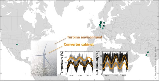
• to characterize the climatic conditions in converter cabinets of WT based on humidity and temperature data collected in turbines on three different continents,
• to relate these to the ambient climatic conditions and the WT operating conditions,
• to identify potential dependencies on the converter cooling concept and position and
• to shed light on the question why different seasonal failure patterns are observed in air-cooled and liquid-cooled converters of WT [4].

The paper is structured as follows: Section 2 introduces the instrumentation used for the climatic field measurements and describes the evaluated datasets and sites. Section 3 presents and discusses a variety of results derived from the measurement data. Finally, Section 4 summarizes the main conclusions of the present paper.

2. Materials and Methods

The climatic measurement data presented and evaluated in this paper have been collected since 2012 in a wide variety of onshore and offshore wind turbines at sites on three different continents (see Figure 1). The measurements have covered wind turbines with a nominal power in the range of 1.5–6.2 MW, including turbines both with fully and partially rated converter, with converter positions in the nacelle and in the tower base as well as turbines with air-cooled and liquid-cooled converters. The measured datasets cover periods ranging from some weeks to several years. The instrumentation used for measuring the climatic conditions inside (and in single cases outside) the wind turbines and supplementary data relevant for the analysis are described in the following.

2.1. Temperature and Humidity Measurement Campaigns

In most cases, the climatic conditions have been recorded by means of small battery-supplied loggers of type EasyLog EL-USB-2 by Lascar Electronics shown in Figure 2. These log the air temperature, relative humidity (RH) as well as the resulting dew-point temperature. Due to the limited storage capacity of the loggers, sampling intervals of 15 or 30 min have been used in order to allow long measurement periods. The loggers are specified for use in a temperature range of −35–80 °C and at 0–100% RH and have a precision of 0.5 °C and 0.5%, respectively. While the typical accuracy is 0.3 °C and 2% RH, the specified maximum errors are ±1.2 °C and ±5% RH at very low or very high temperature and humidity conditions [21]. The number of loggers installed per WT has varied and increased through the years: During the first measurement campaigns, loggers were placed solely inside the power cabinets, to measure the climatic conditions in the cabinet air near the power electronics. In later campaigns, additional loggers have been installed outside of the power cabinet, in the converter-control cabinet and, in single cases, at the outside of the turbine.

As an important and valuable complement, many of the project partners involved in the measurement campaigns have provided Fraunhofer IWES with operating data (10 min-aggregated data from the Supervisory Control and Data Acquisition (SCADA) system) from the wind turbines and periods of interest.

In addition to the logger-based measurements described above, comprehensive data from own climatic field-measurement campaigns in three WT in India and Texas were provided by a project partner and included in the analysis. In these campaigns, the turbines were equipped with PT100 temperature sensors by EPHY MESS at various points inside and outside the converter cabinets. An EE16-type sensor by E + E Elektronik measuring temperature and relative humidity (accuracy of ±0.5 °C and ±3% RH at 20 °C [22]) was placed inside the converter cabinet in two cases and outside of the cabinet in the third turbine, respectively. A Bachmann programmable logic controller (PLC) was used for data acquisition in intervals of 1 min, which included also electrical operating data of the WT received from the converter control system.

2.2. Supplementary Site-Specific Environmental Data (ERA5)

The climatic conditions in a converter cabinet are a result of the WT-ambient conditions, its design and its operation. In order to understand their dependency on the different influences, it is of crucial importance to have information also on the environmental conditions around the turbines. In the present work, we use the publicly available ERA5 reanalysis data for this purpose. ERA5 provides a large number of hourly estimates of relevant atmospheric and oceanographic variables based on global modal data. The dataset covers the earth on a grid of approximately 30 km × 30 km. For detailed information on the ERA5 reanalysis data, please refer to [23].

The variables of the ERA5 dataset used in the present study are the temperature and the dew-point temperature, both 2 m above the ground. Their time series consist of instantaneous values with a temporal resolution of 1 h. Combining temperature and dew-point temperature, the absolute and relative humidity are calculated.

2.3. Methods of Analysis

An important step preceding any evaluation of field data is its thorough pre-processing. In case of the measurement and operating data from different sources used in the present work, this has covered the transformation into a consistent format and structure as well as a cleansing from implausible data points.

Conversions between different measures of humidity (i.e., calculation of absolute humidity from temperature and relative humidity in case of the measurement data and calculation of relative and absolute humidity from temperature and dew point in case of ERA5 data, respectively) have been performed in agreement with those underlying the conversions used in model simulations for the generation of the ERA5 reanalysis, assuming saturation over water and using Teten’s formula with parameters according to Buck [24] for calculating saturation water vapor pressure (cf. documentation in [25,26]):

$$e_{sat}\left(T\right)=k_1·\exp \left(k_2·\frac{T-T_0}{T-k_3}\right)$$

(1)

Herein, T denotes the absolute temperature (in Kelvin) and the parameter values are k₁ = 611.21 Pa, k₂ = 17.502, k₃ = 32.19 K and T₀ = 273.16 K [24]. The relative humidity RH is defined as the quotient of vapor pressure e and saturation vapor pressure e_sat and therefore depends on the temperature T and the dew-point temperature T_dp according to:

$$RH=100\%·\frac{e}{e_{sat}}=100\%·\frac{e_{sat}\left(T_{dp}\right)}{e_{sat}\left(T\right)}$$

(2)

The absolute humidity AH as the mass of vapor (moisture) m_w per volume of air V can be calculated from vapor pressure and absolute temperature using the equation

$$AH=\frac{m_w}{V}=\frac{e}{R_w·T}=\frac{e_{sat}\left(T_{dp}\right)}{R_w·T}$$

(3)

with R_w = 461.51 J/(kg K) denoting the specific gas constant for water vapor.

A variety of methods are subsequently applied for the evaluation of the measured data:

• The starting point is the analysis of visualized measured temperature and humidity time series along with the ambient climatic conditions in the wind farm (site-specific ERA5 data) and with the WT operating point (i.e., active power fed to the grid normalized with the rated power of the WT). Note that due to the direct transferability of dew-point temperature into absolute humidity and vice versa, we limit the presentation in this paper to only one of these quantities. In the presentation and discussion of results, it should be understood that statements on one of these quantities apply in the same way to the second one.
• The temperature and humidity conditions inside the converter cabinets are characterized by means of two-dimensional histograms showing the range of values and distributions of these signals.
• Based on the periodicities observed in the data, sinusoidal functions are fitted to the temperature and humidity time series by means of nonlinear regression, similarly to the procedure presented in [27] for the case of ambient climatic data:

  $$f\left(t\right) =A_0+A_1·\cos \left(2\pi ·\frac{t-A_2}{365 d}\right)$$

  (4)
  A simple comparison of some aggregated descriptive statistics (e.g., measures of location or dispersion) of the temperature and humidity would lead to misleading results due to the pronounced seasonal variations in climatic conditions and the different lengths of measurement periods, which typically deviate from full-year periods. In this situation, the fitting of sinusoidal functions to the WT-internal and WT-external climatic time series is a suitable method to allow a systematic comparative analysis across different sites, WT types and measurement periods.
• Scatterplots of the estimated parameters of the sinusoidal regression functions (e.g., the constant terms, the amplitudes and phase shifts) are used to reveal similarities and differences of the WT under analysis and identify how design factors such as the converter position in the WT or the cooling concept of the converter influence the climatic conditions in the converter cabinets.

For the calculation of failure rates shown in the present work, only faults requiring on-site repair and the consumption of spare parts or other material are considered as failure events. The average failure rate of a component is calculated according to the equation (see also, e.g., [4]):

$$f=\frac{{{\displaystyle \sum }}_{i=1}^I{N}_i}{{{\displaystyle \sum }}_{i=1}^I{X}_i·T_i}=\frac{N}{T}$$

(5)

In this equation, N_i describes the number of failure events of the component in the time interval i. X_i denotes the total number of turbines evaluated in this time interval, and T_i describes the duration of the time interval. Consequently, the average failure rate equals the quotient of the overall number N of failure events of the component of interest and the total number of evaluated wind-turbine operating years T. Note that the latter must include the operating time of both the failed and the non-failed turbines.

As a simple measure of correlation, the linear correlation coefficient (also: Pearson’s correlation coefficient) will be used at various points in this paper. It quantifies the strength of a linear relationship between two variables x and y and is estimated from a series of n pairs of data, denoted x_i and y_i, and their sample mean values, denoted x_m and y_m, using:

$$r_{xy}=\frac{{{\displaystyle \sum }}_{i=1}^n\left(x_i-x_m\right)\left(y_i-y_m\right)}{\sqrt{{{\displaystyle \sum }}_{i=1}^n{\left(x_i-x_m\right)}^2{{\displaystyle \sum }}_{i=1}^n{\left(y_i-y_m\right)}^2}}$$

(6)

A second quantity of interest in the context of correlation analysis is the p-value for testing the null hypothesis of no correlation against the alternative that there is a correlation. For further information on the linear correlation coefficient or the corresponding p-value see, e.g., [28].

All data processing and analysis underlying the present work has been performed in MATLAB, version 2018b.

3. Results and Discussion

An extensive amount of data has been collected in the measurement campaigns described in Section 2 and through tapping the ERA5 database for the corresponding site-specific ambient conditions. Not all information gathered can be included in this study. Therefore, we seek a balance between an in-depth presentation of selected cases and analyses covering the measurement data from all investigated sites and WT types in the following. The starting point, however, is dedicated to an example of the seasonal converter-failure patterns forming the background and motivation of the field measurement campaigns of climatic conditions in WT converters.

3.1. Seasonal Converter Failure Patterns and Relation with Ambient Conditions

In close collaboration with project partners, Fraunhofer IWES has been able to collect and evaluate an increasing amount of converter-specific failure data through the past years. Today, the failure dataset covers more than 10,000 WT spread over Europe, Asia, Australia as well as North and South America. The exploratory statistical analysis of these data has revealed seasonal failure patterns in different regions, which has suggested a comparison with the local wind and climatic conditions. Figure 3 shows the most pronounced of these seasonal patterns, which has been observed in a WT fleet with liquid-cooled converters in India (cf. also [4,6]): It indicates that during the particularly humid months of June to September, the average failure rates of the core converter components (also denoted ‘phase-module’ components, incl. the insulated-gate bipolar transistor (IGBT) modules, their driver boards as well as the DC-link capacitors and busbars) rise to multiples of the previous months and decrease again notably towards the end of the year.

In contrast to the previous publications [4,6], in which this pattern could be compared only to averaged information from single Indian weather stations, we now compare these measurements specifically to the meteorological ERA5 reanalysis data for the wind farms and time periods of interests (see the lower subplots of Figure 3). The monthly averaged time series make clear how diverse not only the wind but also the ambient climatic conditions can be within a single country. As a simple quantitative measure of correlation between the monthly average failure rates and the ambient conditions, we provide the linear correlation coefficient r for each of the environmental quantities. It is calculated based on the monthly average values across all wind farms of interest (included as grey markers in Figure 3). The r values indicate a particularly strong correlation of the phase-module failure rates with the ambient measures of humidity, both with the relative humidity (r = 0.86) and the dew-point temperature (r = 0.68). The corresponding p-values are 0.0003 and 0.0146. Using a significance level of α = 0.05, the p-values confirm that these correlations are statistically significant.

Figure 4 provides a deepened analysis on the relation of phase-module failures and the ambient climatic conditions of the turbines. It evaluates the temperature and humidity conditions at the time of failure and seeks to identify which conditions increase the risk of failure. As the exact timestamp of failure (i.e., not only the date but also the time of day of failure) must be known for this type of analysis, only turbines for which SCADA data are also available can be included. The analysis underlying Figure 4 is therefore limited to a subset of the data underlying Figure 3 that covers 243 WT operating years. To illustrate the analysis procedure, Figure 4 consists of three subfigures: The overall range of ambient temperature and dew-point temperature is split into several bins. Depending on the conditions at the time of failure determined from the site-specific ERA5 data, each failure event is assigned to one of these bins. Figure 4a shows the resulting absolute number of failures in each of the bins. While no failures in the investigated fleet have been recorded at dew-point temperature values below 0 °C, the by far highest number of failures occurred at temperatures above 25 °C and dew-point temperatures above 15 °C. However, as Figure 4b makes clear, these are also the conditions at which the turbines of the evaluated Indian fleet are operating most of the time. In order to come to a meaningful analysis, it is necessary to take into consideration also the distribution of operating time over the different bins. Figure 4c is therefore derived by dividing for each bin the number of failures by the accumulated WT operating years falling into this bin, which results in the presentation of an average failure rate for each bin that can be interpreted. Would the failure events emerge independently of the ambient climatic conditions, the failure rates in all bins would be expected to be of the same magnitude. As Figure 4c shows, this is not the case. Instead a clear increase in the failure rates (and with that the risk of failure) is found with increasing level of ambient temperature and humidity. In addition to the comparison with monthly averaged conditions in Figure 3, this provides further evidence that the climatic conditions play an important role in the emergence of WT converter failures.

While a comparison of failure rates and WT-ambient conditions as in Figure 3 and Figure 4 can provide indications about influences that promote failure, it is necessary to understand the climatic conditions inside the WT and particularly inside their converter cabinets to further clarify the prevailing drivers and mechanisms of failure.

3.2. Climatic Conditions in Converter Cabinets of Wind Turbines

Among the 31 WT from which turbine-internal measurement data were collected, three are selected for an in-depth presentation:

• an onshore WT with an air-cooled converter in the tower base located in the federal state of Thuringia in Germany,
• an offshore WT in the German North Sea with a liquid-cooled converter in the nacelle, and
• an onshore WT located in India with a liquid-cooled converter in the tower base.

The three turbines are serial models of different types and manufacturers. A similarity across the three WT is that they use doubly fed induction generators (DFIG) with partially rated converters. In these, the converter rating is typically approx. 25% of the WT’s rated power.

3.2.1. Example 1: Onshore WT in Germany with Air-Cooled Converter in the Tower Base

The first dataset stems from a WT located in the German Federal State of Thuringia, i.e., onshore at a distance of approximately 300 km from the sea. With a rated power in the range of 1.5 MW, it is an older-type turbine that has been installed in large numbers particularly in the first decade of this century. The power converter of this WT (also referred to as WT1 in the following) is air-cooled and located in the tower base.

Figure 5 shows the temperature and humidity time series measured inside and outside the converter cabinet as well as the WT-ambient climatic conditions according to the WT’s SCADA data and the site-specific ERA5 data. (Note that the SCADA dataset of this WT contains no humidity signals.) The last subplot complements the time series of climatic conditions with information about the corresponding operating points of the turbine: It shows the WT’s 10-min-averaged active power fed to the electric power grid normalized with the rated power of the turbine.

While Figure 5 visualizes the data from the whole measurement period of approx. ten months and is thus suitable to provide the overall picture and reveal seasonal variations, it is too coarse to identify details. For the same WT1, Figure 6 therefore provides segments of the time series limited to several days in summer and in winter, respectively. Note that all time stamps used and provided in this paper are in UTC (Coordinated Universal Time).

In a first step, we focus on a comparison of the conditions inside and outside the WT: As the uppermost subplot shows, there are notable differences between the temperature levels inside the converter cabinet, outside the cabinet inside the tower and outside the WT. With only rare exceptions, the highest temperature level is found inside the converter cabinet. This is expectable particularly during operation of the turbine, due to the losses generated in the electrically loaded converter. In this context, it is important to note that the power flow through the partial converter in a DFIG system is not proportional to the overall power the WT feeds into the grid: It undergoes a reversal of direction and with that a minimum of the absolute value in the point of synchronism of the DFIG (see, e.g., [29] for further details). The power flow through the converter takes on maximum values when the WT operates at full load. It is therefore plausible that the highest differences between cabinet-internal and WT-external temperatures are encountered during high part-load or full-load operation of the turbine (cf. the uppermost and the lowest subplot in Figure 6, see, e.g., 7th January in comparison with 9 January 2017). Correlation analysis reveals a strong linear correlation (r = 0.90) of the cabinet-internal temperature with the ERA5 WT-ambient temperature and a lower (r = 0.22), but likewise statistically significant correlation (p < 0.0001) between the cabinet-internal temperature and the WT active power. An interesting detail related to the temperature time series is that values below 0 °C can be observed inside this WT. These low values are encountered not only inside the tower but also within the converter cabinet (see 6 January 2017 in Figure 6). Surprising enough, a turbine start-up takes place in this condition in the early morning hours of 7 January 2017 without any notable preheating of the converter.

In case of the relative humidity, the levels inside and outside the WT differ even stronger than the temperature levels, as the RH plots in Figure 5 and Figure 6 make clear. There is only a moderate linear correlation between the cabinet-internal and the WT-external RH (r = 0.54). A very interesting finding is the observation that the dew-point temperature (and with this the absolute humidity, i.e., the moisture content per air volume in kg/m³) inside and outside the WT are virtually identical. The visual impression is further confirmed by a correlation coefficient of r = 0.99. The strong agreement of the internal and external dew-point temperatures suggests that there is a mostly unhindered air and humidity exchange not only between the WT environment and the tower interior but also with the inside of the converter cabinet.

In a second step, we investigate the temporal patterns in the climatic conditions: The overall view in Figure 5 reveals clear seasonal patterns in temperature and dew-point temperature (i.e., absolute humidity AH), with maximum levels during the summer months June–August. This annual periodicity is not limited to the ambient conditions around the WT but is observed also inside the turbine.

Another clear periodicity in the form of day–night cycles is observable in Figure 6, particularly during the summer days shown in the left-side diagrams: There are considerable daily variations, with a range of approximately 10 K in the present example. Minimum WT-internal temperatures are reached towards the end of the night and maximum temperatures during the afternoon. The relative humidity undergoes similarly pronounced cycles, however, with a reversed pattern: Maximum RH values coincide with minimum temperatures. At the same time, the dew-point temperature or absolute humidity shows little variation. The cyclic RH fluctuations are therefore mostly the result of the daily temperature variations: In conditions with a roughly constant amount of moisture per air volume (i.e., absolute humidity), higher temperatures will cause lower RH values as warm air can hold more moisture than cold air.

A final note on Figure 5 and Figure 6 concerns the WT-external temperature time series. It can be noted that the temperatures recorded in the SCADA system are slightly higher than those found in the ERA5 data for the same site. A likely explanation for this is that the SCADA-logged temperature is typically measured at a short distance from the nacelle, so that both its heat emission during operation and its high thermal inertia presumably influence the measurement.

3.2.2. Example 2: Offshore WT in the German North Sea with Liquid-Cooled Converter in the Nacelle

The second dataset presented in detail has been recorded on an offshore WT located 40–50 km off the coast in the German North Sea. It is a modern turbine type with a rated power of approximately 6 MW, which was released in the second decade of the 21st century. The converter is liquid-cooled and located inside the nacelle. For the sake of convenience, this turbine will be referred to as WT2 in the following.

Figure 7 shows the logger data and corresponding SCADA data of this WT together with the site-specific ERA5 time series, while Figure 8 provides again segments of the same signals. Note that the number of signals is higher compared to the previous case of WT1 because the converter system includes three power cabinets (A, B and C) and one logger was placed in each of them. The nacelle-internal conditions are captured by a logger placed outside power cabinet B. In addition, the figure includes SCADA signals measured with a temperature and a humidity sensor. However, as these two sensors are located in two different positions inside the nacelle, it is important to note that their signals may not be combined for calculation of the dew-point temperature or absolute humidity. The WT-external conditions are described by the ERA5 data and the SCADA temperature signal measured outside the nacelle.

A comparison of the signal levels measured inside and outside the turbine shows that the difference between WT-internal and -external temperature and RH levels are much larger than in case of WT1. Not surprisingly, the conditions inside the three power cabinets are very similar to each other (temperatures: r = 0.95–0.99, RH: r > 0.99). During operation of the turbine, it can be observed that the temperature levels inside the WT undergo little variation and remain mostly in the range of 30–40 °C, independently of the strong seasonal variation of the WT-ambient temperatures. This is reflected also in a negligible linear correlation (r = −0.15) between the cabinet-internal and WT-external temperature and points to an effective climatization of the air inside the nacelle. Only when higher-load operation coincides with warm ambient temperatures, the temperatures inside the converter cabinets show a notable increase (see, e.g., 22–28 July 2019 in Figure 7 or 24 June 2019 in Figure 8). This is reflected in a moderate correlation of the cabinet temperature with WT active power with r = 0.47. The higher-frequency ripple observed on the nacelle-internal temperature signals points to an active two-point temperature control of the temperature. In contrast to the relatively constant conditions during operation, the temperatures inside the nacelle fall considerably during periods in which the WT feeds no power to the grid. However, the WT-internal temperatures remain far above 0 °C even throughout the winter months. Differences between the logger and the SCADA RH time series are likely related to a larger distance of the two measurement positions inside the nacelle. The WT-external SCADA temperature is mostly in good agreement with the ERA5 temperature, with some exceptions during spring and autumn. As in case of WT1, it is interesting to note that the dew-point temperature and therefore the absolute humidity is almost identical inside and outside the turbine (r = 0.97), while there is only a weak correlation between the internal and external RH (r = 0.27).

Looking at periodicities, the ambient temperature as well as the absolute humidity (inside and outside WT2) are subject to a pronounced seasonal variations. In contrast to the previous case of WT1, only the absolute humidity’s seasonal variation propagates into the interior of WT2. Another difference to WT1 is that day–night cycles of the ambient temperature are much lower at the present offshore site than at the onshore site of WT1, and that these are not notable inside WT2.

3.2.3. Example 3: Onshore WT in India with Liquid-Cooled Converter in the Tower Base

The third dataset presented in detail originates from an onshore WT (denoted WT3 in the following) that is located in the Indian state of Gujarat, at an inland site approximately 10 km from the coast. It is of a type with a rated power of approximately 2 MW, which has been commissioned in large numbers in the second decade of this century. The converter of this WT type is liquid-cooled and located in the tower base of the turbine. In contrast to the previous two cases of WT1 and WT2, the climatic and operating data presented in the following stem from a measurement campaign of a project partner (cf. Section 2.1).

Figure 9 presents the climatic time series measured inside and outside the converter cabinet of WT3 as well as the WT-ambient climatic conditions according to the site-specific ERA5 data. Note that the temperature signal from inside the power cabinet, which is shown in this Figure 9, is the signal measured by the EE16-type combined temperature and humidity sensor.

The time series recorded in WT3 and the corresponding environmental ERA5 data exhibit strong periodicities: As Figure 9 shows, very pronounced seasonal variations of temperature and humidity are found not only outside the WT but also inside its converter cabinet. In addition, there are strong ambient day–night cycles in temperature during both summer and winter that also propagate into the turbine (cf. Figure 10).

Already at the first glance it becomes clear that, compared with the two wind-farm sites of WT1 and WT2 in Germany analyzed so far, this Indian site is characterized by much higher levels of ambient temperature and absolute humidity.

A comparison of the cabinet-internal and WT-external temperature shows that the temperature difference is larger than in case of WT1 with air-cooled converter in the tower base but smaller than in WT2 with its liquid-cooled converter located in the nacelle. The corresponding correlation coefficient is r = 0.66, indicating a moderate to strong correlation. While also the RH levels inside and outside differ considerably (but are nonetheless significantly correlated with r = 0.77), the dew-point temperature and absolute humidity, respectively, inside the converter cabinets follow the WT-ambient conditions very closely also in this third WT (r = 0.96). A site-specific specialty is that the ambient absolute humidity remains at a very high level of approximately 0.022 kg/m³ (corresponding to a dew-point temperature of approximately 25 °C) during the whole Indian monsoon season from June to September. The correlation between cabinet-internal temperature and WT active power is moderate (r = 0.45) in WT3.

3.3. Characterization of Climatic Conditions inside WT Converter Cabinets

The visualization of the climatic and operating-data time series used in the previous section allows valuable insights in the dependency of the converter-cabinet climate on the environmental conditions and the turbine operation. It is, however, not suitable for a compact characterization of the climatic conditions the power electronic components are exposed to in a certain WT.

3.3.1. Description of Cabinet Climate by Means of 2D Frequency Distributions

For characterizing the climatic conditions, a more appropriate form of visualization is a two-dimensional (2D) histogram of the frequency distribution of temperature and humidity. Such a diagram, sporadically—in deviation from the utilization of this term in meteorology—also denoted as “climatogram” (see, e.g., [11,27]), has the advantage that it combines the closely coupled climatic quantities in a single plot. In accordance with the prevailing form of presentation, we choose the relative humidity over temperature for the 2D frequency distributions presented in this paper.

Figure 11 provides the resulting diagrams for the three wind turbines introduced in the previous section when the data from the full measurement periods are included (Note that the duration of the measurement covers at least one full year only in case of WT3.).

The figure shows at a glance how different the climatic conditions inside the converter cabinets of these WT are: While the maximum temperatures are in a similar order of magnitude, WT1 stands out with a frequent occurrence of temperatures below 20 °C and occasionally even below 0 °C. In all WT, the maximum RH recorded in the cabinet air remains below 80%. WT2 stands out with particularly low levels of RH. In summary, the range of values (i.e., the area spanned by the climatic conditions) is most confined in the liquid-cooled converter inside the nacelle of WT2.

The strong seasonal variation of the climatic conditions observed in the previous section suggests a partition of the datasets by seasons or quarters, respectively, and their separate visualization. Figure 12 shows the resulting quarter-wise distributions for the same turbines WT1 to WT3. These make clear how strongly the value ranges and distributions of cabinet-air temperature and RH vary during the course of the year. A quarter- or season-wise visualization is therefore much more suitable and meaningful than the inclusion of several months’ time series in a single diagram. This applies in particular if the measured datasets do not cover certain seasons at all or if they include some seasons more often than others (as, e.g., in case of a 15-months measurement campaign). In this case, the visualization in a single plot could easily leave the misleading impression of being representative for this WT and site whereas it might be severely dominated or biased by a certain season.

3.3.2. Influence of Sampling Rates Used in Climatic Measurement Campaigns

An important question in the context of climatic field measurements is what sampling intervals are necessary in order to capture the value range and dynamics of the climatic conditions with sufficient accuracy. In view of this, we use the time series from WT3 with a relatively high temporal resolution of 1 min to study exemplarily to which extent a lower resolution (or larger sampling interval, respectively) of 15 or 30 min affects the captured value range and dynamics. For this purpose, the climatic time series of WT3 have been reduced to every 15th or 30th data point to mimic sampling intervals of 15 or 30 min, respectively, which are typical temporal resolutions of the logger measurements (cf. Section 2.1).

Figure 13 compares the resulting value ranges and distributions obtained for WT3 with the three different sampling intervals. The example shows that neither the range of temperature and humidity values nor their distribution change notably through the reduction to a temporal resolution of 15 or 30 min. In order to obtain an impression in which way the captured dynamics of temperature or humidity variations are influenced by the sampling intervals, a time segment of several days with pronounced fluctuations in the climatic conditions in the cabinet air is examined (see Figure 14a,b).

The time series with sampling intervals of 1, 15 and 30 min provided for comparison in this figure make clear that temperature changes and larger RH cycles are well mapped even with a temporal resolution as low as 30 min. Small RH variations of higher frequency, as can be seen in the RH time series segment in Figure 14b, cannot be fully recorded with sampling intervals of 15 and 30 min. Figure 14c complements the exemplary qualitative comparison with a quantitative comparison based on the full length of approx. 25 months of the WT3 dataset: The histograms show the relative frequency distributions of the deviations obtained by subtracting the 1 min time series from the linearly interpolated 15 and 30 min time series. In this way it is possible to assess the deviations resulting from the lower temporal resolution for both the temperature and the RH signal. As Figure 14c shows, the deviations remain below 1 K and 1% RH for the large majority of data points. Taking into account the accuracy of the temperature and humidity sensors of ±0.5 °C and ±3% RH used in WT3, respectively, the deviations of 96.8% of the temperature measurements and of 99.2% of the RH measurements remain within the range of the sensor accuracy even in case of the dataset with 30 min sampling intervals. In only 0.2% of the measurements, the temperature deviation exceeds 1 K. Therefore, the inaccuracy introduced by sampling intervals of up to 30 min is considered uncritical. However, it is important to note that this applies only for measurements in the cabinet air (or the cabinet-surrounding air, alternatively). Temperatures measured directly, e.g., on the cases or heat sinks of power modules are subject to much faster variations. In order to capture the higher dynamics in such positions, a higher temporal resolution in the range of approx. 1–3 min would be necessary. Ultimately, however, it is the purpose of the measurement campaign that determines the requirements for both sensor accuracy and sampling rates. For the characterization of climatic conditions that the power converters in WT of different types and in different regions are exposed to, which is the main purpose of the present work, the accuracy achieved by means of the loggers described in Section 2.1 is fully adequate. In contrast, measurements intended to serve, e.g., as a basis for detailed, spatially resolved analysis or modelling of cabinet-internal heat and moisture transport processes would obviously require higher levels of measurement-system accuracy and sampling rates as well as additional sensor positions.

3.3.3. Ranges of Cabinet-Internal Temperature and Humidity According to Field Measurements on 31 Wind Turbines

After the in-depth presentation and discussion of the climatic conditions inside and around three selected turbines in the previous sections, the results presented in the following are based on the climatic datasets of all measurement campaigns evaluated at Fraunhofer IWES, i.e., from in total 31 wind turbines in six countries (cf. Section 2). In order to provide an idea of the range of temperature and humidity conditions encountered inside the converter cabinets of all investigated turbines,

Table 1. Range of temperature and humidity conditions measured inside the converter cabinets of 31 wind turbines and extrema of WT-ambient conditions according to ERA5 data from the corresponding sites and periods.

	Range Inside Converter Cabinet (Measured)		Range in WT Environment (ERA5)
	Min	Max	Min	Max
Temperature	−7.5 °C	78.0 °C	−17.5 °C	48.8 °C
Relative Humidity	0%	83.4%	2.0%	100%
Absolute Humidity	0 g/m³	27.7 g/m³	0.7 g/m³	28.0 g/m³
Dew-Point Temperature	−32.3 °C	28.6 °C	−22.5 °C	28.8 °C

summarizes the minimum and maximum values determined across all datasets. As these need to be related to the ambient conditions the investigated turbines have been operating in, the table includes also the extrema of the WT’s ambient conditions according to the ERA5 data from the corresponding sites and periods.

It is interesting to note that both the temperature and humidity conditions exceed the limits of climate class 3K3 (according to IEC 60721-3-3 [30]: 5–40 °C, 5–85% RH, 1–25 g/m³ AH) that most IGBT modules used in wind turbines are specified for (see, e.g., [31,32]). Taking into consideration that many power modules are designed for an extended temperature range, at least the measured very low and very high values of absolute humidity remain outside the limits of climate class 3K3.

In addition to the above temperature and humidity limits, 3K3 excludes the occurrence of condensation. However, the fact that condensation occurs in converters of wind turbines has been proven beyond doubt by pictures and reports of entirely “wet” converters in the field. It is also not uncommon that traces on field-returned converter components indicate a previous contact with condensed water. The recorded maximum relative humidity of 83.4% reported in Table 1 must therefore not be misunderstood as an indication against the occurrence of condensation: The lack of recorded values close to 100% RH in the cabinet air does not exclude the local occurrence of condensation on cold(er) surfaces of heat sinks or other components with high thermal inertia. In addition, it is important to be aware of the fact that water films can start forming already far below 100% RH: e.g., in the case of printed circuit board assemblies (PCBA) contaminated with flux residues, water-film formation has been reported at as low values as 70% RH in [33] and even at 55–60% RH in [34,35]. This implies that there is a certain risk of condensation-induced degradation or even failure already at apparently uncritical levels of RH and several degrees Kelvin above the dew point.

3.4. Role of Converter Position and Cooling Concept for Cabinet-Internal Climatic Conditions

The following analysis is dedicated to a comparison of climatic conditions across all surveyed WT. It aims at identifying potential systematic dependencies on WT design factors such as the converter position inside the WT and the cooling concept of the converter. A particularly interesting aspect in this context is whether the findings may shed light on the question why different seasonal failure patterns are observed in air-cooled and liquid-cooled converters of WT. In view of the highly diverse ambient climates that the WT are operating in and the strong influence that, according to the results presented in Section 3.2, the WT-ambient climatic conditions have on the converter-cabinet internal climate, it is crucial to include the ambient conditions in the comparison.

Due to the reasons outlined in Section 2.3, we use the sinusoidal regression function provided in Equation (4) for the deeper characterization and subsequent comparison of the temperature and dew-point temperature time series. As the relative humidity is no independent third quantity but depending on the temperature and the dew-point temperature, its time series is calculated based on the regression functions of the former two quantities. Figure 15 exemplifies this procedure for the cases of the three turbines WT1–WT3.

The fits for the time series measured inside the converter cabinets (denoted with “Logger”) are based on the actual measurement periods, while the fits for the WT-ambient conditions (“ERA5”) are based on the corresponding full-year periods of the years in which the measurement campaigns have taken place.

As an example, Equations (7) and (8) provide the fit functions obtained for the cabinet-internal and WT-ambient temperature of WT1, respectively.

$$Tm{p}_{Logger}\left(t\right)=19.1°\mathrm{C}+8.4\mathrm{K}·\cos \left(2\pi ·\frac{t-189.7 d}{365 d}\right)$$

(7)

$$Tm{p}_{ERA}\left(t\right)=9.4°\mathrm{C}+9.1\mathrm{K}·\cos \left(2\pi ·\frac{t-200.5 d}{365 d}\right)$$

(8)

The sinusoidal fit functions consist of a constant term (parameter A₀ in Equation (4)) and a term describing the annual cycles (with amplitude A₁ and phase shift A₂, the latter corresponding to the day of the year in which the fit function takes on its maximum). It is important to note that the sinusoidal fit functions obtained in this way provide a suitable description of the average behavior with its recurring seasonal patterns. However, stochastic fluctuations, e.g., related to varying wind speed are not covered by the regression functions.

From Figure 15a and the corresponding fit functions in Equations (7) and (8), the following observations can be derived regarding the temperature conditions in and around WT1:

• As observed already in the in-depth analysis of WT1 in Section 3.2, the average temperature levels (A₀) show a notable difference of, in this case, approximately 10 K.
• The amplitudes of the annual temperature cycles A₁ are similar inside and outside, i.e., they are only slightly lower inside the air-cooled converter cabinet in the tower base of this turbine than in the WT environment.
• The annual temperature cycles are nearly “in phase”, with the maxima being shifted by not more than 11 days.

Taking into consideration the full set of results shown in Figure 15, the first observation to state is the considerable difference in the seasonal cyclic patterns covered. Only selected aspects are highlighted here for the sake of brevity:

• While the thermal coupling between the converter-cabinet air and the air surrounding the turbine is similarly close in WT3 as in WT1, the temperature conditions inside WT2 appear to be decoupled from those surrounding the turbine (cf. also Section 3.2).
• As the diagrams for the dew-point temperature in the middle part of Figure 15a–c show, the fit functions confirm the close agreement of the cabinet-internal and WT-external dew-point temperature and absolute humidity, respectively, that was previously observed in Section 3.2.
• It is interesting to note that the annual maximum of the resulting relative humidity inside the converter cabinet does not necessarily coincide with that of the dew-point temperature, as the case of WT1 reveals. This is related to the fact that an increase in temperature has a reverse effect on RH compared to an increase in the dew-point temperature. Considering, e.g., the first quarter of the year, the increase in moisture content of the cabinet air expressed in the increase in dew-point temperature is overcompensated by the even stronger increasing cabinet temperature in this period, resulting in a decreasing RH.

In order to enable a comparison of the climatic conditions across a larger number of turbines types and sites, a higher level of aggregation is necessary. This is accomplished by means of scatterplots of the estimated parameters of the regression functions, see Figure 16. Markers of different colors are used for WT with air-cooled converters in the tower base, liquid-cooled converters in the tower base and liquid-cooled converters in the nacelle, respectively. This facilitates the detection of systematic similarities within or differences between these groups of turbines. Note that in the few cases of WT with more than one power cabinet, several markers belonging to the same WT are included in the plots.

Figure 16a summarizes the constant terms A₀ of the temperature (top) and dew-point fits (middle); in case of the relative humidity RH (bottom), the mean value of the RH time series calculated from the sinusoidal fit functions for temperature and dew point is plotted instead of the constant term. Figure 16b compares the amplitudes of the annual cycles obtained in the regression. As the calculated RH is no sinusoidal function, an amplitude is not defined in this case. Instead, half of the difference between minimum and maximum of the annual cycle is plotted as corresponding parameter for RH in Figure 16b. In order to integrate both the parameters characterizing the cabinet-internal and the ones characterizing the WT-external climatic conditions in a single plot, all subplots of Figure 16a,b include the WT-external parameter derived from the ERA5 time series on the horizontal axis and the cabinet-internal parameter derived from the logger data on the vertical axis. The subplots in Figure 16c, showing the day of the year on which each fitted or calculated function reaches its maximum, have a different structure: Here, the markers corresponding to the inside of the converter cabinet are found on the left side, those corresponding to the environment of the WT on the right side. Note that in several cases, the logged time series of cabinet-internal climate have been too short or otherwise unsuitable to provide plausible harmonic fit functions. In some of these cases, coupling the phase shift of the logger-data fit to that of the ERA5-data fit by means of the simplifying assumption A_2,Logger = A_2,ERA5 has enabled the derivation of representative fits. These cases are indicated by diamond-type markers in Figure 16, while all parameter values derived without this assumption are represented by circle-type markers.

Evaluating the scatterplots in Figure 16, a first pattern can be identified considering the constant terms of the cabinet-internal temperatures: The air-cooled converters located in the tower base stand out with the lowest average temperature levels; in contrast in the cabinets of water-cooled converters, the temperature level is higher and similar for converters in the nacelle and the tower base. An interesting detail to observe in Figure 16a is that the cabinet-internal temperature level in the two turbines in India (represented by the two orange markers in the right half of the figure) is in the same range as in turbines with water-cooled converters in Europe and USA, in spite of the fact that the former operate in a much warmer ambient climate than the latter. As expected after the strong coincidence observed already in the previous analyses, the dew-point temperature level inside the converter cabinet is strongly correlated with that in the WT environment. Closely related to the noticeably lower temperature level in air-cooled converters, the RH level tends to be highest in air-cooled converters. Again here, the RH conditions in water-cooled converters are similar to each other independently of the converter position but different from those in air-cooled systems.

An evaluation of the scatterplots in Figure 16b shows that the amplitudes of the annual temperature cycles are typically smaller inside the converter cabinets than outside the turbine. At the same time, the seasonal variations of the dew-point temperature and of RH are in several cases higher inside the cabinets than in the WT environment. In interesting observation along the way is the cluster of markers at the left border of the RH-related subplot in Figure 16b: The turbines found in this cluster have in common that they are located offshore or close to a coast. This suggests that WT sites in or near the sea are characterized by low annual variations of the ambient relative humidity. The seasonal RH variations inside the converter cabinets of these turbines are nevertheless as strong as in the evaluated inland turbines, as the lowermost subplot in Figure 16b indicates.

Finally, also the evaluation of the times of the year at which the annual temperature, dew point and RH cycles take on their maxima, shown in Figure 16c, provides interesting insights: A clear result is that the maximum dew-point temperatures inside the power cabinets are reached virtually at the same time as they occur in the WT environment. The same temporal coincidence applies for the temperature maxima in WT with air-cooled converters in the tower base. In contrast in water-cooled converters, the temperature maxima are spread over several seasons of the year. However, it is important to note that in all cases with maxima before mid of June the corresponding amplitudes are low, so that the temperature conditions inside the respective converter cabinets are in fact almost constant throughout the different seasons. (WT2 is an example of such a case, cf. Figure 7 and Figure 15b.) Therefore, little attention should be paid to these apparent outliers in the upper subplot of Figure 16c.

On the contrary, a pronounced and significant pattern can be observed in the lowermost subplot of Figure 16c: The maxima of the seasonal RH cycles are reached considerably later in the air-cooled converters than in the water-cooled converters; in more detail, the maximum seasonal RH levels are reached between mid of September and the end of the year in air-cooled converters while they fall into the period mid of June until approx. mid of August in the water-cooled converters. Again here, the observations are very similar for water-cooled converters in the tower base and in the nacelle. An additional interesting detail to point out is that the cabinet-internal RH maxima fall into the abovementioned periods in spite of the fact that the ambient RH maxima derived from ERA5 data are spread widely over the course of the year in the evaluated wind farms. This confirms once again the previous observation that the cabinet-internal RH conditions are largely decoupled from the WT-ambient RH.

A particularly interesting result, however, is the considerable time shift of on average 89 days between the occurrence of RH maxima in water-cooled and in air-cooled converters. It brings not only valuable new insights with respect to the research question why different seasonal failure patterns are observed in air-cooled and liquid-cooled converters of WT; but it provides also indications which climatic quantity—temperature, absolute humidity or relative humidity—has the largest effect on phase-module failures in WT converters. Comparing the temporal patterns in Figure 16c with the seasonal failure patterns in Figure 3 and reference [4] makes clear that high cabinet temperature is unlikely to be a key driver of failure, as it cannot explain the differences in temporal failure behavior between air-cooled and water-cooled systems. The same applies for the dew-point temperature and absolute humidity, respectively, which reaches maximum levels in the cabinets of air-cooled and water-cooled converters at almost identical times of the year. In contrast, the relative humidity conditions exhibit systematic differences between air-cooled and water-cooled systems, particularly with respect to the time of maximum exposure, which is likely to be related with the time shift between the failure patterns of air-cooled and liquid-cooled systems and suggests a causal relationship between this quantity and the emergence of failure. However, further analyses are necessary to understand which additional seasonally varying factor contributes to the failures of air-cooled systems as RH alone cannot fully explain the observed seasonal patterns. Taking into consideration the correlation with wind speed observed for these air-cooled systems in [4] as well as the results of the present analyses, cabinet-internal relative humidity and wind speed are the most likely explanatory quantities according to the present state of knowledge.

4. Conclusions

4.1. Summary and Main Conclusions of the Present Work

The present paper summarizes the results of climatic field-measurement campaigns in 31 wind turbines of different manufacturers and types located in Europe, Asia and North America. The temperature and humidity conditions logged inside the converter cabinets over several months have been characterized and related to the ambient conditions of the turbines as well as to their operation, namely to the WT active power supplied to the grid. In this context, the publicly available ERA5 reanalysis dataset has proven to be a suitable and valuable source for site-specific WT-ambient climatic time series.

The cabinet-internal climate of all turbines has been found to be subject to pronounced seasonal variations. In addition, many turbines exhibit day–night cycles in the internal climatic conditions. Comparisons of the climate inside the power cabinet with the ambient conditions of the WT have revealed that the dew point (and absolute humidity, respectively) agrees largely with that around the turbine, i.e., approximately the same levels and variations of these quantities are found inside as outside. In contrast to this, the cabinet-internal and WT-external temperature and relative humidity conditions differ considerably: In all turbines, the average cabinet-temperature level lies more than 5 K above the ambient temperature, while at the same time the average relative humidity level inside the power cabinet is at least 20% lower than in the WT environment. These results stress the importance of distinguishing clearly between internal and external climatic conditions, e.g., in the context of reliability analyses with explanatory variables. In the absence of information about the cabinet-internal climate, failure behavior could be interpreted only in comparison with ambient conditions so far. The data and their analyses presented here pave the way for relating component failures with the climatic conditions they are actually exposed to, which is an important step towards a better understanding of the prevailing drivers and mechanisms of failure.

Between wind turbines of different types, but also between turbines of identical type with converters of different manufacturers, considerable differences in the converter-cabinet climate have been identified, both with regard to the ranges of temperature and humidity and with regard to their dependence on wind turbine operation and ambient conditions. An interesting result in this context is that the cooling concept of the converter has been found to strongly influence the cabinet-internal climate whereas the position of the converter inside the WT seems to make no relevant difference for the climate the power-cabinet components are exposed to. All this calls for caution against drawing early conclusions about the climatic conditions in “converters of wind turbines” in general from individual measurements only. A characterization of application-typical climatic conditions in power-converter cabinets must be based on measurements in WT of most different designs and take into consideration a multitude of sites. In addition, the results show the importance of including WT operating data as well as the ambient climatic conditions in the analysis. Sampling intervals of 15 or even 30 min have been found sufficient for temperature and humidity measurements in the converter cabinet air. Two-dimensional histograms of temperature and relative humidity are suitable to provide a compact characterization of the climatic conditions in the field. However, the strong seasonal variations encountered in all turbines analyzed in the present work make clear that a good balance between data from all seasons of the year is required to obtained unbiased distributions.

Another interesting result of the present work is the substantial time shift of on average three months between the occurrence of relative-humidity maxima in the cabinets of water-cooled and air-cooled converters. It offers new insights not only regarding the research question why different seasonal failure patterns are observed in the core components (also denoted ’phase-module’ components, incl. the IGBT modules, their driver boards as well as the DC-link capacitors and busbars) in liquid-cooled and air-cooled converters of WT. It suggests also that among the climatic quantities temperature, absolute humidity and relative humidity, it is the cabinet-internal relative humidity that plays a key role in the emergence of phase-module failure in WT converters. This is in agreement with the statement in [36] that, according to the results of HV-H3TRB tests, the humidity impact on the electrochemical lifetime of IGBT modules exceeds by far that of temperature.

According to the compilation of temperature and humidity ranges encountered across all field-measurement campaigns underlying the present work, the maximum value of relative humidity measured in the cabinet air remained below 84%, i.e., clearly below saturation at which condensation would be expected. However, it is important to be aware of the fact that in presence of contaminations, water-film formation as the onset of condensation can occur already several Kelvin above the dew point, i.e., at relative-humidity levels as low as 55–60% [34,35]. This implies a certain risk of condensation-induced degradation or even failure already at apparently uncritical levels of relative humidity, particularly in situations in which the thermal inertia of converter components such as cooling plates causes cold spots with temperatures below those of the cabinet air.

The mean level of cabinet-internal relative humidity encountered during the regression analysis with sinusoidal functions in the present work lies between 10% and 55%. It is interesting to note that already at these relatively low levels, the relative humidity appears to have an effect on the converter reliability.

4.2. Outlook

The climatic data from field-measurement campaigns in the converter cabinets of wind turbines collected at Fraunhofer IWES and presented in this paper provide a broad basis for the development of hygro-thermal models suitable for deriving turbine-type and site-specific multimodal mission profiles. The derivation of such models from the field-measurement data is subject of ongoing work. The objective is to estimate the climatic conditions inside turbines and converters of the investigated types at arbitrary sites in the world from the ambient climatic conditions and given electrical loads. Such models have the potential to provide the currently missing link between failure rates and failure patterns on the one hand, which require the evaluation of a large number of turbines, and the converter-cabinet climate on the other hand, which to date is known solely for the individual turbines on which measurements have been carried out. Measurement campaigns with focus on the climatic conditions in turbines of additional types are ongoing and further ones are planned in the future in order to expand the field-measurement data forming the basis for the model development and the characterization of climatic conditions in power converters.

Future research will further assess the effect of cabinet-internal climate and other potential influencing factors on the power-converter reliability and seek to rank and quantify their effect. In addition to this utilization for the purpose of root-cause analysis, the climatic field data presented here and the hygro-thermal models evolving from it are intended to support the derivation of application-specific test procedures for an enhanced reliability qualification of converter components and systems for wind turbines.

References

1. Gayo, J.B. Final Publishable Summary of Results of Project ReliaWind (Project Final Report). Available online: https://cordis.europa.eu/project/id/212966/reporting (accessed on 30 January 2019).
2. Lin, Y.; Tu, L.; Liu, H.; Li, W. Fault analysis of wind turbines in China. Renew. Sustain. Energy Rev. 2016, 55, 482–490. [Google Scholar] [CrossRef]
3. SPARTA Portfolio Review 2016; System Performance, Availability and Reliability Trend Analysis. Available online: www.sparta-offshore.com/SpartaHome#downloads (accessed on 19 January 2019).
4. Fischer, K.; Pelka, K.; Puls, S.; Poech, M.-H.; Mertens, A.; Bartschat, A.; Tegtmeier, B.; Broer, C.; Wenske, J. Exploring the Causes of Power-Converter Failure in Wind Turbines based on Comprehensive Field-Data and Damage Analysis. Energies 2019, 12, 593. [Google Scholar] [CrossRef] [Green Version]
5. Fischer, K.; Stalin, T.; Ramberg, H.; Wenske, J.; Wetter, G.; Karlsson, R.; Thiringer, T. Field-Experience Based Root-Cause Analysis of Power-Converter Failure in Wind Turbines. IEEE Trans. Power Electron. 2015, 30, 2481–2492. [Google Scholar] [CrossRef]
6. Fischer, K.; Pelka, K.; Bartschat, A.; Tegtmeier, B.; Coronado, D.; Broer, C.; Wenske, J. Reliability of Power Converters in Wind Turbines: Exploratory Analysis of Failure and Operating Data From a Worldwide Turbine Fleet. IEEE Trans. Power Electron. 2019, 34, 6332–6344. [Google Scholar] [CrossRef]
7. Tavner, P.; Greenwood, D.M.; Whittle, M.W.G.; Gindele, R.; Faulstich, S.; Hahn, B. Study of weather and location effects on wind turbine failure rates. Wind. Energy 2012, 16, 175–187. [Google Scholar] [CrossRef]
8. Su, C.; Hu, Z. Reliability assessment for Chinese domestic wind turbines based on data mining techniques. Wind. Energy 2018, 21, 198–209. [Google Scholar] [CrossRef]
9. Reder, M. Reliability Models and Failure Detection Algorithms for Wind Turbines. Ph.D. Thesis, CIRCE Universidad Zaragoza, Zaragoza, Spain, 2017. [Google Scholar]
10. Tanaka, N.; Ota, K.; Iura, S.; Kusakabe, Y.; Nakamura, K.; Wiesner, E.; Thal, E. Robust HVIGBT Module Design against High Humidity. In Proceedings of the Power Conversion and Intelligent Motion (PCIM) Conference 2015, Nuremberg, Germany, 19–21 May 2015; pp. 368–373. [Google Scholar]
11. SEMIKRON Application Note 16-001 Effect of Humidity and Condensation on Power Electronics Systems. Available online: www.semikron.com/dl/service-support/downloads/download/semikron-application-note-effect-of-humidity-and-condensation-on-power-electronics-systems-en-2016-07-15-rev-00/ (accessed on 24 October 2020).
12. Zorn, C.; Kaminski, N.; Piton, M. Impact of Humidity on Railway Converters. In Proceedings of the International Exhibition and Conference for Power Electronics, Intelligent Motion, Renewable Energy and Energy Management (PCIM Europe 2017), Nuremberg, Germany, 16–18 May 2017; VDE Verlag: Berlin, Germany, 2017; pp. 715–722. [Google Scholar]
13. ECPE European Center for Power Electronics Programme of ECPE Workshop Humidity in Power Electronics-Degradation Mechanisms and Lifetime Modelling. Available online: https://www.ecpe.org/events/workshops-tutorials/all/details/evt/mdl/ed/0/134/ (accessed on 16 March 2021).
14. Ambat, R. Humidity and Intrinsic Aspects of PCBA Causing Climatic Reliability Issues in Electronics. In Proceedings of the CELCORR Seminar on Climatic Reliability of Electronics, Lyngby, Denmark, 20–21 March 2019. [Google Scholar]
15. Piotrowska, K.; Ambat, R. Residue-Assisted Water Layer Build-Up Under Transient Climatic Conditions and Failure Occurrences in Electronics. IEEE Trans. Compon. Packag. Manuf. Technol. 2020, 10, 1617–1635. [Google Scholar] [CrossRef]
16. Laska, B. Semiconductor Reliability of Worldwide Operated Traction Converter. In Proceedings of the ECPE Workshop Humidity in Power Electronics—Degradation Mechanisms and Lifetime Modelling, Bremen, Germany, 5–6 June 2019. [Google Scholar]
17. Fischer, K.; Stalin, T.; Ramberg, H.; Thiringer, T.; Wenske, J.; Karlsson, R. Investigation of Converter Failure in Wind Turbines, Elforsk Report 12:58. Available online: http://publica.fraunhofer.de/dokumente/N-349544.html (accessed on 26 March 2021).
18. Bartschat, A.; Broer, C.; Coronado, D.; Fischer, K.; Kucka, J.; Mertens, A.; Meyer, R.; Moriße, M.; Pelka, K.; Tegtmeier, B.; et al. Zuverlässige Leistungselektronik für Windenergieanlagen. In Abschlussbericht zum Fraunhofer-Innovationscluster Leistungselektronik für Regenerative Energieversorgung; Fraunhofer-Verlag: Stuttgart, Germany, 2018; ISBN 978-3-8396-1326-9. [Google Scholar]
19. Fischer, K. Humidity in Power Converters of Wind Turbines-Field Conditions and Impact on Reliability. In Proceedings of the ECPE Workshop Humidity in Power Electronics—Degradation Mechanisms and Lifetime Modelling, Bremen, Germany, 5–6 June 2019. [Google Scholar]
20. Brunko, A.; Holzke, W.; Groke, H.; Orlik, B.; Kaminski, N. Model-Based Condition Monitoring of Power Semiconductor Devices in Wind Turbines. In Proceedings of the 2019 21st European Conference on Power Electronics and Applications (EPE ’19 ECCE Europe), Genova, Italy, 2–6 September 2019. [Google Scholar]
21. Lascar Electronics, Datasheet EasyLog EL-USB-2 Temperature, Humidity and Dew Point Data Logger. 2020. Available online: www.lascarelectronics.com/media/7272/easylog-data-logger_el-usb-2_iss16_02-2021.pdf (accessed on 27 March 2021).
22. E+E Elektronik Datasheet EE16 Series Humidity / Temperature Transmitter for HVAC Applications. 2020. Available online: https://downloads.epluse.com/fileadmin/data/product/ee16/datasheet_EE16.pdf (accessed on 27 March 2021).
23. Hersbach, H.; Bell, B.; Berrisford, P.; Hirahara, S.; Horányi, A.; Muñoz-Sabater, J.; Nicolas, J.; Peubey, C.; Radu, R.; Schepers, D.; et al. The ERA5 global reanalysis. Q. J. R. Meteorol. Soc. 2020, 146, 1999–2049. [Google Scholar] [CrossRef]
24. Buck, A.L. New Equations for Computing Vapor Pressure and Enhancement Factor. J. Appl. Meteorol. 1981, 20, 1527–1532. [Google Scholar] [CrossRef] [Green Version]
25. European Centre for Medium-Range Weather Forecasts Computation of Near-Surface Humidity and Snow Cover. Available online: https://confluence.ecmwf.int/display/CKB/ERA5%3A+data+documentation#ERA5:datadocumentation-Computationofnear-surfacehumidityandsnowcover (accessed on 15 February 2021).
26. IFS Documentation CY41R2, Part IV Physical Processes. Available online: https://www.ecmwf.int/en/elibrary/16648-ifs-documentation-cy41r2-part-iv-physical-processes (accessed on 15 February 2021).
27. Schilling, O.; Lassmann, M. Humidity Requirement Engineering-Standards and Real Climatic Data. In Proceedings of the ECPE Workshop Humidity and Condensation in Power Electronic Systems—Degradation Mechanisms and Lifetime Modelling, Bremen, Germany, 5–6 June 2019. [Google Scholar]
28. Snell, J.; Montgomery, D.C.; Runger, G.C. Applied Statistics and Probability for Engineers. J. R. Stat. Soc. Ser. A Stat. Soc. 1995, 158, 355. [Google Scholar] [CrossRef]
29. Fuchs, F.; Mertens, A. Steady State Lifetime Estimation of the Power Semiconductors in the Rotor Side Converter of a 2 MW DFIG Wind Turbine via Power Cycling Capability Analysis. In Proceedings of the 14th European Conference on Power Electronics and Applications (EPE 2011), Birmingham, UK, 30 August–1 September 2011; pp. 1–8. [Google Scholar]
30. IEC 60721-3-3:2019 Classification of Environmental Conditions-Part 3-3: Classification of Groups of Environmental Parameters and Their Severities–Stationary Use at Weatherprotected Locations; International Standard: Geneva, Switzerland, 2019.
31. Wintrich, A.; Nicolai, U.; Tursky, W.; Reimann, T. SEMIKRON Application Manual Power Semiconductors; ISLE Verlag: Ilmenau, Germany, 2015; ISBN 978-3-938843-83-3. [Google Scholar]
32. Infineon AN2009-08 V2.0 Application and Assembly Notes for PrimePACKTM Modules. Available online: www.infineon.com/dgdl/Infineon-Application_and_Assembly_Notes_PrimePACK_Modules-ApplicationNotes-v02_00-EN.pdf?fileId=db3a30431375fb1a011376a24657002d (accessed on 14 November 2020).
33. Piotrowska, K.; Jellesen, M.S.; Ambat, R. Water film formation on the PCBA surface and failure occurrence in electronics. In Proceedings of the 2018 IMAPS Nordic Conference on Microelectronics Packaging (NordPac), Oulu, Finland, 12–14 June 2018; pp. 72–76. [Google Scholar]
34. Piotrowska, K.; Din, R.U.; Grumsen, F.B.; Jellesen, M.S.; Ambat, R. Parametric Study of Solder Flux Hygroscopicity: Impact of Weak Organic Acids on Water Layer Formation and Corrosion of Electronics. J. Electron. Mater. 2018, 47, 4190–4207. [Google Scholar] [CrossRef]
35. Piotrowska, K.; Grzelak, M.; Ambat, R. No-Clean Solder Flux Chemistry and Temperature Effects on Humidity-Related Reliability of Electronics. J. Electron. Mater. 2018, 48, 1207–1222. [Google Scholar] [CrossRef]
36. Hatori, K. The Reliability of IGBT Modules against Humidity and Condensation. In Proceedings of the ECPE Workshop Humidity and Condensation in Power Electronic Systems–Degradation Mechanisms and Lifetime Modelling, Bremen, Germany, 5–6 June 2019. [Google Scholar]
Figure 1. Locations of the 31 wind turbines on three different continents included in the climatic field-measurement campaigns evaluated in the present paper.
Energies 14 01919 g001
Figure 2. (a) Temperature and humidity logger used for the field measurements; (b) Logger installed inside a power-converter cabinet of a wind turbine in vicinity of the power modules; photos: (a) Fraunhofer IWES; (b) courtesy of Energiekontor, Bremerhaven, Germany.
Energies 14 01919 g002
Figure 3. Seasonal variation of phase-module failure rates in a WT fleet with liquid-cooled converters in India (based on field failure data from 590 WT operating years, cf. [4,6]) with corresponding monthly average wind-speed and environmental conditions (each line represents one wind farm, grey markers indicate the average across the wind farms, r values describe the correlation with the failure rates).
Energies 14 01919 g003
Figure 4. Analysis of the ambient climatic conditions at the time of failure (based on a field data subset from 243 WT operating years in India); absolute number of phase-module failures per bin of temperature and dew-point temperature (a), overall WT operating time at the respective ambient conditions (b) and resulting average phase-module failure rates (c).
Energies 14 01919 g004
Figure 5. Measured climatic data, SCADA and ERA5 data from an onshore wind turbine in Germany with air-cooled converter located in the tower base.
Energies 14 01919 g005
Figure 6. Segments of the logger, SCADA and ERA5 data presented in Figure 5 from an onshore wind turbine in Germany with air-cooled converter located in the tower base; example time series from summer (left) and winter (right).
Energies 14 01919 g006
Figure 7. Measured climatic data, SCADA and ERA5 data from an offshore wind turbine in the North Sea with a liquid-cooled converter located in the nacelle.
Energies 14 01919 g007
Figure 8. Segments of the logger, SCADA and ERA5 data presented in Figure 7 from an offshore wind turbine in the North Sea with a liquid-cooled converter located in the nacelle.
Energies 14 01919 g008
Figure 9. Measured climatic and operating data as well as site-specific ERA5 data from an onshore wind turbine in India with a liquid-cooled converter located in the tower base.
Energies 14 01919 g009
Figure 10. Segments of the measurement and ERA5 data presented in Figure 9 from an onshore wind turbine in India with a liquid-cooled converter located in the tower base.
Energies 14 01919 g010
Figure 11. 2D frequency distributions of temperature and relative humidity inside the converter cabinets of the three wind turbines WT1–WT3 based on data from the complete measurement periods indicated in the plots (WT1: onshore in Germany with air-cooled converter in the tower base; WT2: in the German North Sea with liquid-cooled converter in the nacelle; WT3: onshore in India with liquid-cooled converter in the tower base).
Energies 14 01919 g011
Figure 12. Quarterly distributions of the converter-cabinet internal climatic conditions of wind turbines WT1 (a), WT2 (b) and WT3 (c). Note that the diagrams of Q3 in WT1 and of Q1 in WT2 are based on limited data of only approx. 6 weeks each.
Energies 14 01919 g012
Figure 13. Effect of the sampling interval on the distribution of temperature and relative humidity measured inside the converter cabinet of a wind turbine (here: WT3).
Energies 14 01919 g013
Figure 14. Effect of sampling intervals (1, 15 and 30 min) on the captured dynamics of cabinet-internal temperature and humidity (data from WT3); qualitative comparison of the time series over an example period of several days (a) and for a segment of 10 h (b); quantitative analysis of the deviations of 15 and 30 min signals from the 1 min time series (c).
Energies 14 01919 g014
Figure 15. Sinusoidal fit functions for the temperature and dew-point temperature and resulting relative-humidity time series inside the converter cabinet (“Logger”) and in the WT environment (“ERA5”) for the three wind turbines WT1 (a), WT2 (b) and WT3 (c).
Energies 14 01919 g015
Figure 16. Scatterplots of parameters characterizing the climatic conditions inside the converter cabinet (“Logger”) and in the WT environment (“ERA5”) for WT with air-cooled converter in the tower base (green markers), WT with liquid-cooled converter in the tower base (orange markers) and WT with liquid-cooled converters in the nacelle (blue); scatterplots related to the constant term A0 (a), to the amplitude of year cycles A1 (b) and to the time of the year at which the maximum value is taken on (c).
Energies 14 01919 g016