
Short-Term Wind Power Prediction for Wind Farm Clusters Based on SFFS Feature Selection and BLSTM Deep Learning

Abstract
1. Introduction
- (1)
- A high-latitude candidate feature set, with more than 300,000 features, for WPP of wind farm clusters is constructed based on feature transformation such as wavelet transformation (WT) and empirical mode decomposition (EMD) transformation, and a novel SFFS method is applied in feature selection for WPP of wind farm clusters;
- (2)
- Based on the results of feature selection, a short-term WPP model for wind farm clusters, named SFFS-BLSTM, combining SFFS feature selection and BLSTM deep learning, is proposed in the paper, which shows excellent characteristics of reducing prediction errors, especially phase errors.
2. The Combination Method of SFFS Feature Selection and BLSTM Deep Learning
2.1. The Overall Flowchart of SFFS-BLSTM
- Step 1:
- Feature extraction of wind farm clusters. Based on the wind power data and numerical weather prediction (NWP) data of the wind farm cluster, different parameters such as wind speed, wind direction, temperature, pressure, and humidity of each wind farm are extracted, and time-series features and statistical features of wind farm clusters are also constructed.
- Step 2:
- Feature transformation of wind farm clusters. Based on WT and EMD transformations, the time series features are decomposed into low-frequency and high-frequency components to obtain frequency-domain features. In total, more than 300,000 features are constructed in the paper.
- Step 3:
- Initial feature ranking based on BIF. The BIF method based on mutual information (MI) is applied to initially rank over 300,000 features [33].
- Step 4:
- Feature validity verification. Based on the results of the initial feature ranking, the number of input features of the LSTM WPP model is increased in increments of 500 to analyze the change in the WPP accuracy when the number of features increases with the feature ranking results and to initially determine the optimal number of features for WPP.
- Step 5:
- Feature ranking based on SFFS. Based on the initial feature selection results, the SFFS method is applied to further rank the features selected in step 4.
- Step 6:
- Feature validity verification. Based on the feature ranking results in step 5, the number of input features of the LSTM WPP model is increased in increments of 20, to analyze the change in the WPP accuracy when the number of features increases with the feature ranking results and to determine the optimal number of features and feature sets for WPP.
- Step 7:
- Statistical analysis of the selected features. Based on the results of optimal feature selection, statistical analysis is applied to obtain the most important factors affecting the WPP accuracy of wind farm clusters.
- Step 8:
- Deep learning-based WPP for wind farm clusters. Based on the results of feature selection, LSTM and BLSTM are comparatively applied to carry out WPP for wind farm clusters.
- Step 9:
- WPP results and error analysis. Based on the WPP results obtained in step 8, the root mean square error (RMSE) of the WPPs and wind power outputs of the WPPs for LSTM and BLSTM are comparatively analyzed to assess the two methods.
2.2. Stage 1: Feature Construction for Wind Farm Clusters
- (1)
- Original NWP features and corresponding statistical features
- (2)
- Time series features
- (3)
- Frequency domain features
2.3. Stage 2: Feature Selection Based on SFFS
- Step 1:
- The optimal number of features, added to the target feature subsets, is determined, named as L. L is set to be the difference between the number of target features d and the number of selected features n multiplied by a coefficient, and the coefficient is recommended to be 10%, that is, L = (d − n) × 10% [36].
- Step 2:
- According to the formulated criterion function, which is presented in the second part of Section 2.3 of this paper, L features that maximize the criterion function value are selected from the candidate features and added to the target feature subset S.
- Step 3:
- The number of target features and the threshold number of features are compared. If the number of target features reaches the threshold d, the loop is stopped, and the target feature subset that meets the requirements is obtained. Otherwise, step 4 is executed.
- Step 4:
- The optimal number of removing features is determined, named as R. R is set to be the number of selected features multiplied by a coefficient. The value of the coefficient is recommended to be 10%, that is, R = n × 10% [36].
- Step 5:
- R number of features that minimize the criterion function are selected and removed from the target feature subset S, and then step 1 is executed again, and the above steps are looped.
- (1)
- Evaluation index
- (2)
- Criterion function
2.4. Stage 3: WPP for Wind Farm Clusters Based on BLSTM
- (1)
- LSTM
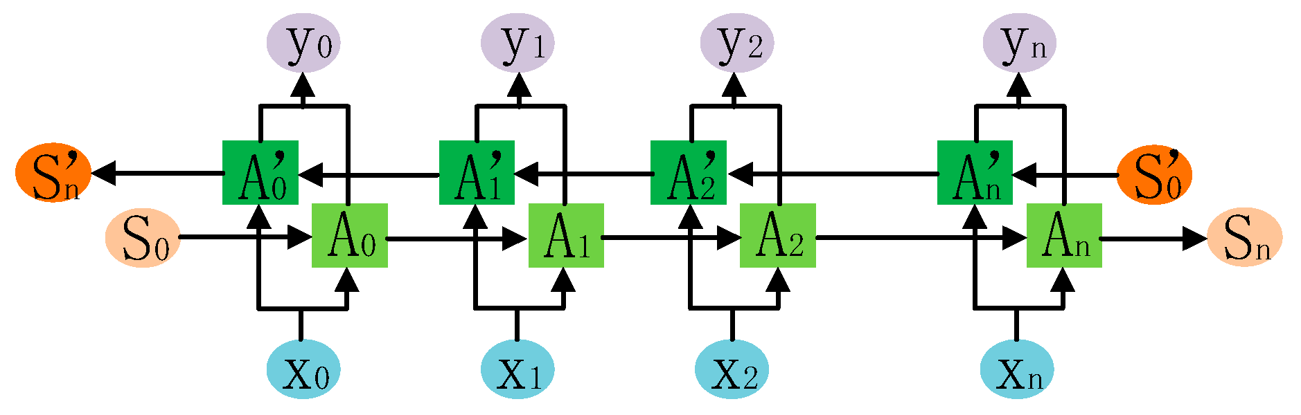
- (2)
- BLSTM
- (1)
- Training
- (2)
- Forecasting
3. Case Study
3.1. Results of Feature Selection
3.2. Comparison of the WPP Results Based on BPNN, LSTM, and BLSTM
4. Conclusions
- (1)
- Based on the data of the wind farm cluster and the 302,016 features in the paper, the feature selection and validation results show that the WPP errors of the wind farm cluster first drop sharply and then rise slowly with the increase in the number of features (Figure 8a). When the timescale of WPP is different, the number of optimal features and the optimal feature sets are different (Figure 10).
- (2)
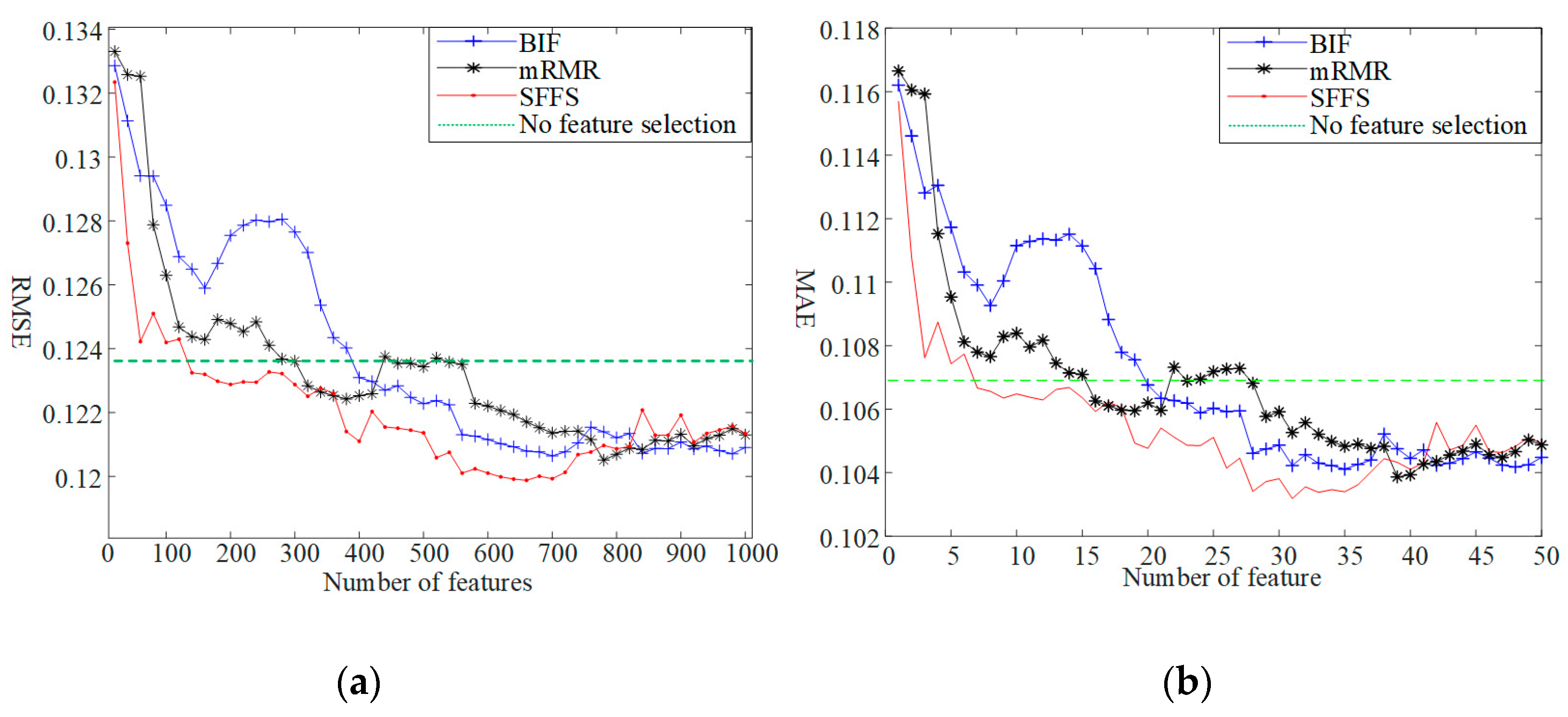
- The comparison of BIF-, mRMR-, and SFFS-based feature selection shows that the SFFS method selects more effective features than the other two methods.
- (3)
- When the number of the features selected by the SFFS method is about 130, the WPP accuracy is higher than that without feature construction and selection. When the number of selected features is about 660, the optimal accuracy is achieved, which is 0.37% lower than that without feature construction and selection (Figure 9). Compared with no feature construction and selection, after feature construction and selection, the errors of different prediction models have different degrees of decline (Figure 8, Figure 9 and Figure 10).
- (4)
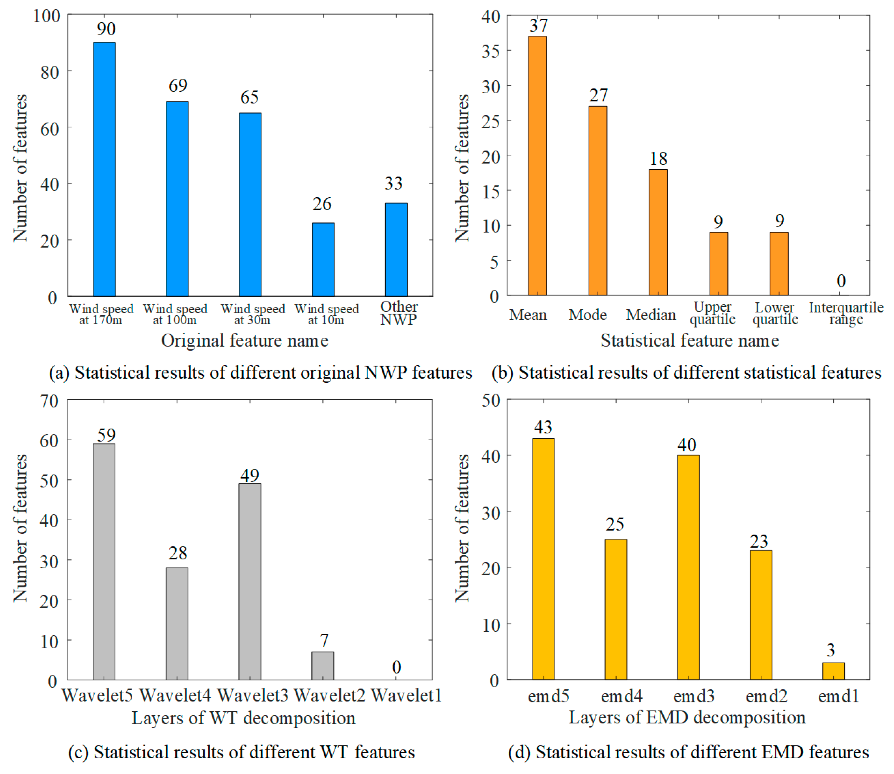
- The results of statistical analysis of the optimal feature set show that the following features are effective for the overall WPP modeling of wind farm clusters: wind speed of the height of the wind turbine hub, statistical features reflecting the overall situation of the wind farm cluster, low-frequency features in the frequency decomposition features, and so on (Figure 12).
- (5)
- Based on SFFS feature selection, a short-term WPP model for wind farm clusters based on BLSTM is presented in this paper. The case study demonstrates that BLSTM shows higher WPP accuracy than LSTM (Figure 13). Compared with LSTM, BLSTM can predict from both historical and future directions, which contributes to the outstanding performance of reducing the phase errors (Figure 14).
Author Contributions
Funding
Institutional Review Board Statement
Informed Consent Statement
Conflicts of Interest
References
- Wiser, R.; Bolinger, M. 2019 Wind Technologies Market Report; Lawrence Berkeley National Laboratory: Foshan, China, 2020.
- Cutler, N.J.; Outhred, H.R.; MacGill, I.F.; Kepert, J.D. Predicting and presenting plausible future scenarios of wind power production from numerical weather prediction systems: A qualitative ex ante evaluation for decision making. Wind Energy 2011, 15, 473–488. [Google Scholar] [CrossRef]
- Lobo, M.G.; Sanchez, I. Regional wind power forecasting based on smoothing techniques, with application to the Spanish peninsular system. IEEE Trans. Power Syst. 2012, 27, 1990–1997. [Google Scholar] [CrossRef]
- Zhang, Y.; Xu, Y.; Zhou, X.; Guo, H.; Zhang, X.; Chen, H. Compressed air energy storage system with variable configuration for accommodating large-amplitude wind power fluctuation. Appl. Energy 2019, 239, 957–968. [Google Scholar] [CrossRef]
- Burgas, L.; Colomer, J.; Melendez, J.; Gamero, F.I.; Herraiz, S. Integrated Unfold-PCA Monitoring Application for Smart Buildings: An AHU Application Example. Energies 2021, 14, 235. [Google Scholar] [CrossRef]
- Drew, R.; Cannon, J.; Barlow, F.; Coker, J.; Frame, H.A. The importance of forecasting regional wind power ramping: A case study for the UK. Renew. Energy 2017, 114, 1201–1208. [Google Scholar] [CrossRef]
- Li, Z.; Han, X.; Yang, M.; Ma, Y. Multi-stage power source and grid coordination planning method considering grid uniformity. Glob. Energy Interconnect. 2020, 3, 303–312. [Google Scholar] [CrossRef]
- Chen, N.; Wang, Q.; Yao, L.; Zhu, L.; Tang, Y.; Wu, F.; Chen, M.; Wang, N. Wind power forecasting error-based dispatch method for wind farm cluster. J. Mod. Power Syst. Clean Energy 2013, 1, 65–72. [Google Scholar] [CrossRef]
- Nedaei, M.; Assareh, E.; Walsh, P.R. A comprehensive evaluation of the wind resource characteristics to investigate the short term penetration of regional wind power based on different probability statistical methods. Renew. Energy 2018, 128, 362–374. [Google Scholar] [CrossRef]
- Hong, Y.-Y.; Rioflorido, C.L.P.P. A hybrid deep learning-based neural network for 24-h ahead wind power forecasting. Appl. Energy 2019, 250, 530–539. [Google Scholar] [CrossRef]
- Feng, C.; Cui, M.; Hodge, B.-M.; Zhang, J. A data-driven multi-model methodology with deep feature selection for short-term wind forecasting. Appl. Energy 2017, 190, 1245–1257. [Google Scholar] [CrossRef]
- Ekren, O.; Ekren, B.Y. Size optimization of a PV/wind hybrid energy conversion system with battery storage using simulated annealing. Appl. Energy 2010, 87, 592–598. [Google Scholar] [CrossRef]
- Lumbreras, S.; Ramos, A. Offshore wind farm electrical design: A review. Wind Energy 2012, 16, 459–473. [Google Scholar] [CrossRef]
- Şişbot, S.; Turgut, Ö.; Tunç, M.; Çamdalı, Ü. Optimal positioning of wind turbines on Gökçeada using multi-objective genetic algorithm. Wind Energy 2009, 13, 297–306. [Google Scholar] [CrossRef]
- Antal, E.; Tillé, Y. Simple random sampling with over-replacement. J. Stat. Plan. Inference 2011, 141, 597–601. [Google Scholar] [CrossRef]
- Bayat, A.; Bagheri, A. Optimal active and reactive power allocation in distribution networks using a novel heuristic approach. Appl. Energy 2019, 233–234, 71–85. [Google Scholar] [CrossRef]
- Zhang, C.; Zhou, J.; Li, C.; Fu, W.; Peng, T. A compound structure of ELM based on feature selection and parameter optimization using hybrid backtracking search algorithm for wind speed forecasting. Energy Convers. Manag. 2017, 143, 360–376. [Google Scholar] [CrossRef]
- Ma, Y.; Han, X.; Yang, M.; Lee, W. Multi-timescale robust dispatching for coordinated automatic generation control and energy storage. Glob. Energy Interconnect. 2020, 3, 355–364. [Google Scholar] [CrossRef]
- Aydemir, O.; Ergün, E. A robust and subject-specific sequential forward search method for effective channel selection in brain computer interfaces. J. Neurosci. Methods 2019, 313, 60–67. [Google Scholar] [CrossRef] [PubMed]
- Choi, K.-S.; Zeng, Y.; Qin, J. Using sequential floating forward selection algorithm to detect epileptic seizure in EEG signals. In Proceedings of the 2012 IEEE 11th International Conference on Signal Processing, Beijing, China, 21–25 October 2012; Volume 3, pp. 1637–1640. [Google Scholar]
- Ni, K.; Wang, J.; Tang, G.; Wei, D. Research and Application of a Novel Hybrid Model Based on a Deep Neural Network for Electricity Load Forecasting: A Case Study in Australia. Energies 2019, 12, 2467. [Google Scholar] [CrossRef]
- Li, D.; Mei, F.; Zhang, C.; Sha, H.; Zheng, J. Self-Supervised Voltage Sag Source Identification Method Based on CNN. Energies 2019, 12, 1059. [Google Scholar] [CrossRef]
- Li, C.; Ding, Z.; Yi, J.; Lv, Y.; Zhang, G. Deep Belief Network Based Hybrid Model for Building Energy Consumption Prediction. Energies 2018, 11, 242. [Google Scholar] [CrossRef]
- Delgado, I.; Fahim, M. Wind Turbine Data Analysis and LSTM-Based Prediction in SCADA System. Energies 2020, 14, 125. [Google Scholar] [CrossRef]
- Liu, P.; Zheng, P.; Chen, Z. Deep Learning with Stacked Denoising Auto-Encoder for Short-Term Electric Load Forecasting. Energies 2019, 12, 2445. [Google Scholar] [CrossRef]
- Zheng, H.; Yuan, J.; Chen, L. Short-Term Load Forecasting Using EMD-LSTM Neural Networks with a Xgboost Algorithm for Feature Importance Evaluation. Energies 2017, 10, 1168. [Google Scholar] [CrossRef]
- He, F.; Zhou, J.; Feng, Z.-K.; Liu, G.; Yang, Y. A hybrid short-term load forecasting model based on variational mode decomposition and long short-term memory networks considering relevant factors with Bayesian optimization algorithm. Appl. Energy 2019, 237, 103–116. [Google Scholar] [CrossRef]
- Huang, C.; Huang, H.; Li, Y. A Bi-Directional LSTM prognostics method under multiple operational conditions. IEEE Trans. Ind. Electron. 2019, 66, 8792–8802. [Google Scholar] [CrossRef]
- Graves, A.; Fernández, S.; Schmidhuber, J. Bidirectional LSTM Networks for Improved Phoneme Classification and Recognition; Springer Science and Business Media LLC: Berlin/Heidelberg, Germany, 2005; pp. 799–804. [Google Scholar]
- Graves, A.; Jaitly, N.; Mohamed, A.-R. Hybrid speech recognition with Deep Bidirectional LSTM. In Proceedings of the 2013 IEEE Workshop on Automatic Speech Recognition and Understanding, Olomouc, Czech Republic, 8–12 December 2013; pp. 273–278. [Google Scholar]
- Frinken, V.; Fischer, A.; Baumgartner, M.; Bunke, H. Keyword spotting for self-training of BLSTM NN based handwriting recognition systems. Pattern Recognit. 2014, 47, 1073–1082. [Google Scholar] [CrossRef]
- Baldi, P.; Brunak, S.; Frasconi, P.; Soda, G.; Pollastri, G. Exploiting the past and the future in protein secondary structure prediction. Bioinformatics 1999, 15, 937–946. [Google Scholar] [CrossRef]
- Liu, S.; Shi, R.; Huang, Y.; Li, X.; Li, Z.; Wang, L.; Mao, D.; Liu, L.; Liao, S.; Zhang, M.; et al. A Data-Driven and Data-Based Framework for Online Voltage Stability Assessment Using Partial Mutual Information and Iterated Random Forest. Energies 2021, 14, 715. [Google Scholar] [CrossRef]
- Xu, Q.; He, D.; Zhang, N.; Kang, C.; Xia, Q.; Bai, J.; Huang, J. A Short-Term Wind Power Forecasting Approach with Adjustment of Numerical Weather Prediction Input by Data Mining. IEEE Trans. Sustain. Energy 2015, 6, 1283–1291. [Google Scholar] [CrossRef]
- Gacav, C.; Benligiray, B.; Topal, C. Sequential forward feature selection for facial expression recognition. In Proceedings of the 2016 24th Signal Processing and Communication Application Conference (SIU), Zonguldak, Turkey, 16–19 May 2016; pp. 1481–1484. [Google Scholar]
- Setiawan, D.; Kusuma, W.A.; Wigena, A.H. Sequential forward floating selection with two selection criteria. In Proceedings of the 2017 International Conference on Advanced Computer Science and Information Systems (ICACSIS), Bali, Indonesia, 28–29 October 2017; pp. 395–400. [Google Scholar]
- Gan, J.Q.; Hasan, B.A.S.; Tsui, C.S.L. A filter-dominating hybrid sequential forward floating search method for feature subset selection in high-dimensional space. Int. J. Mach. Learn. Cybern. 2012, 5, 413–423. [Google Scholar] [CrossRef]
- Wu, Z.; Du, X.; Gu, W.; Ling, P.; Liu, J.; Fang, C. Optimal Micro-PMU Placement Using Mutual Information Theory in Distribution Networks. Energies 2018, 11, 1917. [Google Scholar] [CrossRef]
- Iranmanesh, H.; Abdollahzade, M.; Miranian, A. Mid-Term Energy Demand Forecasting by Hybrid Neuro-Fuzzy Models. Energies 2011, 5, 1–21. [Google Scholar] [CrossRef]
- Ning, Y.; Wu, Z.; Li, R.; Jia, J.; Xu, M.; Meng, H.; Cai, L. Learning cross-lingual knowledge with multilingual BLSTM for emphasis detection with limited training data. In Proceedings of the 2017 IEEE International Conference on Acoustics, Speech and Signal Processing (ICASSP), New Orleans, LA, USA, 5–9 March 2017; pp. 5615–5619. [Google Scholar]


| Feature Types | Quantity | Description |
|---|---|---|
| Wind speed | 4 | Wind speed at 170 m, 100 m, 30 m, 10 m |
| Wind direction | 4 | Wind direction at 170 m, 100 m, 30 m, 10 m |
| Temperature | 1 | Atmospheric temperature |
| Humidity | 1 | Atmospheric humidity |
| Pressure | 1 | Sea-level pressure |
| Feature Types | Quantity | Description |
|---|---|---|
| Mean | 11 | Mean of 11 original features for 20 wind farms |
| Mode | 11 | Mode of 11 original features for 20 wind farms |
| Upper quartile | 11 | Upper quartile of 11 original features for 20 wind farms |
| Median | 11 | Median of 11 original features for 20 wind farms |
| Lower quartile | 11 | Lower quartile of 11 original features for 20 wind farms |
| Interquartile range | 11 | Interquartile range of 11 original features for 20 wind farms |
| Feature Type | Quantity | Main Frequency Components |
|---|---|---|
| wavelet1 | 27,456 | >4.55 × 10⁻⁵ Hz |
| wavelet2 | 27,456 | 3.35~4.55 × 10⁻⁵ Hz |
| wavelet3 | 27,456 | 2.25~3.35 × 10⁻⁵ Hz |
| wavelet4 | 27,456 | 1.15~2.25 × 10⁻⁵ Hz |
| wavelet5 | 27,456 | <1.15 × 10⁻⁵ Hz |
| Emd1 | 27,456 | >1.5 × 10⁻⁵ Hz |
| Emd2 | 27,456 | 1.5~1.27 × 10⁻⁵ Hz |
| Emd3 | 27,456 | 1.27~0.7 × 10⁻⁵ Hz |
| Emd4 | 27,456 | 0.7~0.2 × 10⁻⁵ Hz |
| Emd5 | 27,456 | <0.2 × 10⁻⁵ Hz |
| NWP_NUM | CAP(MW) | NWP_NUM | CAP(MW) |
|---|---|---|---|
| CN0014 | 49.5 | CN0263 | 99.0 |
| CN0016 | 99.0 | CN0286 | 99.0 |
| CN0018 | 94.5 | CN0029 | 48.0 |
| CN0017 | 102.0 | CN0351 | 172.5 |
| CN0015 | 90.0 | CN0437 | 99.0 |
| CN0029 | 79.5 | CN0505 | 198.18 |
| CN0136 | 99.0 | CN0351 | 150.0 |
| CN0136 | 69.5 | CN0287 | 100.0 |
| CN0287 | 148.5 | CN0449 | 96.0 |
| CN0199 | 297.0 | CN0449 | 97.5 |
| NUM | NAME | FREQ | WIND FARM |
|---|---|---|---|
| 1 | 170 m wind speed | wavelet1 | Wind farm 10 |
| 2 | 30 m wind speed | emd4 | Wind farm 11 |
| 3 | 10 m wind speed | emd2 | Wind farm 7 |
| 4 | 170 m wind speed | emd3 | Wind farm 19 |
| … | … | … | … |
| 660 | 10 m wind speed | emd2 | Wind farm 18 |
Publisher’s Note: MDPI stays neutral with regard to jurisdictional claims in published maps and institutional affiliations. |
© 2021 by the authors. Licensee MDPI, Basel, Switzerland. This article is an open access article distributed under the terms and conditions of the Creative Commons Attribution (CC BY) license (https://creativecommons.org/licenses/by/4.0/).
Share and Cite
Peng, X.; Cheng, K.; Lang, J.; Zhang, Z.; Cai, T.; Duan, S. Short-Term Wind Power Prediction for Wind Farm Clusters Based on SFFS Feature Selection and BLSTM Deep Learning. Energies 2021, 14, 1894. https://doi.org/10.3390/en14071894
Peng X, Cheng K, Lang J, Zhang Z, Cai T, Duan S. Short-Term Wind Power Prediction for Wind Farm Clusters Based on SFFS Feature Selection and BLSTM Deep Learning. Energies. 2021; 14(7):1894. https://doi.org/10.3390/en14071894
Chicago/Turabian StylePeng, Xiaosheng, Kai Cheng, Jianxun Lang, Zuowei Zhang, Tao Cai, and Shanxu Duan. 2021. "Short-Term Wind Power Prediction for Wind Farm Clusters Based on SFFS Feature Selection and BLSTM Deep Learning" Energies 14, no. 7: 1894. https://doi.org/10.3390/en14071894
APA StylePeng, X., Cheng, K., Lang, J., Zhang, Z., Cai, T., & Duan, S. (2021). Short-Term Wind Power Prediction for Wind Farm Clusters Based on SFFS Feature Selection and BLSTM Deep Learning. Energies, 14(7), 1894. https://doi.org/10.3390/en14071894