Article

Application of a New Dispatch Methodology to Identify the Influence of Inertia Supplying Wind Turbines on Day-Ahead Market Sales Volumes

Wind Energy Technology Institute (WETI), Flensburg University of Applied Sciences, 24943 Flensburg, Germany
*
Author to whom correspondence should be addressed.
Energies 2021, 14(5), 1255; https://doi.org/10.3390/en14051255
Submission received: 19 January 2021 / Revised: 15 February 2021 / Accepted: 18 February 2021 / Published: 25 February 2021
(This article belongs to the Special Issue Grid Services with Wind Turbines and the Resulting Mechanical Loads)

Abstract

:
Power system inertia is an essential part of grid frequency control. The number of synchronously connected machines, which inherently provide inertia, is decreasing due to the transition to renewable energies. Conventional generation units are being replaced by renewable generation units which are connected to the grid via frequency converters. Some power systems already suffer from too little power system inertia. Hence, inertia is a valuable yet non-traded commodity. A day-ahead dispatch methodology to secure power system inertia was developed and is applied and assessed in this work. Day-ahead market data of the combined market of the Republic of Ireland and Northern Ireland is used. If the superimposition of sell and buy bids results in insufficient inertia, the dispatch algorithm is applied. In decreasing price order, non-inertia-providing sell bids get replaced by the following sell bids in the merit order. The iterative process is repeated until sufficient inertia is in the system. The provision of synthetic inertia by wind turbines is considered in the process. The costs for additional stored kinetic energy for the assessed time periods and scenarios result in costs ranging from 1.02 to 4.49 EUR/kgm2.

1. Introduction

The absolute need to decarbonise energy systems is indisputable. In order to achieve greenhouse gas emission targets, the power system generation mix shifts from a generation mix based on fossil fuel driven generation sources to a mix based on renewable generation sources [1]. The increasing share of renewable energy sources challenges power system operators and authorities [1], and power markets [2]. An important challenge is the maintenance of grid frequency controllability due to decreasing power system inertia [1].
Power system inertia is an essential, yet passive part of grid frequency control [1]. The grid frequency itself is the indicator for power balance in AC power systems [3]. If power supply and power demand, including grid losses, are balanced, the grid frequency is constant [3]. In case power supply surpasses power demand, the grid frequency increases and vice versa [3]. The grid frequency is a representation of the rotational speed of all synchronously connected rotating masses in power systems [3]. The speed with which the grid frequency changes in the event of a power imbalance, commonly known as the rate of change of frequency (ROCOF), is determined by the synchronously connected machines with their rotating masses, i.e., their moments of inertia [3]. Higher power system inertia decreases the rate with which the grid frequency changes [1]. If the grid frequency increases, the rotational speed of the synchronously connected machines increases and kinetic energy is stored in the rotational motion [1]. If the grid frequency decreases, the rotational speed decreases and kinetic energy is released into the grid [1]. Thereby, the speed with which the grid frequency changes is reduced and units providing grid frequency stability services, like frequency containment reserves, are supplied with sufficient time to adapt their power generation output [1].
Most synchronously connected machines are synchronous generators of conventional power plants [1]. Power system inertia is supplied by synchronously connected units of power consumers too [4]. Due to the replacement of fossil fuel power plants, the number of synchronous generators and thereby the amount of inertia in power systems is decreasing. State of the art wind turbines (WT) and photovoltaic systems are connected to the grid via frequency converters [1]. Hence, they do not provide an inertia contribution in the event of a power imbalance [
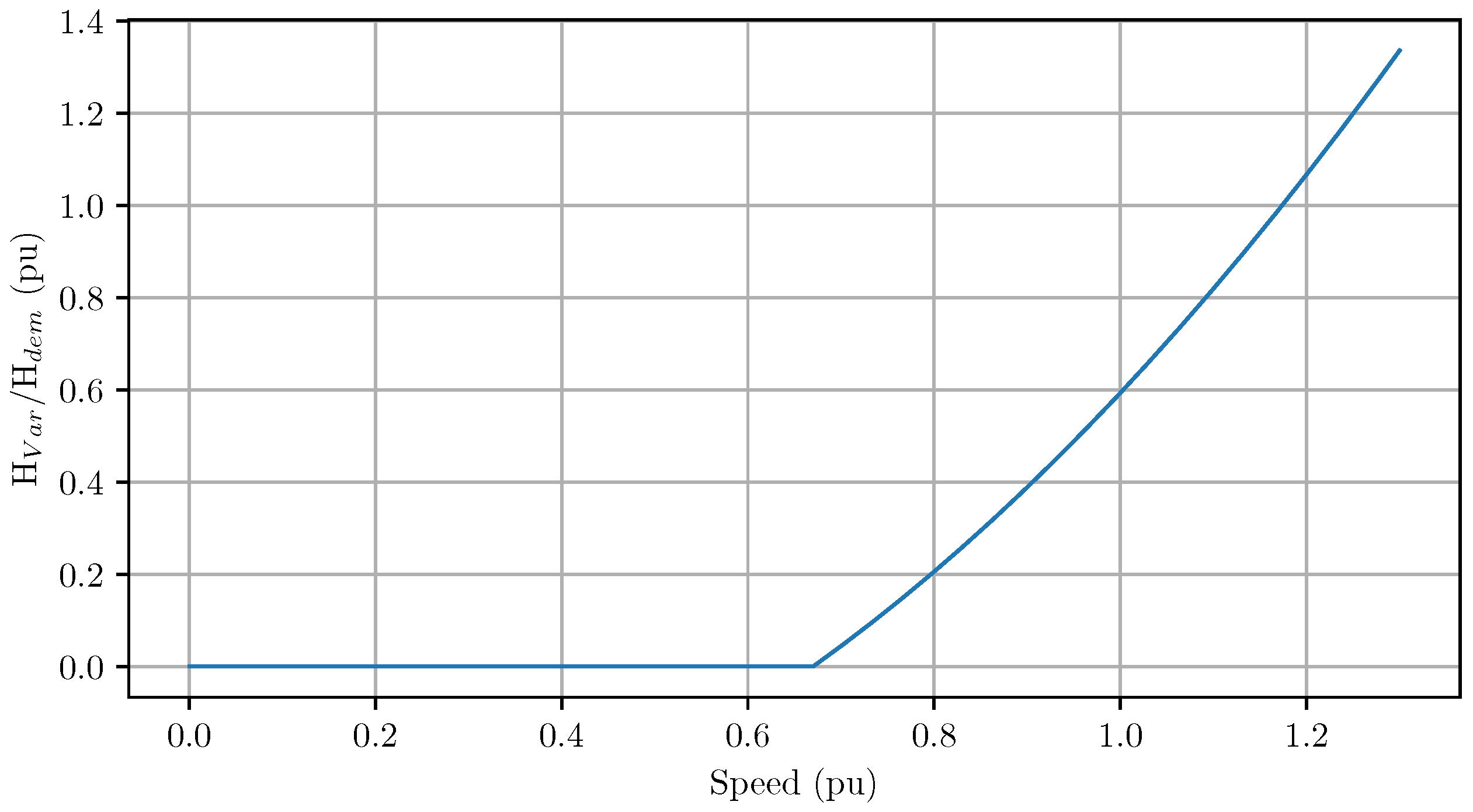
1]. However, WT are able to mimic the behaviour of a synchronous machine in the event of a power imbalance by applying additional control strategies and changing the rotational speed of the WT rotor [5]. This is commonly known as synthetic inertia (SI) [1]. A novel approach to provide SI continuously with WT [6], will be applied in this work.
Some transmission system operator (TSO) already demand generation sources like WT to provide an inertia contribution, e.g., in the event of an under frequency situation [7]. The Irish power system, meaning the interconnected systems of the Republic of Ireland and Northern Ireland, is characterised by a high share of non-synchronous generation sources, mostly WT [8]. During certain hours, power generation from renewable sources has to be turned-off or dispatched down for power system security reasons [8]. Statistics regarding dispatched down generation WT energy is published frequently by the TSO [9]. Reasons for such measures are localised network reasons (constraints) or system-wide reasons (curtailment), such as high non-synchronous penetration or low power system inertia [8]. Hence, as the share of renewable generation sources emerges in power systems all around the world, the present all-island Irish power system represents a future state of other systems. As the Republic of Ireland and Northern Ireland are both industrialised countries, research findings can be transferred and applied on larger power systems. Still, the sizes and number of units of the system are perfectly manageable for research purposes.
Inertia is not yet a tradeable commodity nor is it economically researched in detail [
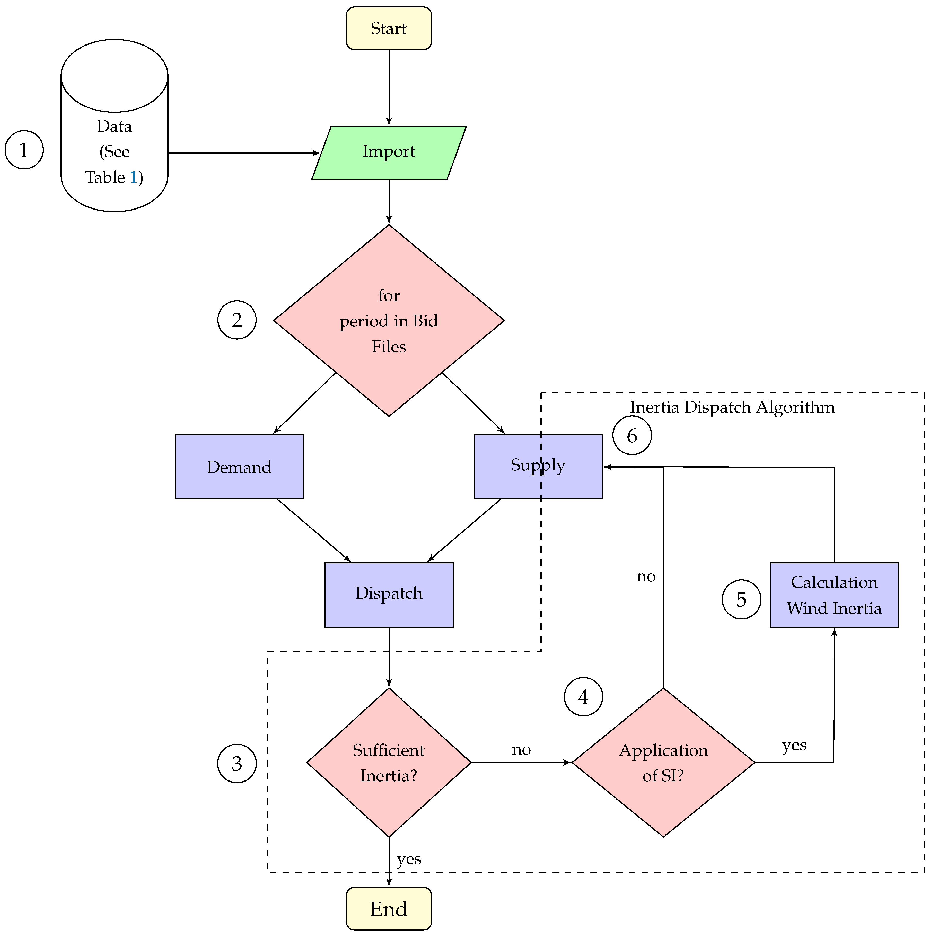
2]. A novel dispatch methodology to secure grid frequency controllability by sufficient power system inertia is introduced in [10]. This dispatch methodology calculates the amount of inertia based on trading results of the day-ahead spot market [10]. In the event of insufficient inertia, the most expensive non-inertia supplying unit is replaced by the following unit in the merit order whose bid was previously outside the market balance [10]. This process is repeated until the necessary quantity of inertia is achieved [10].
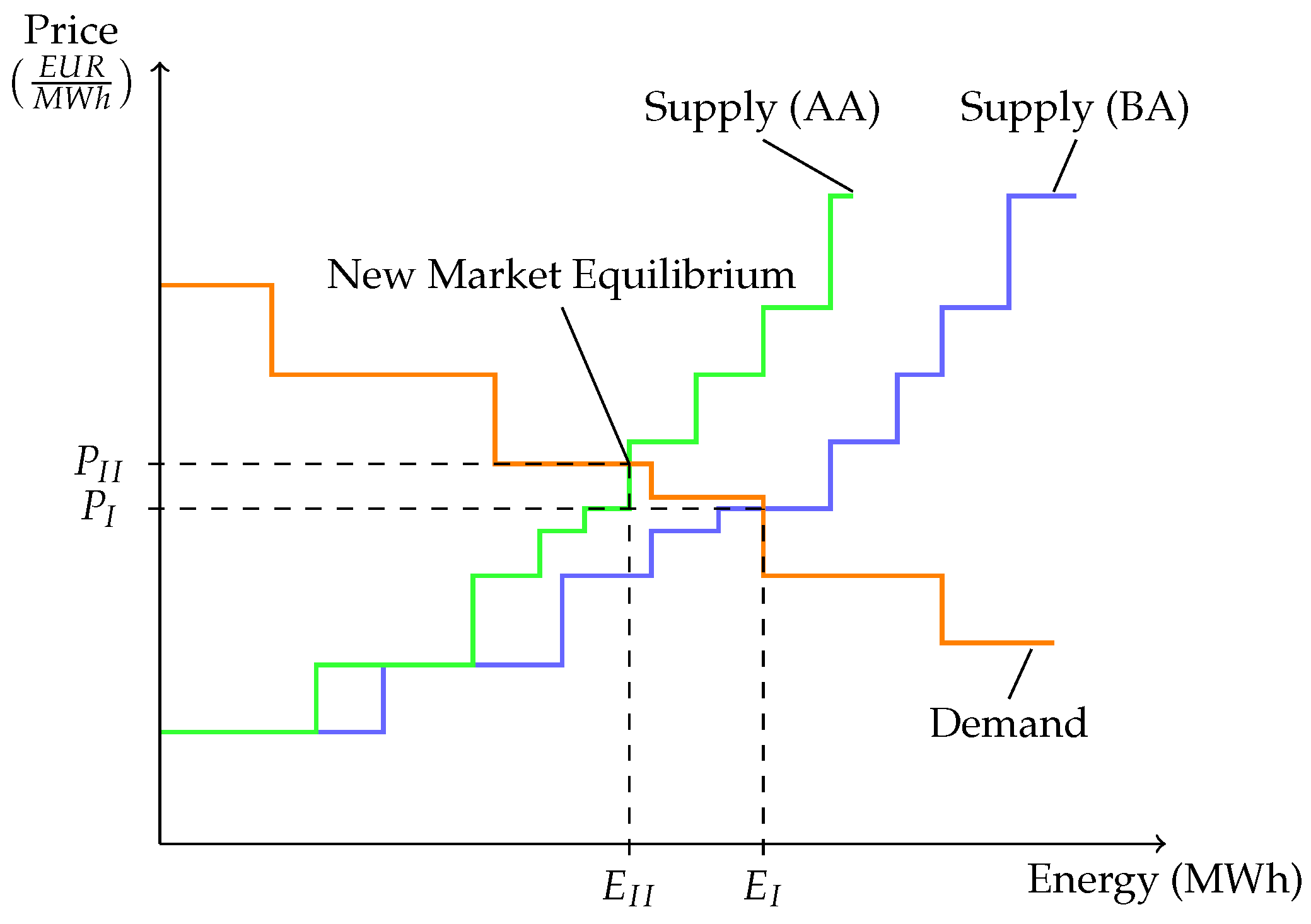
The purpose of the work at hand was to apply a novel inertia dispatch methodology. The methodology determines the lowest day-ahead market dispatch cost solution whilst ensuring a sufficient amount of inertia. Additional inertia due to the application of the methodology can be economically quantified. A further research contribution is the introduction and assessment of SI provided by WT as part of the dispatch solution. Therefore, available day-ahead market data of the single electricity market of the Republic of Ireland and Northern Ireland are used. A period of six months is analysed. The applied methodology results, if necessary due to low power system inertia, in a new market equilibrium. Therefore, the upcoming Section 2 first reviews system inertia in dispatch modeling publications followed by an introduction to SI provision from WT. Section 3 describes the researched dispatch methodology functionality and applied data. Results are presented in Section 4 and discussed in Section 5. Section 6 concludes the findings.

2. Literature Review

In the following, research regarding power system inertia as part of dispatch modeling is introduced. Afterwards, the methodology for continuous provision of emulated inertia by WT is explained.

2.1. Inertia in Power System Dispatch Modeling

Various publication attempt to incorporate frequency response as a system security constraint into dispatch problems. Power system inertia, being the passive part of power frequency response services, is a variable co-optimised by the dispatch model.
One of the first works considering costs for power system security is outlined by O’Sullivan and O’Mally [11]. They propose a new economic dispatch methodology for a small isolated power system. Costs for the provision of sufficient reserve to prevent load shedding is assessed with costs associated with load shedding, thus dispatch costs against costs for load shedding. The cases researched consider the loss of the three largest units in the system. However, the work does not consider whether sufficient power system inertia is available for power frequency control. Additionally, the proposed methodology is not compatible with modern market dispatch algorithms as stated in [12]. Therefore, Doherty et al. propose a novel approach to ensure frequency control which is compatible with modern market clearing engines [12]. A ROCOF and a lower bound power frequency constraint is proposed, being co-optimised in a linear programming market-clearing algorithm. The system assessed, is the all island system of the Republic of Ireland and Northern Ireland. It is concluded that the frequency-based security constraints is successfully included into the proposed linear programming dispatch algorithm. However, it can not be applied in large and small power systems equally. Whilst considering stored kinetic energy for power frequency control, only synchronous inertia is considered. A novel stochastic economic dispatch model to optimally schedule energy and reserve is introduced by Lee et al. [13]. Reserves are geographically co-optimised and capacity left for power increase and ramp rates on system frequency. Using generic cost data, the model outcome is assessed against ERCOT network and load data from summer 2011. A shortfall in synchronous inertia within the unit commitment and economic dispatch model PLEXOS for Ireland and Northern Ireland is analysed by Daly et al. [14]. Therefore, a static and a dynamic inertia constrained based on the largest in- or outfeed is formulated to limit the ROCOF. Whilst optimising for system costs, additionally, wind curtailment is minimised. It is concluded that there is the need to formulate specific inertial policy. Although, the work assesses wind curtailment reduction, SI is not considered for power frequency stability. Teng et al. formulated a simplified dynamic frequency model to formulate constraints incorporated in a stochastic unit commitment model [15]. The uncertainty due to wind feed-in on power system inertia is quantified and taken into account in the constraint formulation. Scheduling energy production, standing/spinning reserve and inertia dependent fast frequency response are cost-optimised on the power system of Great Britain for the year 2030. An important conclusion is that “synthetic inertia from wind turbines is believed to play an important role in supporting the frequency performance in the future low carbon power system” [15]. On a higher spatial level, namely, the 28 member states of the EU as in 2017, Collins et al. assessed the robustness of the power sector based on the PRIMES-REF scenario of the year 2040 applying higher technical and temporal resolution [16]. The unit commitment and economic dispatch tool PLEXOS is used to quantify variable renewable electricity curtailment, levels of interconnector congestion and wholesale electricity prices [16]. Considered as well is the maintenance of sufficient levels of power system inertia for frequency control. However, SI from WT is not considered to contribute to frequency control. Analysing the ERCOT power system, a mixed-integer linear program was formulated using PLEXOS by Johnson et al. resulting in unit commitment and dispatch model to quantify system inertia [17]. A system inertia constraint was added to the unit commitment and dispatch model. The results show that “models without a system inertia constraint are not fully capturing the impact of variable renewable energy on the generation mix” [17]. More importantly: “As grids integrate more renewable energy, relying on the current method of delivering inertia will see escalating costs, which demonstrates the value of integrating new sources of inertia, like synthetic inertia from wind turbines” [17].
As indicated by the literature review, there is a growing interest in modeling system inertia in power systems, and including inertia deployment as part of the dispatch problem. A valuable research contribution of the work at hand is the integration of SI providing WT into the modeling process and assessing its influence on power prices. Further, the presented inertia dispatch methodology allows for a cost assessment of the additionally supplied inertia. Instead of using generic cost data as in previous research, this work applies actual bidding data from the Irish power market.

2.2. Synthetic Inertia by Wind Turbines

Some power systems with a high level of frequency converter based generation already experience times with low power system inertia [1]. TSO reacted to this development and require WT to provide services like fast frequency response or SI; one of the first beeing Hydro Québec TransÉnergie [7]. The definition of SI under TSO is not consistent [6]. Basically, three different methods are used: first, the additional power output of the WT when the power frequency exceeds a defined ROCOF threshold; second, power increase is activated when a grid frequency threshold is exceeded and third, the emulation of the behavior of a synchronous generator independently from ROCOF or grid frequency thresholds [6].
Emulation of the behaviour of a synchronous generator using WT applying different control strategies has been presented and discussed in literature for many year [18]. A novel, more system relevant expedient control strategy to provide SI continuously is presented by Gloe et al. [6], which will be used in this work, and is therefore briefly introduced in the following: A general approach to provide SI with WT is to adapt the electric power output based on the ROCOF. This deviation of the electric power from the wind power causes the WT rotor to release or store kinetic energy, and hence change the rotational speed of the rotor. As a result, the WT might run at a non-optimal rotational speed, which in the worst case, leads to the disconnection of the WT from the power system. Hence, the inertia support of the WT and the non-inertia related power feed-in is lost. Thus, the grid situation from the TSO’s point of view changes for the worse. WT operators and TSO have different interests when it comes to the provision of SI. WT operators want to maximize the turbines energy yield, whilst grid operators require a reliable provision of SI. To unite both interests, the variable inertia ( H v a r ) controller was developed by Gloe et al. [6]. The authors propose to scale the inertia constant to be emulated ( H d e m ) with the operating point of the WT, considering the cut-in speed of the WT. The inertia constant is a measure for the units inertia, indicating the theoretical time a synchronous generator is able to provide its nominal power only by the generators stored kinetic energy [1]. H d e m is defined by the TSO based on the power system requirements. H v a r / H d e m is thus calculated as follows:
H v a r H d e m = 0.5 · J W T · ( ω a c t u a l , W T 2 ω c u t i n , W T 2 ) 0.5 · J W T · ( ω r a t e d , W T 2 ω c u t i n , W T 2 )
Figure 1 visualizes the relation of the variable inertia constant, H v a r , with respect to the demanded inertia constant, H d e m and the operating range of the WT. By design of the variable H controller, the TSO is ensured to be provided with sufficient SI. At the same time, the TSO has not to fear the loss of WT power feed-in due to the rotor speed dropping below ω c u t i n , W T whilst providing SI. On the other side, the impact on the energy yield for the WT operator is reduced to a minimum. Hence, the control strategy of Gloe et al. compensates for the possible disconnection of WT due to too low rotor speed which previous research did not account for.

3. Data and Methods

In the upcoming subsections the methodology of the applied inertia dispatch algorithm is presented and how SI is modeled and incorporated. Assumptions regarding the applied data are presented and the developed scenarios and data itself.

3.1. Inertia Dispatch Methodology

The basic functionality of the inertia dispatch methodology is introduced and discussed in detail in a paper published in 2018 [10]. The following subsection summarises the essence of the inertia dispatch methodology, its functionality and presenting how it is applied in this work. It is illustrated in Figure 2.
The process is started by importing all data (see step 1 in Figure 2) as listed in Table 1 and further detailed in Section 3.3. Thereafter, for every trading period of all imported bid files (see step 2 in Figure 2) all buy bids for electrical energy for a given trading period are arranged increasingly by the price (see blue graph in Figure 3). Sell bids are arranged decreasingly (see orange graph in Figure 3). The intersection of the demand and supply curves result in the market equilibrium. The market equilibrium indicates the market price ( P I ) and the amount of traded energy ( E I ). Once the market equilibrium is achieved, the potential stored kinetic energy of the bidding unit is calculated. For each bidding unit in the Irish power market, the rated power is known (see list of registered units in Table 1) [19]. The inertia constant for the respective unit is derived from literature (see Table 2). The product of the inertia constant and the rated power results in the stored kinetic energy. The algorithm checks, whether sufficient inertia is provided by the dispatched power generation units (see step 3 in Figure 2). In case, the calculated stored kinetic energy is below a minimum requirement defined by the TSO, the inertia dispatch methodology is applied. Otherwise, the market equilibrium for the following trading period is generated.
In case the inertia calculation (step 3 in Figure 2) results in an insufficient amount of power system inertia as it is predefined by the TSO, the inertia dispatch methodology is applied. At first, it is checked whether SI by WT is considered (step 3 in Figure 2) in the researched scenario. If SI by WT is not considered, step 5 (calculation of wind inertia) is skipped. Otherwise, SI by WT is calculated as explained in detail in Section 3.2. This distinction is important, as it is the purpose of the work at hand to assess the influence of SI from WT on power prices. Hence, in the base scenarios step 5 is skipped and to analyse the influence of SI step 5 is executed.
With or without applying SI calculation (step 5 in Figure 2), the supply bid curve is restructured (see step 6 in Figure 2) as explained in the following. In the first step, the most expensive, non-inertia-providing generation unit with a price equal to or below the market equilibrium price is removed from the merit order. Next, in order to supply the energy demand, the following generation unit in the merit order is selected and a new market equilibrium is achieved. Thereby, the adapted supply curve is shifted to the left. The market price is then equal to or higher compared to the previous market price. Afterwards, the amount of inertia is calculated again, which is equal to or higher compared to the previous one. If the newly calculated amount of inertia is still insufficient, i.e., below the defined value of the TSO, the whole process is executed and iterated until sufficient inertia is achieved (see the green graph in Figure 4). Hence, a new market equilibrium (see P I I and E I I in Figure 4). By this process, the grid is provided with sufficient amount of inertia to ensure controllability of the grid frequency.
Even though the methodology of models reviewed in Section 2 is published, the used tools and most of the model itself remains a “black box”. There are many reasons to fully publish models and underlying code and simplify accessibility by using free software and tools [30]. Therefore, following the open science approach, the logic inertia dispatch methodology is translated into Python code. The methodology has previously not been used in any modeling environment. The files containing the full model are available on GitHub and published under the GNU General Public License v3.0 [31].

3.2. Modeling Synthetic Inertia for the Inertia Dispatch Methodology

The introduced inertia dispatch methodology did not include SI in the first place [10]. Nevertheless, it can easily be integrated. The inertia dispatch methodology only distinguishes whether a unit is providing inertia or not. Whether inertia is provided in the form of synchronous inertia from a synchronous generator or in the form of emulated inertia, i.e., SI, by a WT is of no matter. Therefore and for the purpose of the work at hand, the potential available SI from WT is calculated and integrated into the inertia dispatch methodology. Section 2.2 briefly introduces the continuous variable H controller which is used to calculate the potential available kinetic energy from WT in the power system of Ireland. Figure 5 illustrates the methodology to calculate the potential available inertia of the WT as part of the inertia dispatch methodology as a whole depicted in Figure 2. Table 1 summarises the applied data.
Each bid of the merit order for the respective trading period, is checked to be a wind generation source given by information of the list of registered units (see step 1 in Figure 5). Afterwards, in step 2, information about the location of the wind source is gathered [20]. Having the location of the WT, wind data from the nearest wind measurement source (see Table 1-Wind measurement data and step 3 in Figure 5) is used to determine the power of the WT (see step 4 in Figure 5) [21]. Therefore, the power curve in per unit as depicted in Figure 6 from the NREL 5 MW WT is applied [22]. The normalized power is then used to determine the respective normalized rotational speed (see step 5 in Figure 5 and Figure 7). In the following step 6, the inertia constant is determined by using the normalized rotational speed vs. H v a r / H d e m characteristic (see Figure 1). The potential stored kinetic energy by the WT can finally be calculated by multiplying H v a r and the installed WT capacity. This process is executed for each wind unit bidding at the power market in the respective trading period.

3.3. Power Market Data and Scenarios

The intention of the work at hand is, to asses and apply the inertia dispatch methodology. Therefore, data provided by the power market operator of the combined market of the Republic of Ireland and Northern Ireland is used. The all-island power system of the Republic of Ireland and Northern Ireland was chosen to be researched, as it already today is characterised by little sources of synchronous inertia and, at the same time, having a high share of wind generation units installed. Additionally, it is a power system with a manageable number of generation units for research purposes and only being connected via HVDC transmission lines with other synchronous areas. The time period researched starts on 2020-03-06 and ends on 2020-09-21. It is assumed that a six month period covers most situations a power system experiences. Meaning, seasonal, weekly, daily patterns of power demand and wind speed and singularities like public holidays. Therefore, the researched time period is representative. Data provided by the market operator and from the ENTSO-E is incorporated without adjustments. A set of data of all registered units from April 2020 provides basic information like registered capacities and fuel types of the market participants [19]. Bid data containing sell and buy offers of all participants with quantity and price combinations are provided by the market operator [23]. Bids are offered in either Euro or in Pound Sterling [24]. The necessary exchange rate to convert currencies is provided in the market result data sets [23]. Data provided by the ENTSO-E is used to account for the inertia from generation units not traded on the day-ahead market [25]. Table 1 summarises the applied data.
Information about the moment of inertia of each generation unit is available neither through the power market operator nor through the TSO. Hence, inertia data per fuel type is derived from literature [27,28,29]. Table 2 provides an overview about the upper ( H h i g h ) and lower bound ( H l o w ) of the applicable range of inertia constants. Table 2 reveals that for some fuel types, a wide range of inertia constants is available. Without deeper insight into technical specifications of each generation unit, a precise allocation of the inertia constant is not possible. Hence, for the purpose of this work, two assumptions regarding the inertia constant per unit is made. The first assumption uses the lower bound values of Table 2 ( H l o w ). The second assumption uses the upper bound values ( H h i g h ). If only one value, i.e., not a range, is provided in Table 2, this value is applied in both cases.
The TSO of the Republic of Ireland and Northern Ireland indicates an operation limit of inertia in terms of kinetic energy ( E k i n , d e m ) [26]. At least 23,000 MWs have to be present in the whole system at any time [26]. The stored kinetic energy ( E k i n , i ) per synchronous unit can be calculated by multiplying the inertia constant of a generator ( H i ) with its rated apparent power ( S i ) [1]. The system-wide stored kinetic energy is calculated by summing up the individual kinetic energies of all synchronous generators.
It is not stated by the TSO whether inertia provided by power loads is taken into account. However, literature shows that about 20% of the average system inertia is supplied by power consumers [4,32]. To take this fact into account, two assumptions for the required inertia, in this case the required stored kinetic energy, are made. The first assumption is a required operation limit of kinetic energy of 23,000 MWs and the second assumption is an operation limit of kinetic energy of 18,400 MWs. The latter number takes a 20% inertia provision by power consumers into account.
Based on the assumptions made for the inertia constant per fuel type and for the required operation limit of kinetic energy, four scenarios sets are assessed as described in the following:
  • A combination of a high required operation limit of kinetic energy (23,000 MWs) and high inertia constants ( H h i g h ) per fuel type;
  • A combination of a high required operation limit of kinetic energy (23,000 MWs) and low inertia constants ( H l o w ) per fuel type;
  • A combination of a low required operation limit of kinetic energy (18,400 MWs) and high inertia constants ( H h i g h ) per fuel type;
  • A combination of a low required operation limit of kinetic energy (18,400 MWs) and low inertia constants ( H l o w ) per fuel type.
Each scenario set is then further divided into one scenario which does not contain SI from WT and one scenario which includes SI from WT. Hence, in total eight scenario are defined.

4. Results

In total, 4799 trading periods of the Irish day-ahead power market were researched by applying the inertia dispatch methodology. The analysis started on 2020-03-06 and ended on 2020-09-21. Table 3 sums up the overall results of the dispatch methodology application. Based on the combination of demanded kinetic energy by the TSO and whether inertia contribution from power consumers is applied ( E k i n , d e m = 23,000 MWs or E k i n , d e m = 18,400 MWs), the assumptions of the inertia constant per generator type ( H l o w or H h i g h ) and whether SI contribution is considered or not (SI or non-SI), the number of times where market balance results in insufficient kinetic energy varies significantly (see column Times of methodology application of Table 3). The outcome was 133 times up to 4683 times of insufficient inertia. Obviously, a combination of a lower demand for stored kinetic energy ( E k i n , d e m = 18,400 MWs), a higher assumed generator inertia constant ( H h i g h ) and the application of SI by WT results in significantly fewer times of insufficient power system inertia compared to less beneficial system conditions. For the combination of E k i n , d e m = 23,000 MWs, H l o w and no SI contribution by WT, 4683 out of 4799 times the market dispatch results in insufficient stored kinetic energy.
A similar pattern can be observed when considering the number of times the inertia dispatch algorithm is not able to meet the condition of sufficient system kinetic energy. The number of times no solution could be found ranged from 0 for two combinations ( E k i n , d e m = 18,400 MWs, H h i g h , non-SI and E k i n , d e m = 18,400 MWs, H h i g h , SI) up to 4129 for the combination E k i n , d e m = 23,000 MWs, H l o w and non-SI. Again, a less beneficial combination complicates the process of finding a dispatch solution resulting in sufficient power system inertia.
Figure 8, Figure 9, Figure 10 and 
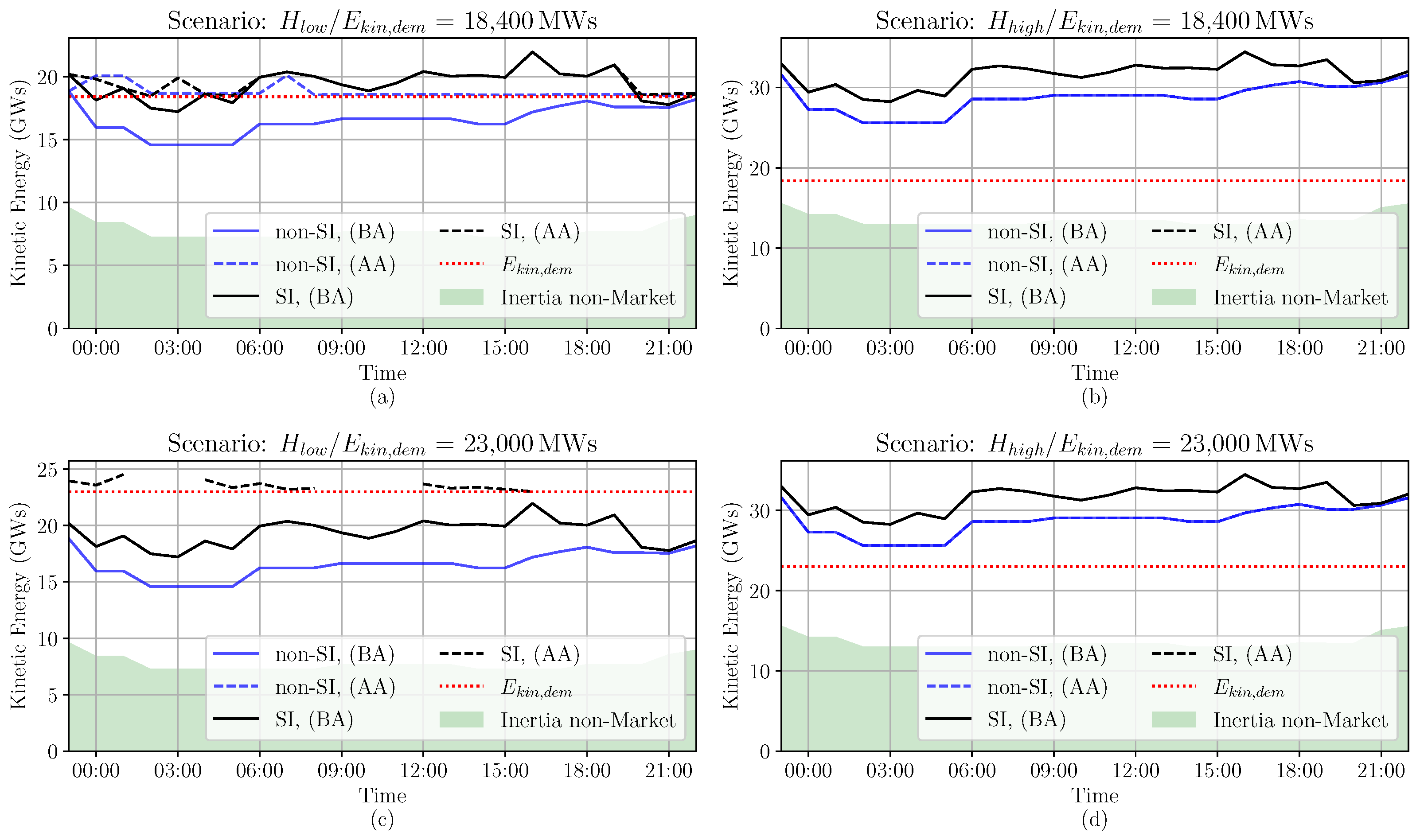
Figure 11 depict results of two days on which the inertia dispatch algorithm was applied.
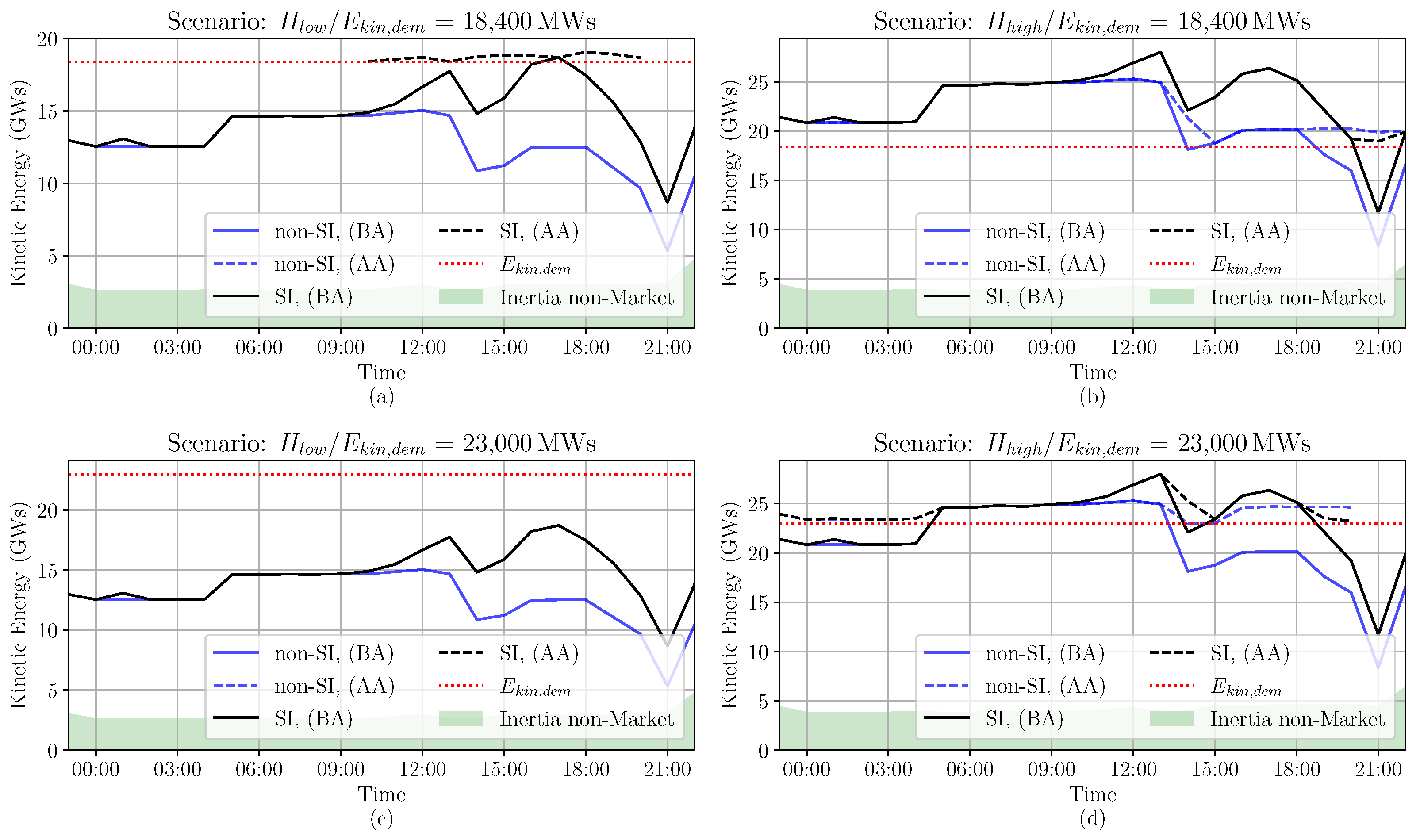
 Figure 8 and Figure 10 both depict the influence of the inertia dispatch methodology of the overall system inertia.
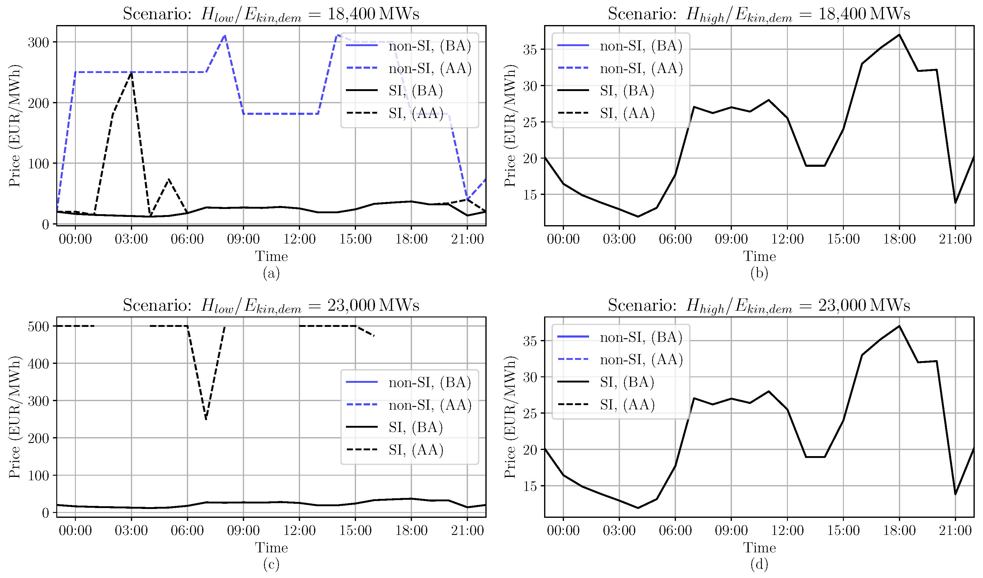
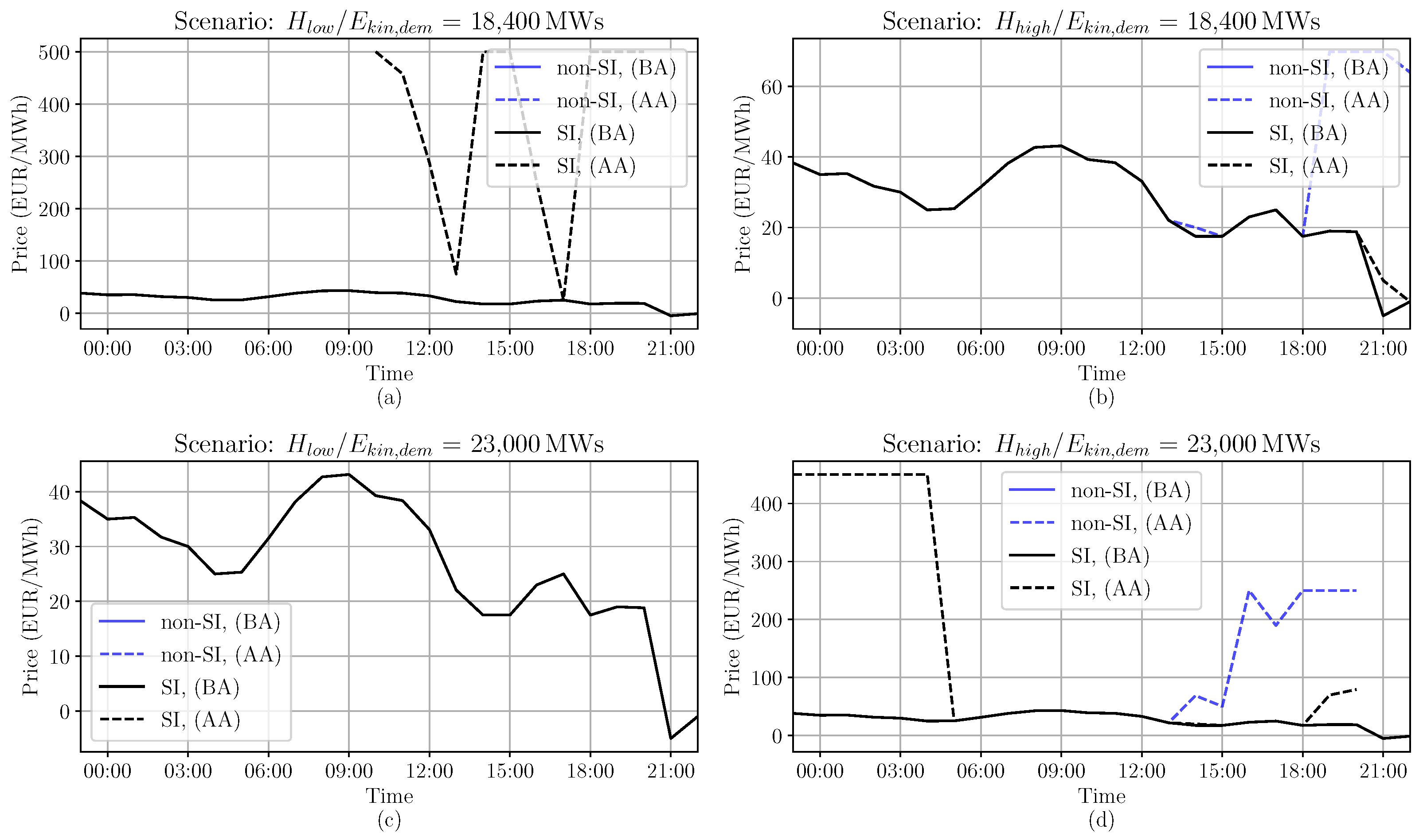
 Figure 9 and Figure 11 both depict the day-ahead market price changes due to application of the inertia dispatch algorithm. Results of a day with a higher average system kinetic energy are shown in Figure 8 and for the price in Figure 9, whereas a day with lower average kinetic energy is shown in Figure 10 and the price for the same day in Figure 11. Each subplot of the Figures shows a different combination of E k i n , d e m and the assumption of the generators inertia constant ( H l o w or H h i g h ). The blue line depicts the scenario where SI by WT is not considered and the black line where SI by WT is integrated. The solid line illustrates the result before application (BA) of the inertia dispatch algorithm and the dotted blue line the result after application (AA) of the algorithm. The green area in Figure 8 and Figure 10 within each subplot, depicts the stored kinetic energy provided by units which are not trading on the day-ahead market and the red dotted line the demanded system kinetic energy.
The subplots in Figure 8 show the resulting stored system kinetic energy over time for one day, in this case the 2020-06-11. The top left subplot depicts the results for the combination E k i n , d e m = 18,400 MWs and H l o w . The positive contribution of inertia supplying WT is clearly visible. As the blue line (no SI contribution) is almost steadily below the demanded system kinetic energy, the black line (SI contribution) is above the red dotted line, especially from 5:00 to 19:00. After application of the dispatch algorithm sufficient stored kinetic energy can be achieved for the whole day. This is represented by both dotted lines being above the demanded kinetic energy (red line). The price illustration for the same day and combination is depicted in the top left subplot of Figure 9. If no SI is provided by WT significantly more inertia needs to be supplied by synchronous generators which is visible by higher prices. As by nature of the inertia dispatch algorithm, the merit order is restructured and synchronous generators are included as long as kinetic energy is needed. The newly added synchronous generator sets the market balance price which is obviously higher, most likely due to higher marginal prices. Price changes when inertia is provided by WT is not as significant. The bottom left subplot of Figure 8 shows results of the combination E k i n , d e m = 23,000 MWs and H l o w . Without applying the inertia dispatch algorithm, the system kinetic energy is below E k i n , d e m all day. Applying the inertia dispatch algorithm when inertia is provided by WT, during some hours of the day, the requirement for sufficient system kinetic energy is achieved by the algorithm (see dotted black line). Non-existing parts of the dotted black line indicates that no solution could be achieved by the algorithm. The power price during the hours where the inertia algorithm is successful, is in this scenario indicated by high prices of 500 EUR/MWh. For both remaining subplots in Figure 8 (top right and bottom right subplot) both combinations result in sufficient stored system kinetic energy for the whole day. Hence, the algorithm is not executed and the power price does not change as visible in the top right and bottom right subplot in Figure 9.
Figure 10 and Figure 11 show the results for the 2020-04-12. A day which is characterised by less system inertia compared to the previously explained scenario results. For every combination the inertia dispatch algorithm had to be executed as visible by the dotted lines in the subplots in Figure 10. No solution was found by the algorithm for the scenario E k i n , d e m = 23,000 MWs and H l o w as visible in the bottom left subplot. Again, it is visible that SI of WT is able to provide a significant amount of kinetic energy to the overall system kinetic energy. This is particularly during the second half of the day. Figure 11 shows the power price changes due to insufficient inertia. In some hours the price increases significantly. See top left subplot at 10:00, 14:00, 15:00 and hours from 18:00 onward and the first hours of the day until 04:00 in the bottom right subplot. As no solution was found by the algorithm for the combination E k i n , d e m = 23,000 MWs and H l o w (bottom left subplot), only the power prices before application of the algorithm are illustrated.
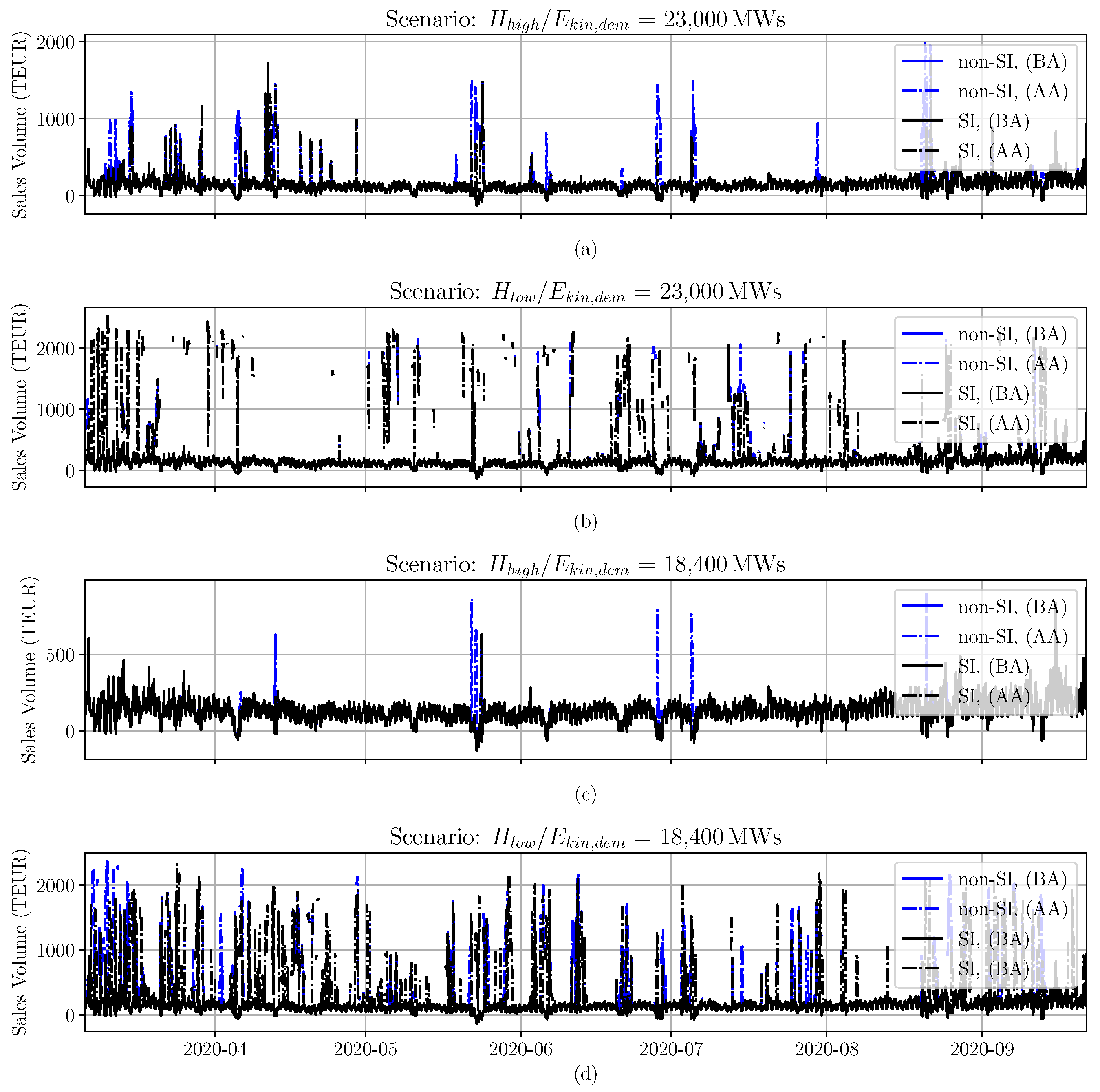
Figure 12 shows the sales volume over time for each trading period of the analysed time series. The sales volume for each trading period is calculated by multiplying the traded volume and the power market price. Figure 12 is split into four subplots. Each of the four subplots shows a combination possibility of E k i n , d e m = 18,400 MWs, E k i n , d e m = 23,000 MWs, H l o w and H h i g h . A single subplot depicts the sales volume with (black graph) and without (blue graph) SI provided by WT before (BA) and after application (AA) of the algorithm. For each combination, the sales volume is in the range of 0 TEUR to 2500 TEUR. The combination E k i n , d e m = 18,400 MWs and H h i g h leads to the scenario were the algorithm is activated the least times compared to the other scenarios, whereas the combinations E k i n , d e m = 18,400 MWs and H l o w leads to the highest times of algorithm activation. Further, the y-axis labels for the combination E k i n , d e m = 18,400 MWs and H h i g h ranges only from 0 TEUR to 750 TEUR.
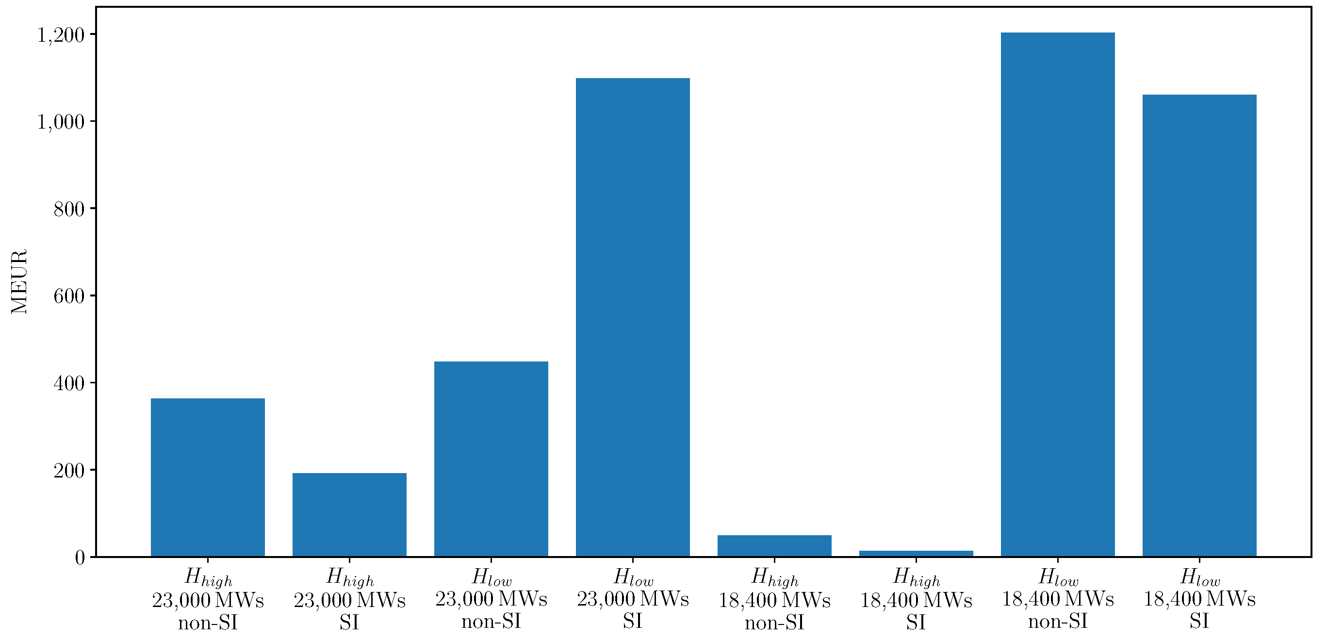
Figure 13 shows the accumulated sums of the sales volume for each scenario. Each bar illustrates a single scenario. Except for the scenario E k i n , d e m = 23,000 MWs and H l o w the positive influence of SI from WT on the overall lower sales volume is visible. The overall sales volume if SI is provided by WT is, except for one combination, significantly lower. The likely explanation for the one exception is the the high number of times where the algorithm was not able to find a solution to meet the condition of sufficient system kinetic energy. Visible as well, is the fact that the assumption of higher generator inertia constants leads to fewer activation of the algorithm and hence to lower total sales volumes.
It is already determined that the future trading unit for the commodity inertia should be EUR/kgm2 (or any other currency), whereas kgm2 is the unit of the moment of inertia (J) of a synchronously connected machine [2]. By rearranging
E k i n , s y s = 1 2 J s y s · ( 2 π f g r i d , n o m ) 2
where E k i n , s y s is the system-wide stored kinetic energy, J s y s being the overall moment of inertia and f g r i d , n o m is the nominal grid frequency of 50 Hz as in the case of the AC power system of Ireland, the overall moment of inertia can be calculated to assess the additional costs for the additionally supplied inertia. The fourth column of Table 3 shows the calculated results, which represent average values for the researched time period. With respect to the additionally supplied inertia, the costs for inertia range from 1.02 EUR/kgm2 to 4.49 EUR/kgm2. The calculated results are in the same order of magnitude as previous research indicate [2].

5. Discussion

To secure power system stability, the Irish TSO has defined objectives of various operational constraints, one being the operational limit for inertia [26]. Based thereon is the research presented in the work at hand. Comparing the results presented in Table 3 and the times where the inertia dispatch algorithm is applied and the All Island Quarterly Wind Dispatch Down Report 2020 (Qtr. 3) there is a obvious abnormality [9]. The published statistics [9] indicate the dispatched down energy by WT listed for each curtailment category for each month. Table 3 lists the absolute number of times the inertia dispatch methodology is applied for the different combinations. Even though the numbers are not directly comparable, it is obvious that the dispatch algorithm tends to overestimate the times of insufficient inertia in the power system.
One explanation is that the research was carried out with only publicly available data. The TSO and the market operators publish various information. Still, the results indicate that not all information which would lift the amount of stored kinetic energy in the power system up are obtainable. For example, power plants connected to the power system but only used for self consumption—e.g., the case of steel mills. Small units not trading on the market and connected to the distribution grid are not listed by the transparency platform of the ENTSO-E. Though, if equipped with a synchronous generator, the units contribute to the overall power system inertia. Second, the assumed inertia constant per fuel type (Table 2) is crucial to estimating the overall power system inertia. Table 3 indicates a huge gap comparing the scenarios applying H l o w and the scenarios applying H h i g h . The times where the dispatch methodology was applied increased significantly when the lower inertia constant bound ( H l o w ) was used. It is safe to assume that the scenarios applying the lower bound of the inertia constant range ( h l o w ) underestimate the power system inertia constant clearly. Hence, it can be assumed that the actual inertia constant of the Irish generation units is close to the upper bound values or even above. The same pattern, as described before, is visible, where the application of the methodology results in no solution. The results of the scenarios with the H l o w assumptions are rather unreasonable.
Figure 9 and Figure 11 illustrate a pattern which is visible throughout most of the results. Even a marginal increase of the power system inertia, due to the restructuring of the merit order by the inertia dispatch algorithm, results in significant price increases up to 250 EUR/MWh and beyond. It can be assumed that applying the inertia dispatch algorithm in reality, the biding structure of power plant operators would change. More power plant operators would tend to bid, as due to the possibility of low power system inertia and the perspective of the application of the inertia dispatch algorithm, their bids would be accepted. This scenario is likely to result in more power selling bids and lower price bids. Unfortunately, this cannot be simulated in this study, as the research at hand relies on actual power market data and no generic literature cost data is used. The bidding behavior of market participants under new market rules is not within the focus of this work.
A new bidding behavior of market participants would also decrease the number of times the algorithm would not be able to find a solution. Finding no solution to the problem formulation is obviously worst of all outcomes as the problem of insufficient power system inertia remains to be solved by the TSO. Hence, the TSO has to activate other sources providing inertia—for example, decommissioned power plants, which are most likely decommissioned for safety or economical reasons, which ultimately increase overall system costs; or storage units providing inertia, such as flywheels. Previous research indicates that storage units solely used for the provision of inertia are vastly expensive [2]. Comparing the costs for additional inertia from Table 3 with results from [2] shows that the application of the dispatch methodology and temporarily price increases are overall less expensive than securing sufficient inertia by storage unit solutions. Still, a single market for power system inertia has to be developed and should decreases costs for inertia in power systems [33].

6. Conclusions

This study applied and assessed a novel dispatch methodology of the day-ahead market to secure sufficient inertia in power systems and researched the influence of SI provided by WT on power prices. The methodology allows to determine costs per additionally supplied inertia. This work applied actual data provided by the day-ahead market operator of the combined power market of the Republic of Ireland and Northern Ireland, and data from the TSO and the ENSTO-E. Eight scenarios were designed which cover different inertia constants per fuel type, two operation limits of stored kinetic energy and the application of SI provided by WT.
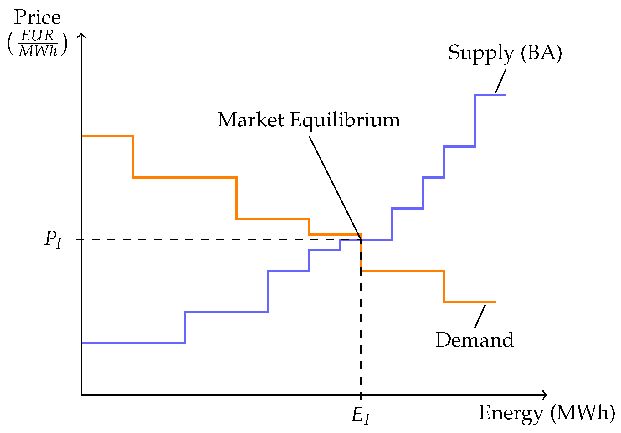
If basic market operation without application of the inertia market methodology results in an insufficient level of stored kinetic energy, the arranged sell bids of the day-ahead market are restructured. With respect to the researched scenario, SI is either part of the process or is not. In decreasing price order, sell bids of units not providing inertia get replaced by the following unit in the merit order. This iterative process is repeated until a level of sufficient inertia is achieved, and then it continues in the next trading period. Trading periods where a sufficient amount of kinetic energy cannot be realised by the algorithm occur.
Overall, a six month period with a total of 4799 trading periods was researched. Based on the combination, the results differ significantly and the prices on the day-ahead market increase significantly too. Applying SI provided by WT decreases costs and the number of times the inertia dispatch methodology is applied. Naturally, a scenario with a lower operational limit for inertia, higher assumed inertia constants for generation units and inertia support from WT, results in fewer applications of the inertia dispatch algorithm and lower costs for the additionally supplied inertia, compared to a scenario with a higher operational limit for inertia and/or lower assumptions of inertia constants for different generation units. The average cost per additionally supplied inertia ranges from 1.02 to 4.49 EUR/kgm2.
The inertia dispatch methodology assessed in this work is a useful approach with which to secure a sufficient amount of inertia in power systems. However, it has limitations, and the results clearly indicate that the provision of power system inertia in future power systems has to be decoupled from the power market, because market prices resulting from the inertia dispatch algorithm are too high. Future research has to assess whether a single market for trading inertia is capable of providing sufficient inertia to secure grid frequency controllability at reasonable system costs [2,33]. Similar to markets for primary frequency control (where power is traded) or capacity markets, the provision of inertia for a certain time period would be traded, rather than the actual utilisation of the system’s service inertia [2]. As inertia is a non-traded commodity and its costs have so far been researched only superficially, the results determined in this work can be seen as an indicator for future prices on such a market for the provision of inertia.

Author Contributions

H.T. performed the research and wrote the paper. C.J. conceived the basic idea of the paper, reviewed the paper and contributed with valuable discussion and supervision. All authors have read and agreed to the published version of the manuscript.

Funding

This research received no external funding.

Conflicts of Interest

The authors declare no conflict of interest.

Abbreviations

The following abbreviations are used in this manuscript:
ROCOFrate of change of frequency
SIsynthetic inertia
TSOtransmission system operator
WTwind turbines

References

  1. Tielens, P.; Hertem, D.V. The relevance of inertia in power systems. Renew. Sustain. Energy Rev. 2016, 55, 999–1009. [Google Scholar] [CrossRef]
  2. Thiesen, H.; Jauch, C.; Gloe, A. Design of a System Substituting Today’s Inherent Inertia in the European Continental Synchronous Area. Energies 2016, 9, 582. [Google Scholar] [CrossRef] [Green Version]
  3. Kundur, P.; Balu, N.; Lauby, M. Power System Stability and Control; EPRI Power System Engineering Series; McGraw-Hill: New York, NY, USA, 1994; ISBN 978-0-07-035958-1. [Google Scholar]
  4. Bian, Y.; Wyman-Pain, H.; Li, F.; Bhakar, R.; Mishra, S.; Padhy, N.P. Demand Side Contributions for System Inertia in the GB Power System. IEEE Trans. Power Syst. 2018, 33, 3521–3530. [Google Scholar] [CrossRef]
  5. Ruttledge, L.; Miller, N.; O’Sullivan, J.; Flynn, D. Frequency Response of Power Systems With Variable Speed Wind Turbines. IEEE Trans. Sustain. Energy 2013, 3, 683–691. [Google Scholar] [CrossRef]
  6. Gloe, A.; Jauch, C.; Craciun, B.; Winkelmann, J. Continuous provision of synthetic inertia with wind turbines: Implications for the wind turbine and for the grid. IET Renew. Power Gener. 2019, 13, 668–675. [Google Scholar] [CrossRef]
  7. Hydro Québec TransÉnergie. Technical Requirements for the Connection of Generation Facilities to the Hydro-Québec Transmission System. Supplementary Requirements for Wind Generation. 2005. Available online: https://www.aeeolica.org/uploads/documents/4535-separata-del-borrador-de-po122.pdf (accessed on 25 May 2020).
  8. EirGrid. Annual Renewable Energy Constraint and Curtailment Report 2019. 2020. Available online: http://www.eirgridgroup.com/site-files/library/EirGrid/Annual-Renewable-Constraint-and-Curtailment-Report-2019-V1.2.pdf (accessed on 10 December 2020).
  9. EirGrid. All Island Quarterly Wind Dispatch Down Report. 2020. Available online: http://www.eirgridgroup.com/site-files/library/EirGrid/Grid-Code.pdf (accessed on 25 May 2020).
  10. Thiesen, H.; Jauch, C. A dispatch methodology to secure power system inertia in future power systems. In Proceedings of the 17th International Workshop on Large-Scale Integration of Wind Power into Power Systems as Well as on Transmission Networks for Offshore Wind Power Plants (Energynautics GmbH), Stockholm, Sweden, 17–19 October 2018. [Google Scholar]
  11. O’Sullivan, J.W.; O’Malley, M.J. A new methodology for the provision of reserve in an isolated power system. IEEE Trans. Power Syst. 1999, 14, 519–524. [Google Scholar] [CrossRef]
  12. Doherty, R.; Lalor, G.; O’Malley, M. Frequency control in competitive electricity market dispatch. IEEE Trans. Power Syst. 2005, 20, 1588–1596. [Google Scholar] [CrossRef]
  13. Lee, Y.-Y.; Baldick, R. A frequency-constrained stochastic economic dispatch model. IEEE Trans. Power Syst. 2013, 28, 2301–2312. [Google Scholar] [CrossRef]
  14. Daly, P.; Flynn, D.; Cunniffe, N. Inertia considerations within unit commitment and economic dispatch for systems with high non-synchronous penetrations. In Proceedings of the 2015 IEEE Eindhoven PowerTech, Eindhoven, The Netherlands, 29 June–2 July 2015; pp. 1–6. [Google Scholar] [CrossRef] [Green Version]
  15. Teng, F.; Trovato, V.; Strbac, G. Stochastic Scheduling With Inertia-Dependent Fast Frequency Response Requirements. IEEE Trans. Power Syst. 2016, 31, 1557–1566. [Google Scholar] [CrossRef] [Green Version]
  16. Collins, S.; Deane, J.P.; Ó Gallachóir, B. Adding value to EU energy policy analysis using a multi-model approach with an EU-28 electricity dispatch model. Energy 2017, 130, 433–447. [Google Scholar] [CrossRef]
  17. Johnson, S.C.; Papageorgiou, D.J.; Mallapragada, D.S.; Deetjen, T.A.; Rhodes, J.D.; Webber, M.E. Evaluating rotational inertia as a component of grid reliability with high penetrations of variable renewable energy. Energy 2019, 180, 258–271. [Google Scholar] [CrossRef]
  18. Zhang, Z.; Wang, Y.; Li, H.; Su, X. Comparison of inertia control methods for DFIG-based wind turbines. In Proceedings of the 2013 IEEE ECCE Asia Downunder, Melbourne, VIC, Australia, 3–6 June 2013; pp. 960–964. [Google Scholar] [CrossRef]
  19. The Single Electricity Market Operator (SEMO). List of Registered Units-April. 2020. Available online: https://www.sem-o.com/documents/general-publications/List-of-Registered-Units.xlsx (accessed on 25 May 2020).
  20. The Single Electricity Market Operator (SEMO). Market Parameters. 2020. Available online: https://www.sem-o.com/documents/market-parameters/1819-IE-CLAF-Publication-v6.0.pdf (accessed on 12 November 2020).
  21. Met Éireann. Historical Data. 2020. Available online: https://www.met.ie/climate/available-data/historical-data (accessed on 12 November 2020).
  22. Jonkman, J.; Butterfield, S.; Musial, W.; Scott, G. Definition of a 5MW Reference Wind Turbine for Offshore System Development; National Renewable Energy Lab. (NREL): Golden, CO, USA, 2009. [Google Scholar] [CrossRef] [Green Version]
  23. SEMOpx. Market Data. 2020. Available online: https://www.semopx.com/market-data/ (accessed on 24 May 2020).
  24. SEMOpx. SEMOpx Operating Procedures: DAM, IDA, IDC. 2019. Available online: https://www.semopx.com/rules-and-monitoring/market-rules/SEMOpx-Operating-Procedures.docx (accessed on 20 April 2020).
  25. ENTSO-E. ENTSO-E Transparency Platform. 2020. Available online: https://transparency.entsoe.eu/ (accessed on 15 November 2020).
  26. EirGrid and SONI. Operational Constraints Update 31/01/2020. 2020. Available online: http://www.eirgrid.ie/site-files/library/EirGrid/OperationalConstraintsUpdateVersion1_90_January_2020.pdf (accessed on 24 May 2020).
  27. Machowski, J.; Lubosny, Z.; Bialek, J.; Bumby, J. Power System Dynamics: Stability and Control, 2nd ed.; Wiley: West Sussex, UK, 2020; ISBN 978-1-119-52638-4. [Google Scholar]
  28. Ørum, E.; Kuivaniemi, M.; Laasonen, M.; Bruseth, A.I.; Jansson, E.A.; Danell, A.; Elkington, K.; Modig, N. Nordic Report-Future System Inertia. 2015. Available online: https://www.statnett.no/globalassets/for-aktorer-i-kraftsystemet/utvikling-av-kraftsystemet/nordisk-frekvensstabilitet/future-system-inertia-phase-1.pdf (accessed on 27 July 2018).
  29. Seneviratne, C.; Ozansoy, C. Frequency response due to a large generator loss with the increasing penetration of wind/PV generation-A literature review. Renew. Sustain. Energy Rev. 2016, 57, 659–668. [Google Scholar] [CrossRef]
  30. Pfenninger, S.; DeCarolis, J.; Hirth, L.; Quoilin, S.; Staffell, I. The importance of open data and software: Is energy research lagging behind? Energy Policy 2017, 101, 211–215. [Google Scholar] [CrossRef]
  31. Thiesen, H. Github Inertia Dispatch. 2020. Available online: https://github.com/hnnngt/inertia_dispatch (accessed on 27 May 2020).
  32. Thiesen, H.; Jauch, C. Determining the load inertia contribution from different power consumer groups. Energies 2020, 13, 1588. [Google Scholar] [CrossRef] [Green Version]
  33. ENTSO-E. Need for Synthetic Inertia (SI) for Frequency Regulation. 2017. Available online: https://www.entsoe.eu/Documents/Network%20codes%20documents/Implementation/CNC/IGD-Need_for_Synthetic_Inertia.pdf (accessed on 29 March 2017).
Figure 1. Characteristics of the variable H controller [6].
Energies 14 01255 g001
Figure 2. Simplified flow chart of the day-ahead market including the dispatch methodology to supply sufficient power system inertia (based on [10]). The dotted line, marking the inertia dispatch algorithm, cuts the supply box in half, symbolising the algorithm’s influence on the merit order.
Energies 14 01255 g002
Figure 3. Intersection of the supply (blue) and demand (orange) graph before application (BA) of the inertia dispatch algorithm.
Energies 14 01255 g003
Figure 4. Intersection of the supply (blue) and demand (orange) graph before application (BA) of the inertia dispatch algorithm, and the demand graph (green) after application (AA) of the inertia dispatch algorithm.
Energies 14 01255 g004
Figure 5. Methodology illustrating how the potential available inertia of the WT is calculated.
Energies 14 01255 g005
Figure 6. Power curve of the NREL 5 MW WT [22].
Energies 14 01255 g006
Figure 7. Power vs. rotational speed characteristic [22].
Energies 14 01255 g007
Figure 8. Algorithm results of 2020-06-11. (a) Scenario: low operational limit of kinetic energy and low inertia constants per fuel type, (b) Scenario: low operational limit of kinetic energy and high inertia constants per fuel type, (c) Scenario: high operational limit of kinetic energy and low inertia constants per fuel type, (d) Scenario: high operational limit of kinetic energy and high inertia constants per fuel type. Each subplot depicts the overall system-wide stored kinetic energy with (black graph) and without (blue graph) system inertia by WT before (BA) and after application (AA) of the inertia dispatch methodology. The green area depicts the stored kinetic energy of units which are not traded on the day-ahead market.
Energies 14 01255 g008
Figure 9. Algorithm results of the 2020-06-11. (a) Scenario: low operational limit of kinetic energy and low inertia constants per fuel type, (b) Scenario: low operational limit of kinetic energy and high inertia constants per fuel type, (c) Scenario: high operational limit of kinetic energy and low inertia constants per fuel type, (d) Scenario: high operational limit of kinetic energy and high inertia constants per fuel type. Each subplot illustrates the market price with (black graph) and without (blue graph) system inertia by WT before (BA) and after application (AA) of the inertia dispatch methodology.
Energies 14 01255 g009
Figure 10. Algorithm results of the 2020-04-12. (a) Scenario: low operational limit of kinetic energy and low inertia constants per fuel type, (b) Scenario: low operational limit of kinetic energy and high inertia constants per fuel type, (c) Scenario: high operational limit of kinetic energy and low inertia constants per fuel type, (d) Scenario: high operational limit of kinetic energy and high inertia constants per fuel type. Each subplot depicts the overall system-wide stored kinetic energy with (black graph) and without (blue graph) system inertia by WT before (BA) and after application (AA) of the inertia dispatch methodology. The green area depicts the stored kinetic energy of units which are not traded on the day-ahead market.
Energies 14 01255 g010
Figure 11. Algorithm results of the 2020-04-12. (a) Scenario: low operational limit of kinetic energy and low inertia constants per fuel type, (b) Scenario: low operational limit of kinetic energy and high inertia constants per fuel type, (c) Scenario: high operational limit of kinetic energy and low inertia constants per fuel type, (d) Scenario: high operational limit of kinetic energy and high inertia constants per fuel type. Each subplot illustrates the market price with (black graph) and without (blue graph) system inertia by WT before (BA) and after application (AA) of the inertia dispatch methodology.
Energies 14 01255 g011
Figure 12. Sales volume over time before and after application of the methodology. (a) Scenario: high operational limit of kinetic energy and high inertia constants per fuel type, (b) Scenario: high operational limit of kinetic energy and low inertia constants per fuel type, (c) Scenario: low operational limit of kinetic energy and high inertia constants per fuel type, (d) Scenario: low operational limit of kinetic energy and low inertia constants per fuel type.
Energies 14 01255 g012
Figure 13. Total sales volume after application of the methodology. Each bar depicts a different scenario combination.
Energies 14 01255 g013
Table 1. Overview of the applied data and information.
DataContent/DescriptionSources
WT H v a r CharacteristicsData to determine H v a r [6]
List of Registered UnitsList containing Resource name, installed capacity, fuel type[19]
WT LocationList of WT locations per county[20]
Historical Wind Speed DataWind speed data in hourly resolution[21]
NREL 5 MW DataPower curve & power vs. Speed characteristic[22]
Day-Ahead Market DataSell and buy bids per trading period[23]
Exchange RatesPound Sterling-Euro exchange rates[24]
ENTSO-E Generation DataGeneration data of units not trading on day-ahead market[25]
System Operational ConstraintsInformation regarding demanded kinetic energy[26]
Table 2. Inertia constants for different power generation types.
Fuel Type H l o w (s) H h i g h (s)Sources
Biomass2-[27]
Coal44.25[27,28]
Distillate3.5-[27]
Gas3.56.25[27,29]
Hydro14.5[28,29]
Oil3.5-[27]
Peat3.7-[27]
Pump Storage5.56.35[27,29]
Table 3. Methodology results.
ScenarioTimes of Methodology ApplicationTimes of No SolutionCosts for Additional Inertia (EUR/kgm2)
E k i n , d e m = 23,000 MWs, H h i g h , non-SI789384.49
E k i n , d e m = 23,000 MWs, H h i g h , SI50753.98
E k i n , d e m = 18,400 MWs, H h i g h , non-SI30601.7
E k i n , d e m = 18,400 MWs, H h i g h , SI13301.02
E k i n , d e m = 23,000 MWs, H l o w , non-SI46834129-
E k i n , d e m = 23,000 MWs, H l o w , SI45733591-
E k i n , d e m = 18,400 MWs, H l o w , non-SI31631358-
E k i n , d e m = 18,400 MWs, H l o w , SI2547896-
Publisher’s Note: MDPI stays neutral with regard to jurisdictional claims in published maps and institutional affiliations.

