Evaluation of Medium Voltage Network for Propagation of Supraharmonics Resonance

Abstract

Power converters with high switching frequency used to integrate renewable power sources to medium and low voltage networks are sources of emission in the supraharmonic range (2 to 150 kHz). When such converters are connected to a medium voltage (MV) network these supraharmonics propagate through the MV network and can impact network and customer equipment over a wide range. This paper evaluates an existing Swedish MV electrical network and studies the pattern of supraharmonic resonance and the propagation of supraharmonics. The MV network consists of eight feeders including a small wind farm. Simulations reveal that, the bigger the MV network, the more resonant frequencies, but also the lower the amplitude of the resonance peaks in the driving point impedance. It was also identified that for short feeders as length increases, the magnitude of the transfer impedance at supraharmonic frequency decreases. For further increment in feeder length, the magnitude increases or becomes almost constant. For very long feeders, the transfer impedance further starts decreasing. The eight feeders in the network under study are similar but show completely different impedance versus frequency characteristics. Measurements at the MV side of the wind farm show time varying emissions in the supraharmonic range during low power production. The impact of these emissions coupled with system resonance is examined.

1. Introduction

The integration of renewable energy sources, such as solar photovoltaic installations and wind turbines, to the modern electric grid using static power converters results in the emission of supraharmonics (frequency components in the range between 2 kHz and 150 kHz). This range of frequency has gained significant attention, due to the increasing amount of equipment with active switching emitting supraharmonics. Lack of knowledge has been identified on aggregation, propagation and amplification of supraharmonic disturbances [1], and on research to extend the standard framework for power quality to supraharmonics [2]. Standardization organizations such as IEC (SC 77A), CENELEC (SC 205A) and IEEE are actively involved in developing standards that cover this frequency range.

Increased levels of supraharmonics have a number of adverse consequences, including malfunctioning and failure of control circuits and protection devices, impact on light intensity of LED lamps [3,4], insulation failures in cables [5], heating and accelerated aging of capacitor banks [6], heating and accelerated aging of transformers and rotating machines and loss of power line communication with smart meters [7].

A number of studies report the propagation of emission in the low voltage (LV) distribution grid [3,8,9,10,11]. A study on multiple device malfunction and noise in household appliances due to supraharmonic emissions in a public low voltage grid connected to a CNC mill with power converter is reported in [11]. Some of the emission from various LV sources may reach the MV grid, although generally the supraharmonic emission remain within the low-voltage installation [1,9]. Further studies have also verified that supraharmonic distortion typically decreases when propagating from a load towards the upstream network [12]. Some studies have addressed or at least mentioned resonances in LV networks at supraharmonic frequencies [13,14,15], but no such studies are carried out in the MV network.

Renewable energy-based power plants are a dominant source of supraharmonics in MV networks [16,17,18]. Grid connected solar power plants and small wind power plants are connected to the distribution network through PWM controlled power converters. They inject harmonics and supraharmonics at the point of common coupling while injecting active and reactive power to the existing network [19]. Static power converter used in variable speed control of wind turbine generators is a source of supraharmonics. Some of the different techniques adapted to improve the power quality of the grid are also sources of supraharmonics. The voltage-source converters used in FACTS devices having switching frequencies in the kHz range are sources of supraharmonics [20,21]. References [22,23] present measurement data identifying the sources of supraharmonics and their propagation through the MV network. The emission from sources connected to the MV network will spread through the MV network and from there to equipment connected to the LV grid. Equipment connected to the LV and MV network and components in the MV network may be damaged or otherwise negatively impacted by the supraharmonics. A detailed study on the characteristics of MV network for propagation of high frequency emissions are missing in literature and it has become a topic of growing interest within the power quality research group.

The case study of the Eagle Pass HVDC connection confirmed the failure of MV cable terminations due to a local resonance at 12.4 kHz triggered by a supraharmonic component [5,24]. To quantify the impact of supraharmonics, indices are proposed for MV cable termination failure [25], audible noise, light flicker and tripping of the residual current breaker [26].

Understanding the origin of supraharmonics at the terminals of sensitive equipment or grid components requires information on the source (emission) of the supraharmonics and their propagation. The driving-point impedance and transfer impedances play an important role in this propagation. Resonances play an important role here as well; high harmonic levels are often associated with resonances. The measurement of supraharmonics propagation in a large MV network with multiple feeders is challenging as it requires instrument transformers with high frequency response. The other challenge in the MV network is to distinguish primary and secondary emission. Apart from this the uncertainty of the number of supraharmonic sources such as PV plant, wind plant, industrial drives to be connected to the MV network in the near future is also a major concern. Hence the study of transfer impedance of a MV network for high frequency emissions is the need of the hour. This paper studies the resonance frequency of the MV network with eight feeders using MATLAB modelling. Further it determines the transfer impedance by injecting a supraharmonic component obtained from measurements at the wind farm in one of the feeders into the MATLAB model with all eight feeders and analyzing the results.

This paper studies the propagation of supraharmonics through the MV network. Section 2 of this paper presents the supraharmonic propagation in MV network and describe the circuit under study. Section 3 describes the distributed parameter transmission line model. The analysis in Section 4 reveals the characteristics of the feeders. Real-time measurements are evaluated for supraharmonics emissions in Section 5 and a further estimation of the transfer impedance of the MV network by injecting supraharmonic emission into the MATLAB model is given in Section 6, followed by the conclusions in Section 7.

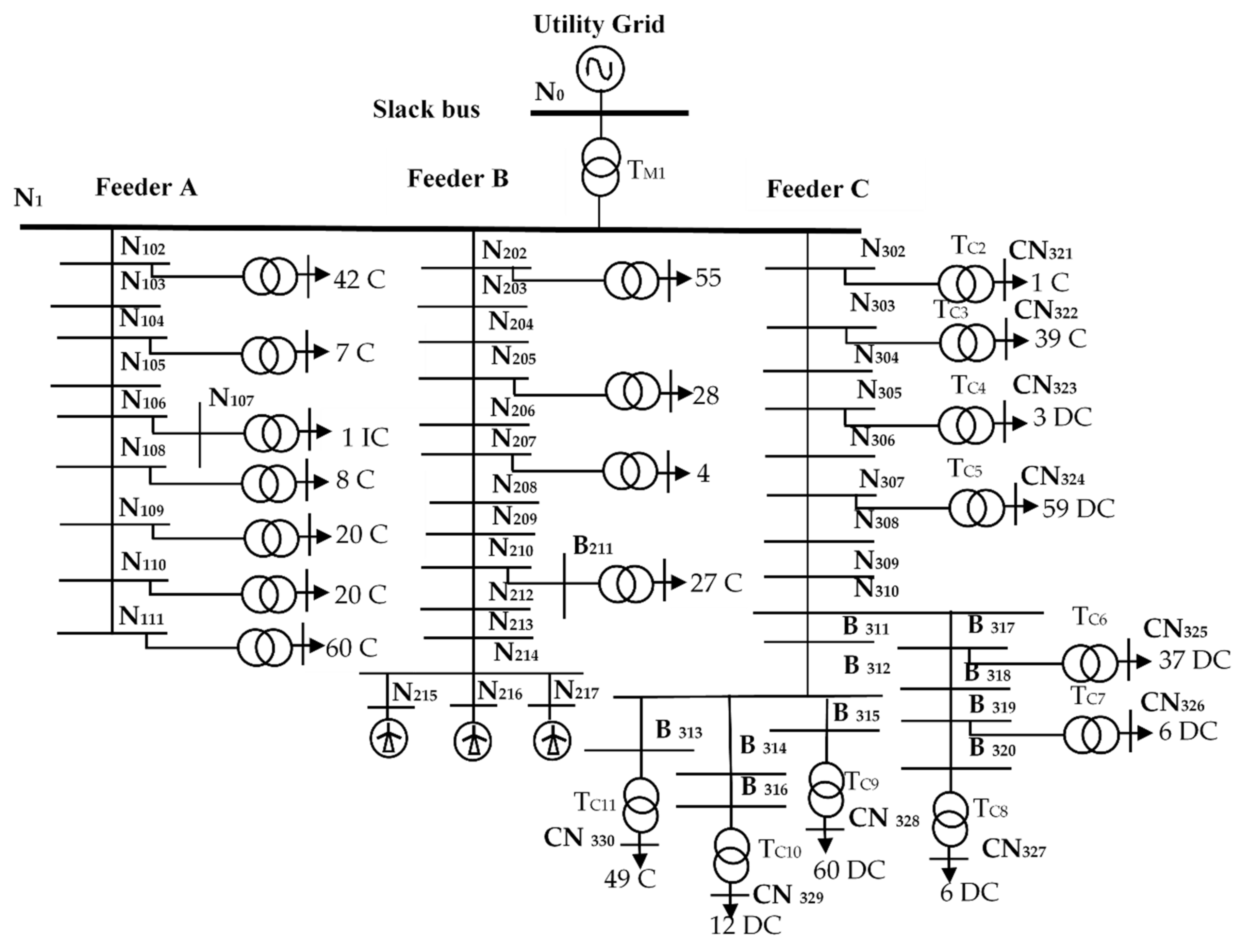
2. Case Study: Supraharmonic Propagation in MV Network

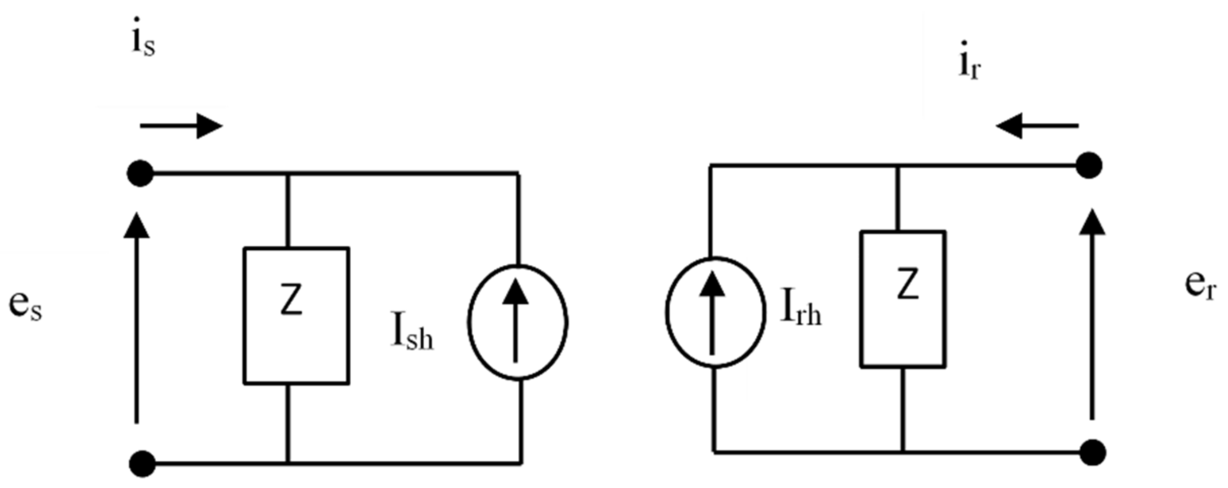
The harmonic distortions generated by power-electronic converters, coupled with system resonance, can cumulatively intensify when damping is insufficient and this may severely affect the system operation. The impedance variation and the resulting system resonance depends upon factors such as the cable length, short circuit power of the system, VAR compensator with harmonic filter and the load level in the system [22]. Reference [22] analyzed the propagation of supraharmonics in a 20 kV electrical network with MV wind-power plants and LV/MV solar-power plants. A very strong correlation was observed between supraharmonics measured at two substations 16 km apart. This showed the possibility of propagation of supraharmonics over long distances. The investigators also monitored voltage and current of 119th harmonic for 24 h and found that the levels were significantly higher between sunrise and sunset.

From the measurements, [23] concluded that solar power plants cause voltage distortion in the range between 3 and 6 kHz as their values are above background distortion level between sunrise and sunset. Correlations in time behavior around 2.5 kHz identified a wind power plant as the source for those frequencies.

To study the propagation of supraharmonics, an existing Swedish MV rural network (underground cabling) with eight feeders and three wind turbines in feeder B has been modelled in detail using simscape power systems toolbox in MATLAB/SIMULINK. The distributed parameter transmission line model described in Section 3 had been used for underground cables. The 16 MVA, 33 kV/11 kV transformer provides service to about 2000 low-voltage and a few medium-voltage customers. The MV network consists of eight feeders with a total length of 110 km and about 115 distribution transformers.

The length of the underground cables, number of transformers and number of customers in each feeder are given in

Table 1. Feeder details.

Feeder	Length of the Cables (km)	Number of Transformers	Number of Customers
Feeder A	3.790	7	Domestic–115 Industry–1
Feeder B	6.7663	4 + 3 (Connected to Wind turbines)	Domestic–114
Feeder C	5.0894	7	Domestic–272
Feeder D	29.5824	25 + 2 (Connected to Power Station)	Domestic–313
Feeder E	4.445	8	Domestic–332
Feeder F	20.0559	18	Domestic–213
Feeder G	2.2002	6	Domestic–275
Feeder H	39.5786	33	Domestic–345

.

Table 2. 33 kV/11 kV Transformer details.

Power Rating	16 MVA
Impedance	10.5 %
Bus Voltage	11 kV	33 kV
Fault level	81.5 MVA	153.6 MVA
Source Reactance	1.68 ohms	7.76 ohms
Source Resistance	0.15 ohms	1.07 ohms

gives details for the main 33 kV/11 kV substation transformer.

3. Methodology Used

In order to determine a suitable model to study the propagation of supraharmonics, the need for distributed parameter models was estimated. The longest section in feeder C is about 400 m long. The capacitance of this section is 0.12 µF and its inductance is 0.12 mH, resulting in a resonance frequency of 30 kHz. The lumped parameter model (with 50 Hz values for inductance and capacitance) can be used up to about one quarter of this resonance frequency, some 5–10 kHz in this case. That means that it is necessary to use distributed parameter models. The Bergeron model (in time domain) is one of the options. There is also a frequency-domain model that uses a lumped-parameter PI-model with frequency dependent parameters, as for example used in [27].

A distributed parameter transmission line model has been implemented in MATLAB/SIMULINK with lumped losses based on Bergeron’s traveling wave method as used in [28]. The two-port model used is shown in Figure 1.

The surge impedance, wave propagation speed and transport delay are given by Equations (1)–(3), respectively.

$$Z_c=\sqrt{\frac{l}{c}}$$

(1)

$$v=1/\sqrt{lc}$$

(2)

$$\tau =\frac{d}{v}$$

(3)

where $l$ and $c$ are the per unit length of inductance and capacitance, $d$ is the line length and $v$ is the propagation speed.

For a lossless line the model equations are given by (4) to (9):

$$e_r\left(t\right)-Z_c{i}_r\left(t\right)=e_s\left(t-\tau \right)+Z_c{i}_s\left(t-\tau \right)$$

(4)

$$e_s\left(t\right)-Z_c{i}_s\left(t\right)=e_r\left(t-\tau \right)+Z_c{i}_r\left(t-\tau \right)$$

(5)

where

$$i_s\left(t\right)=\frac{e_s\left(t\right)}{Z}-I_{sh}\left(t\right)$$

(6)

$$i_r\left(t\right)=\frac{e_r\left(t\right)}{Z}-I_{rh}\left(t\right)$$

(7)

$$I_{sh}\left(t\right)=\frac{2}{Z_c}{e}_r\left(t-\tau \right)-I_{rh}\left(t-\tau \right)$$

(8)

$$I_{rh}\left(t\right)=\frac{2}{Z_c}{e}_s\left(t-\tau \right)-I_{sh}\left(t-\tau \right)$$

(9)

When losses are considered, the equations for $I_{sh}$ and $I_{rh}$ are adapted by lumping one fourth of the total resistance, $\frac{R}{4}$, at both ends of the connection and $\frac{R}{2}$ in the middle of the line, where $R$ is the total resistance of the cable or line connection. At higher frequencies, where the penetration depth is controlled by the skin effect, both the resistance and reactance increase with the square root of frequency. Considering this relationship, the impedance with skin effect is calculated [29].

The current sources $I_{sh}$ and $I_{rh}$, in Figure 1, are then computed as follows:

$$I_{sh}\left(t\right)=\left(\frac{1+h}{2}\right)\left(\frac{1+h}{\mathrm{Z}}{e}_r\left(t-\tau \right)-h{I}_{rh}\left(t-\tau \right)\right)+\left(\frac{1+h}{2}\right)\left(\frac{1+h}{\mathrm{Z}}{e}_s\left(t-\tau \right)-h{I}_{sh}\left(t-\tau \right)\right)$$

(10)

$$I_{rh}\left(t\right)=\left(\frac{1+h}{2}\right)\left(\frac{1+h}{\mathrm{Z}}{e}_s\left(t-\tau \right)-h{I}_{sh}\left(t-\tau \right)\right)+\left(\frac{1+h}{2}\right)\left(\frac{1+h}{\mathrm{Z}}{e}_r\left(t-\tau \right)-h{I}_{rh}\left(t-\tau \right)\right)$$

(11)

where

$$\begin{array}{c}Z=\sqrt{\frac{l}{c}}+\frac{r}{4}\\ h=\frac{\sqrt{\frac{l}{c}}-\frac{r}{4}}{\sqrt{\frac{l}{c}}+\frac{r}{4}}\\ \tau =d\sqrt{lc}\end{array}$$

where $r,l,c$ are the resistance, inductance and capacitance per unit length, respectively, and line length is represented by $d$. For a lossless line, r = 0, h = 1, and Z = $\sqrt{\frac{l}{c}}$.

4. Results and Analysis

4.1. Feeder C First Estimation

An estimation of the resonance frequency for feeder C in Figure 2 was made. The total cable length of feeder C is 5.0894 km. From Table 2 and

Table A1. Cable parameters.

Cable	Type/Specification	Zop (Ω/km)	L (H/km)	Bsh (µS/km)	C(F/km)
C1	ACJJ/150	0.206 + 0.0754i	2.4001 × 10−4	188.5	0.6 × 10−6
C2	AXCEL/150	0.206 + 0.0911i	2.9 × 10−4	94.248	0.3 × 10−6
C3	AXCL-OTT3x150/25	0.206 + 0.0942i	2.9985 × 10−4	94.248	0.3 × 10−6
C4	AXKJ/50/16	0.641 + 0.1257i	4 × 10−4	62.832	0.2 × 10−6
C5	FXKJ/35	0.493 + 0.1068i	3.3995 × 10−4	94.248	0.3 × 10−6
C6	AXCL-OTT3x95/16	0.32 + 0.1005i	3.1990 × 10−4	94.248	0.3 × 10−6
C7	AXCEL/95	0.32 + 0.0974i	3.1003 × 10−4	94.248	0.3 × 10−6
C8	AXCEL/50	0.641 + 0.1068i	3.3995 × 10−4	94.248	0.3 × 10−6

in Appendix A the total capacitance of feeder C is 2.5208 $\mathsf{\mu }$F.

Considering only the source impedance at 33 kV and the 33 kV/11 kV transformer impedance for the inductance, the first resonance frequency is given by,

$$f_{res}=\frac{1}{2\pi \sqrt{2.5208\mathsf{\mu }\mathrm{F}\cdot 13.04 \mathrm{mH}}}=871.17 \mathrm{Hz}$$

The characteristic impedance of this first resonance frequency is 71.9 Ω. This corresponds, at 10 kV, to a load of 1.4 MW (assuming that resistance at 850 Hz is the same as at 50 Hz for a rough estimation). This characteristic impedance is the impedance (load) at which the resonance circuit is “critically damped”, i.e., when the impedance is much higher (load much lower) there is not much damping of the resonance.

The cable parameters such as operational impedance ($Z_{op}$), inductance per unit length ($l$) and capacitance per unit length ($c$) of feeder C, obtained from [30], are given in Table A1 in Appendix A.

Table 3. Cable length of the medium voltage network.

Node 1	Node 2	Type Cable/Transformer	Length (km)	Node 1	Node 2	Type Cable/Transformer	Length (km)
N1	N0	TM1	0.0000	N310	N317	C6	0.5076
N1	N302	C1	0.6442	N311	N312	C1	0.3716
N302	N303	C1	0.3147	N312	N313	C1	0.2949
N302	CN321	TC2	0.0000	N312	N314	C4	0.2249
N303	N304	C1	0.4873	N312	N315	C1	0.3542
N303	CN322	TC3	0.0000	N313	CN330	TC11	0.0000
N304	N305	C2	0.0198	N314	N316	C5	0.0028
N305	N306	C2	0.0236	N315	CN328	TC9	0.0000
N305	CN323	TC4	0.0000	N316	CN29	TC10	0.0000
N306	N307	C1	0.336	N317	N318	C6	0.0179
N307	N308	C1	0.3143	N317	CN325	TC6	0.0000
N307	CN324	TC5	0.0000	N318	N319	C7	0.4078
N308	N309	C1	0.2710	N319	N320	C8	0.3576
N309	N310	C3	0.0706	N319	CN326	T7	0.0000
N310	N311	C3	0.0686	N320	CN327	T8	0.0000

represents the type and length of cable used between the nodes. The transformer parameters of Figure 2 are given in

Table A2. Transformer parameters.

Transformer	Specification	SC Phase Impedance on LV Side (Ω)
TM1	16 MVA, 33 kV/11 kV	0.0397 + 0.7854i
TC2	0.5 MVA,10 kV/0.4 kV	0.0033 + 0.0184i
TC3	0.5 MVA, 0 kV/0.4 kV	0.0039 + 0.0181i
TC4	0.315 MVA, 10 kV/0.4 kV	0.0069 + 0.0252i
TC5	0.5 MVA,10 kV/0.4 kV	0.0042 + 0.0178i
TC6	0.2 MVA,10 kV/0.4 kV	0.0109 + 0.0323i
TC7	0.315 MVA,10 kV/0.4 kV	0.0072 + 0.0249i
TC8	0.4 MVA, 10 kV/0.4 kV	0.0075 + 0.0239i
TC9	0.5 MVA, 10 kV/0.4 kV	0.0051 + 0.0185i
TC10	0.5 MVA, 10 kV/0.4 kV	0.0043 + 0.0171i
TC11	0.5 MVA, 10 kV/0.4 kV	0.0043 + 0.0179i

in Appendix A.

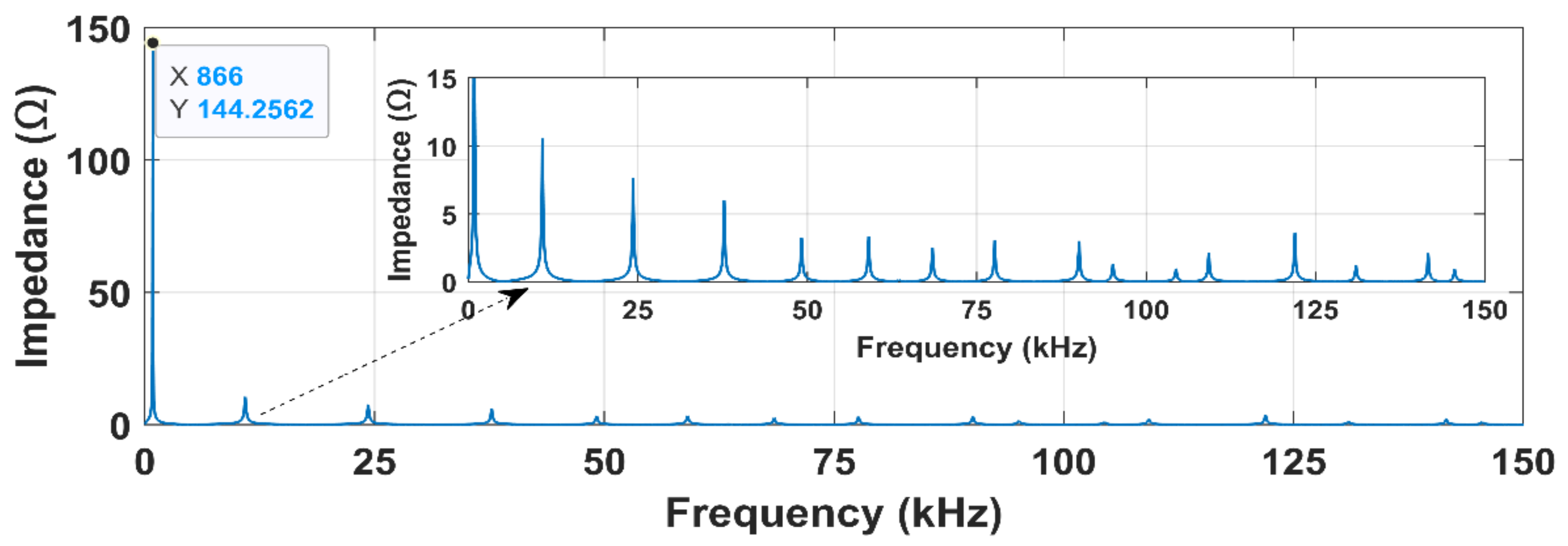
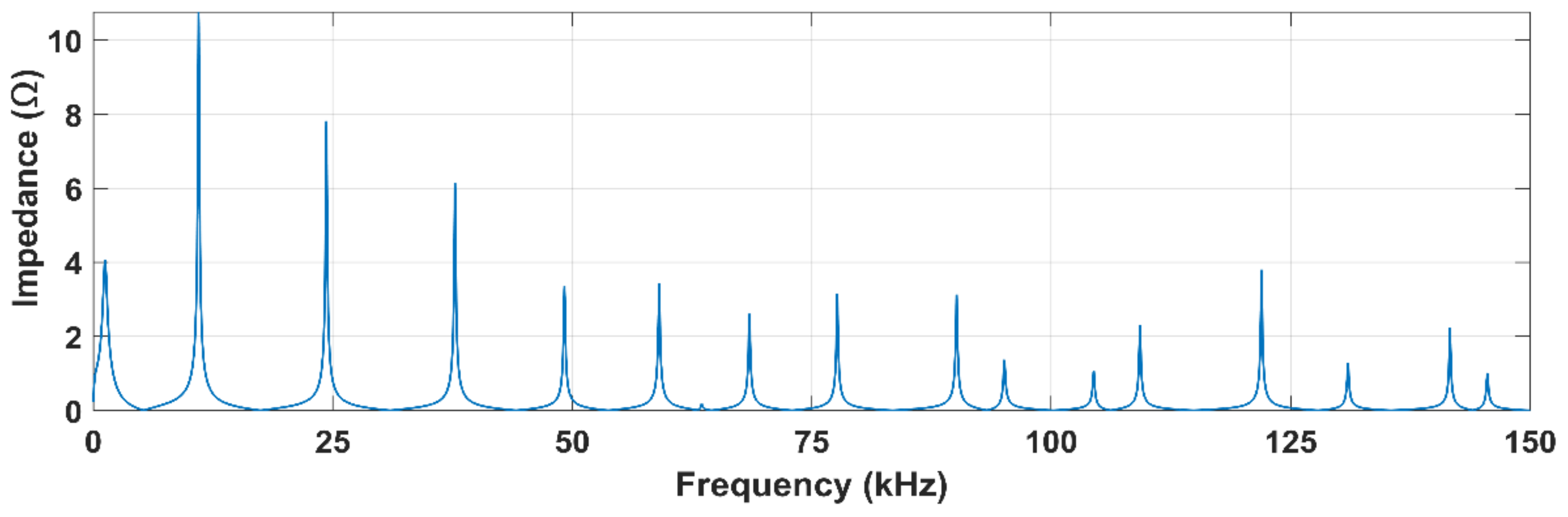
4.1.1. Feeder C Driving Point Impedance

The driving point impedance calculated at the nodes is obtained from the transfer function of the voltage output to the injected current input of the state space model. The node 1 impedance of the network shown in Figure 2 without feeder A and B, with all cables and transformers of feeder C, without any load connected to the distribution transformers has a resonance at 866 Hz, which corresponds well with the 871 Hz value obtained from the estimation. Though the first peak is below the supraharmonics range, it is relevant for other studies. It is included here for completeness. The medium voltage network also has a number of small resonance peaks between 2 and 150 kHz, as shown in Figure 3.

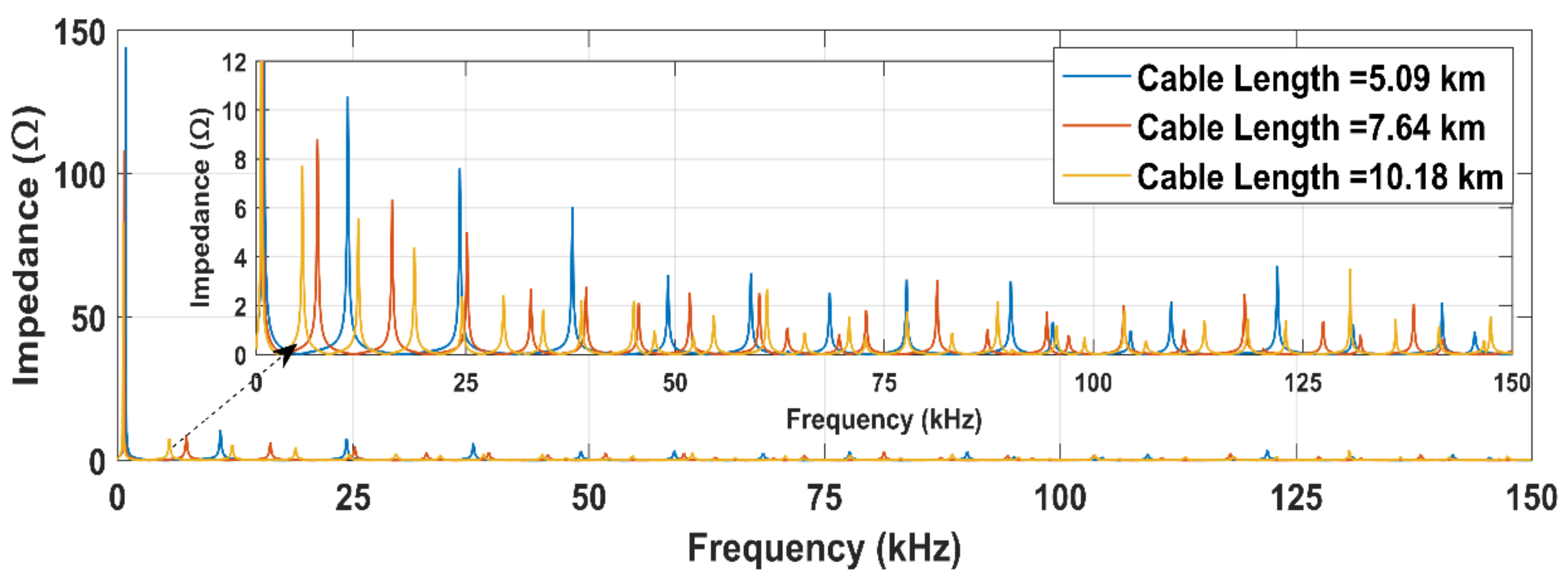
4.1.2. Impact of Cable Length

The total length of the cables of the system under study was 5.09 km. The impedance versus frequency of the system, with skin effect included, has been calculated when the length is increased to 1.5 and 2 times the original length. The results are shown in Figure 4. The magnitude of the impedance at the resonance frequency decreases with increase in cable length. Additionally, multiple resonances appear as the cable length increases; these are also shifted towards the lower frequency as shown in Figure 4.

4.1.3. Impact of Load Impedance

Considering maximum load values of 3.5 kW and 0.5 kVAR per LV customer obtained in consultation with field experts, the input impedance of the network with original length was again determined and the resulting resonances at 1255 Hz and 11 kHz are shown in Figure 5. It was shown earlier that the characteristic impedance of the lowest-frequency resonance corresponds to a load of 1400 kW. The load considered here is 272 times 3.5 kW or about 1000 kW, which is somewhat below the characteristic load. The impedance at the first resonance peak drops from over 144 Ω in Figure 3 to around 4 Ω in Figure 5. On the other hand, load has less impact on the supraharmonic frequencies.

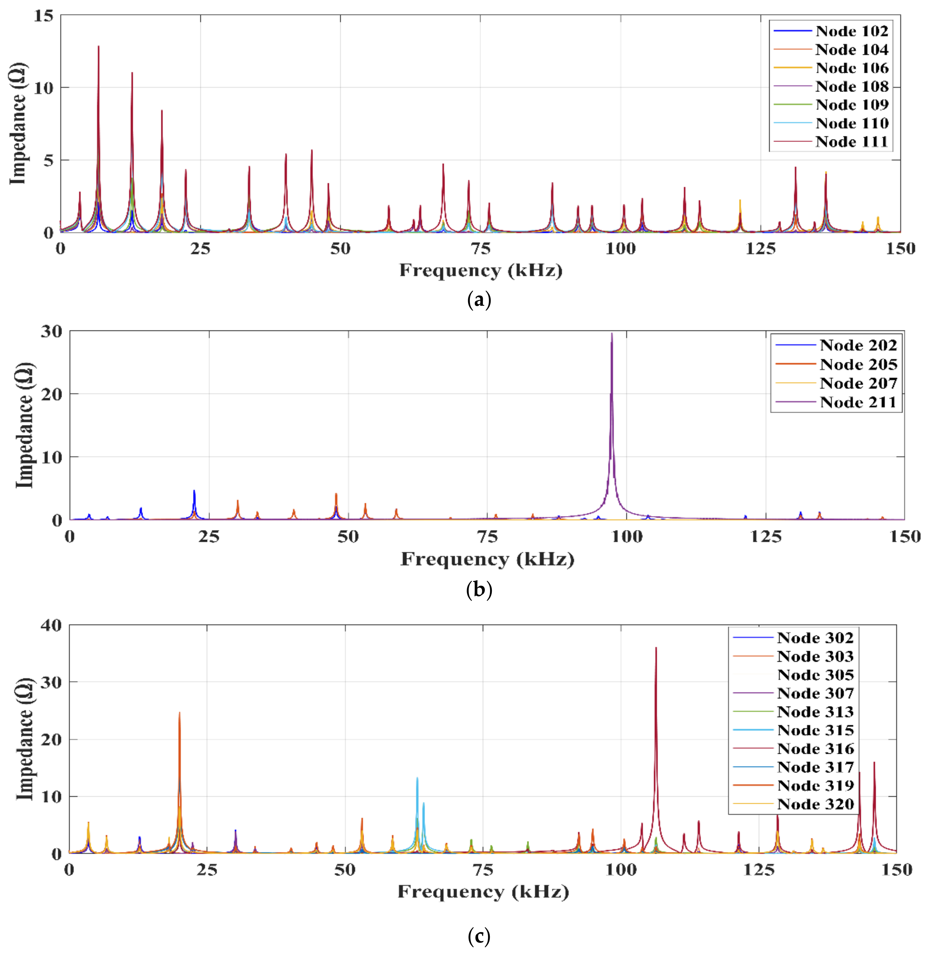
4.2. Feeder A, B and C Characteristics

In the previous section the characteristics of feeder C were analyzed in detail. In this section along with feeder C, feeder A and B are also connected as shown in Figure 3 and the characteristics of this combined configuration are studied. Magnitude of transfer impedance obtained using fast Fourier transform (FFT) analysis at the distribution transformer MV side by injecting a harmonic current at node 1 and node 214 is presented in

Table 4. Magnitude of transfer impedance obtained using FFT analysis.

Main Node (Point of Measurement)	Distance of Main Node from Point of Injection (Node 1) (km)	Distance of Main Node from Point of Injection (Node 214) (km)	Magnitude of 1 A, 12.8 kHz Harmonic Current Injected at Node 1	Magnitude of 1 A, 12.8 kHz Harmonic Current Injected at Node 214
			Transfer Impedance
			Ω	m Ω
Feeder A
102	0.368	4.82861	1.94	8.6
104	1.0931	5.55371	0.31	1.3
107	1.4166	5.87721	0.29	1.27
108	1.5804	6.04101	0.93	4.08
109	2.2534	6.71401	3.03	13.52
110	3.156	7.61631	4.87	21.72
111	3.6892	8.14981	5.19	22.94
Feeder B
202	0.43521	4.0253	2.2	9.82
205	1.19811	3.2624	0.8	3.6
207	1.58641	2.8741	0.0014	3.5 × 10−7
211	3.63501	1.2537	7.7 × 10−7	1.77 × 10−7
Feeder C
302	0.6442	5.10471	2.72	12.03
303	0.9589	5.41941	2.47	10.8
305	1.466	5.92651	1.61	7.1
307	1.8256	6.28611	0.77	3.3
313	3.2166	7.67711	1.69	7.3
315	3.2759	7.73641	1.61	7.31
316	3.1494	7.60991	1.47	7.1
317	2.9891	7.44961	1.72	8.46
319	3.4148	7.87531	1.79	8.69
320	3.7724	8.23291	1.66	7.6

.

Table 4 shows that the magnitude of transfer impedance initially decreases and further increases with increment in length and, in the case of Feeder C, it becomes almost constant towards the end of the feeder. Feeder B, with three wind turbines connected close to the node 214, shows a decreasing transfer impedance pattern.

The magnification of harmonic voltage at node 109, 110 and 111 towards the end of feeder A is noticeable. For a 1 A, 12.8 kHz (chosen based on the maximum resonance peak obtained using the combination of feeder A, B and C) supraharmonic current injection at node 1, node 109 generates 3 V, node 110 generates 4 V and Node 111 generates 5 V corresponding to a 10 kV system. The driving point impedance versus frequency at the MV side of the distribution transformer for feeder A, B and C is shown in Figure 6.

It is noticeable that the three feeders are rather similar in length and number of customers, but show big differences in the driving-point impedance.

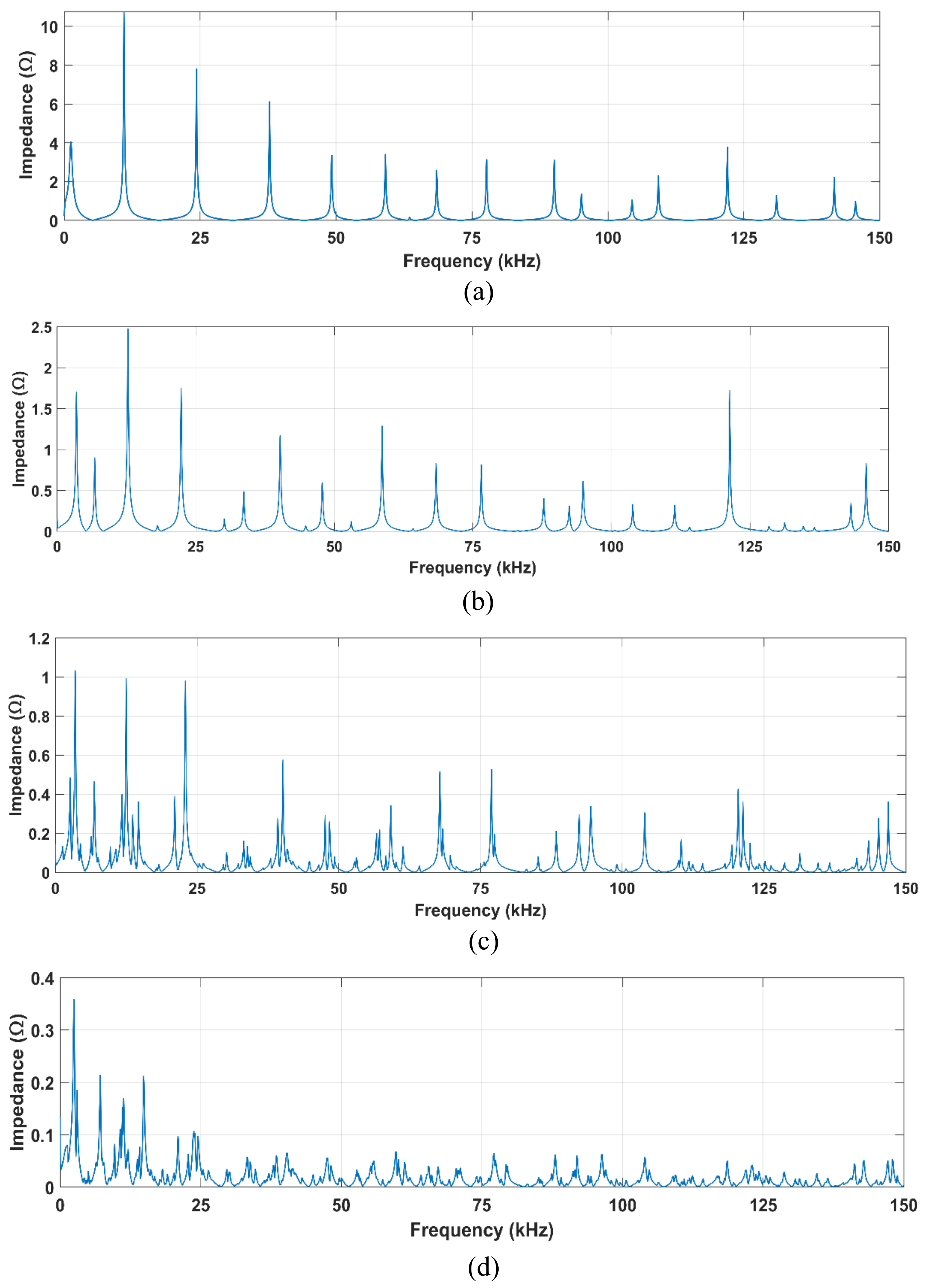
4.3. Feeders A,B,C,D,E,F,G and H Characteristics

In order to determine the input impedance of an MV network with eight feeders, four different configurations are studied by gradually increasing the number of feeders. Initially the input impedance of feeder C followed by feeder A, B and C followed by feeder A, B, C and D and finally all eight feeders are compared. All eight feeder details are given in Table 1. The input impedance obtained by a frequency scan at node 1 with four different feeder configurations with skin effect is shown in Figure 7.

The system impedance of feeder C is characterized by succession of parallel resonances over the range 0 to 150 kHz. As the number of feeders is increased, the magnitude of impedance decreases, and the number of resonance peaks increases as shown in Figure 7c,d.

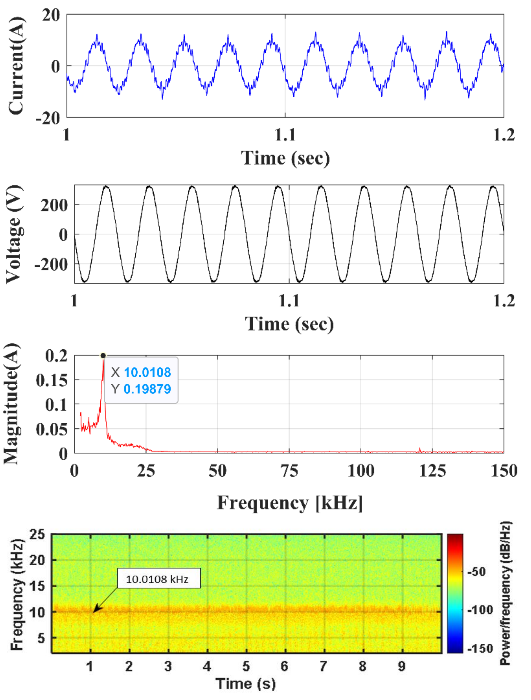
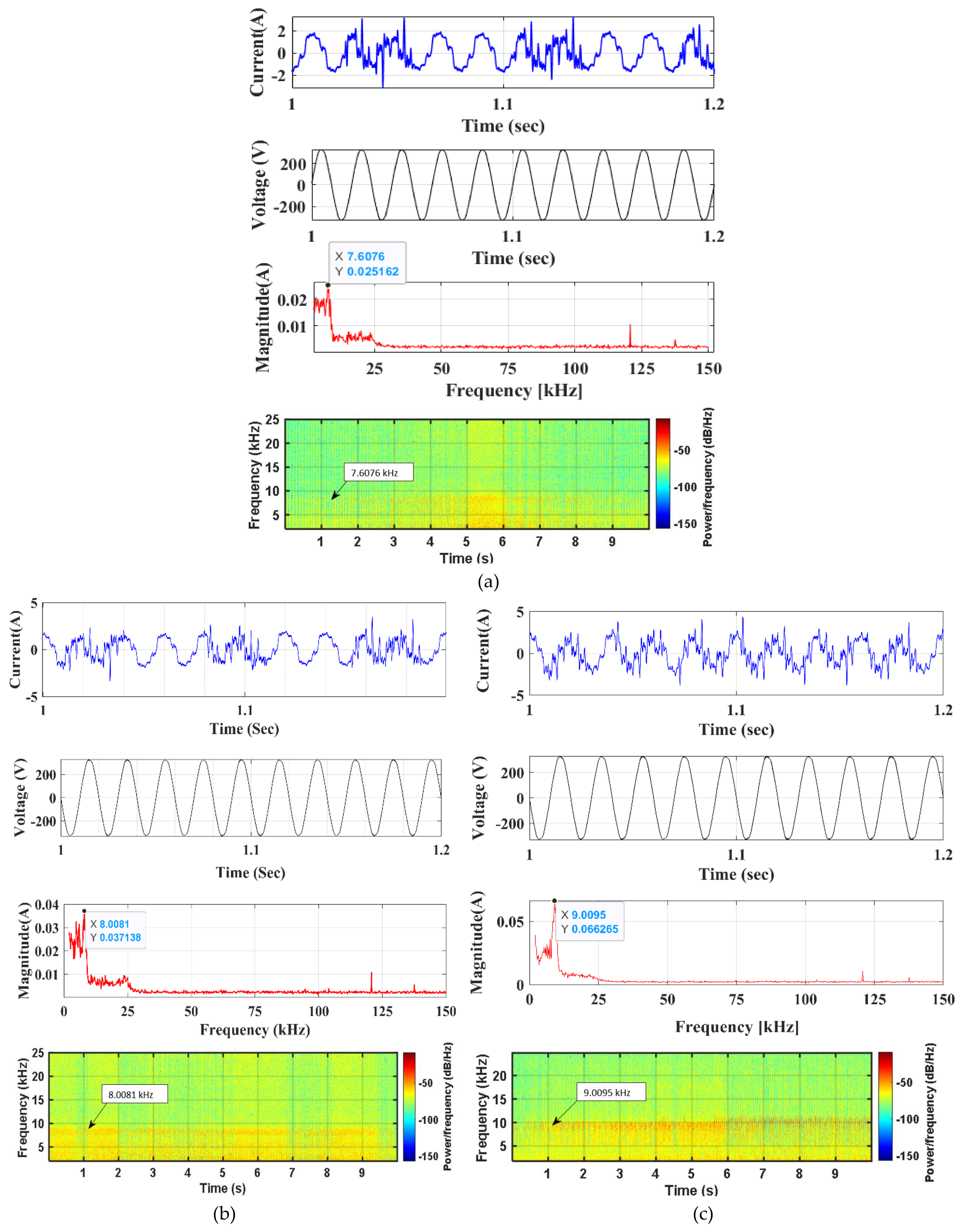
5. Supraharmonic Measurement at Feeder B

The power quality monitoring of a MV/LV network with 33 kV/11 kV transformer connected to eight different distribution feeders has been performed. Feeder B is connected to three wind turbines which cause the injection of supraharmonics into the MV network. A Hioki 8855 power quality monitor was used to acquire measurement data from the LV side of a 700 kVA transformer connecting a wind turbine. Pearson 411 current transformer with frequency resolution ranging from 1 Hz to 20 MHz was used. Different samples of data were acquired for 10 s at 5 min intervals with a sampling frequency of 500 kHz. The spectrum of voltage and current waveforms was obtained for 200 ms (10 cycles) using DFT with rectangular window. Hence, the frequency resolution of resulting spectra is 5 Hz. During normal operation of the converter, the switching frequency is 10 kHz, as shown in Figure 8.

To reduce the mechanical stress and increase the energy capture, a robust control scheme is used to control doubly fed induction generator (DFIG) based wind turbines [31,32]. During low power extraction, a time varying emission due to the variation of the switching frequency of the wind turbine at different operating modes of the converter was observed. Switching frequencies were ranging from 7 to 10 kHz. Switching frequencies of 7.6, 8 and 9 kHz during low active power generation are shown in Figure 9.

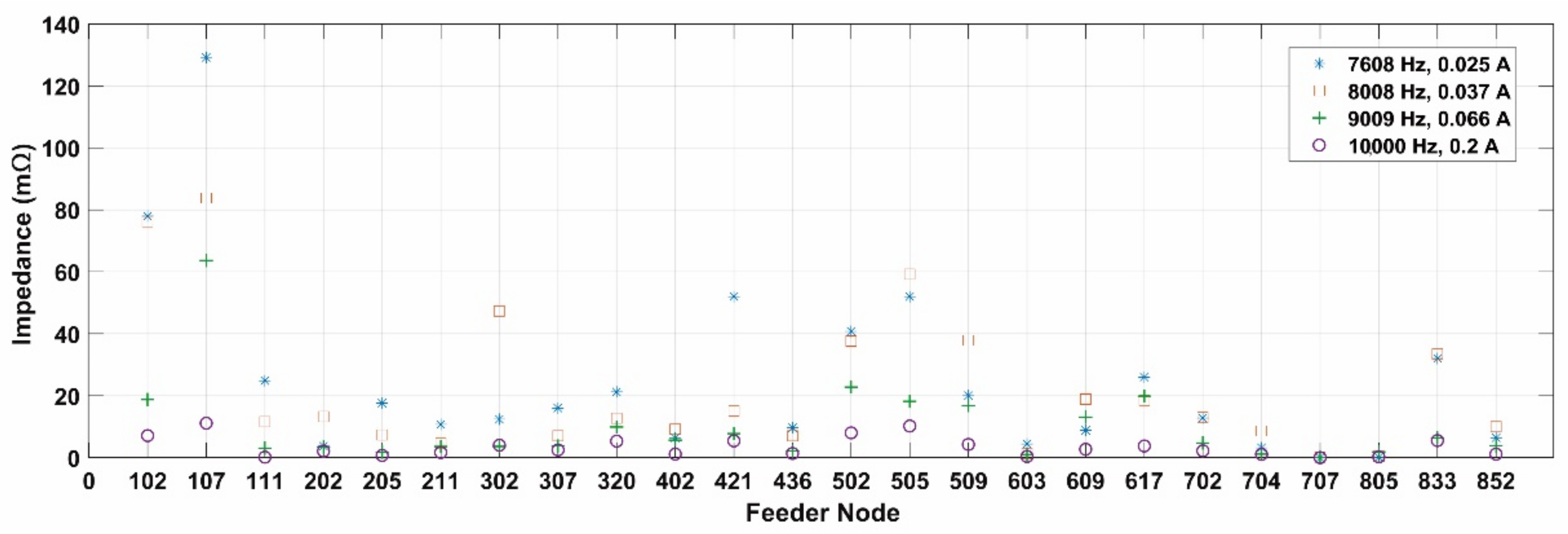
6. Transfer Impedance Estimation

The supraharmonic emissions of 10 kHz, 0.2 A, 9 kHz, 0.066 A, 8 kHz, 0.037 A and 7.6 kHz, 0.025 A, observed in the measurements, injected by the wind turbines at PCC, have been used for further analysis. These supraharmonic currents were injected into the MV side of the wind turbine transformer at node 214 (point of connection of wind turbines) of the developed MATLAB model with all eight feeders. The transfer impedance is obtained as a ratio of the voltages developed at selected nodes of different feeders to the injected supraharmonic current. The transfer impedance measurement as a function of frequency is obtained at the MV side of selected distribution transformers (selected based on the distance from the main 33 kV/11 kV transformer) of all eight feeders as shown in Figure 10. It is noticed that the transfer impedance value decreases for short feeders and for further increment in length of the feeder the transfer impedance increases. For very long feeders it again starts decreasing towards the end of the feeder.

To determine how severe these impedance values are, let us consider that the 700 kVA wind turbine in feeder B injects 1% supraharmonic current at the resonance frequency. The rating, 700 kVA, 10 kV, corresponds to 40 A rated current; hence 1% supraharmonic current is 0.4 A. Assuming a transfer impedance of 130 mΩ at node 107 of feeder A, 0.4 A gives a voltage of 0.052 V, which is a very small value of the nominal phase-to-neutral voltage. Hence it can be concluded that the transfer impedance values are very small in the medium voltage network with all eight feeders under study and it does not create much impact on the grid. On the other hand, with three feeder configuration in Section 4.2 the node 111 was capable of generating 5 V under the influence of supraharmonic current of 1 A, 12.8 kHz.

The 5 V generated by the supraharmonics current of 1 A is plotted with respect to the EN50160 standard voltage limits for frequency range 95 kHz upto 148.5 kHz used in public LV and MV network [2]. Voltage level in % for 5 V corresponding to 10 kV is 0.05% which is within the standards as shown in Figure 11. If aggregation of supraharmonics generated by multiple devices get amplified by resonance and generate 50 V it would cross the EN50160 standard. The limits according to EN50065 and IEC 61000-3-8 is only 2% of nominal voltage for the frequency range between 3 and 9 kHz [2]. In this case an aggregation of 20 V in the 10 kV network will cross the IEC standard limit. Hence advance study on different network configurations with large numbers of power converters and their aggregation in the supraharmonics range are essential. This would help the standardization committee to fix the new equipment’s emission limit in the supraharmonics range during their testing. It should be noted that all limits in this frequency range was fixed based on power line communication apparatus, hence the limits need to be redefined based on the modern power system requirements.

7. Conclusions

The emission limits for higher frequencies (2 kHz–150 kHz) are of interest among different standardization group. The lack of knowledge about the transfer impedance of the MV network in the supraharmonics frequency range has set limitations to define standards/immunity limits for power converters based supraharmonic sources integrated to the grid.

This work has studied the propagation of supraharmonics in specific MV\LV power grid network configurations. Thereafter, supraharmonic voltages were estimated from measurement and the simulated characteristics of the MV network. The general findings after analyzing the existing MV\LV Swedish network with eight feeders can be summarized as follows:

• The first resonance in the MV network is mainly due to the source and transformer inductance together with the total cable capacitance.
• In the MV network, there are large number of resonances in the supraharmonic frequency range.
• The skin effect provides significant damping, but resonance peaks remain sharp within the supraharmonic frequency range.
• The bigger the MV network, the more resonance frequencies, but also the lower the amplitude of the resonance peaks.
• Measurements close to a wind turbine converter show a time varying emission in the supraharmonics range due to the variation in switching frequency of the wind turbine converter at different operating modes during low power extraction.
• For short feeders as length increases, the magnitude of the transfer impedance at supraharmonic frequency decreases. For further increment in feeder length, the magnitude increases or becomes almost constant. For very long feeders the transfer impedance starts decreasing further.

The amplification of supraharmonics in a network configuration with fewer feeders was high as discussed in Section 4.2. This study helps to better understand the propagation of supraharmonic resonances in MV\LV networks. With the conclusions of this work and the knowledge about the transfer impedance and resonant peaks in the MV network the possible amplification and expected levels of these emissions in the grid can be predicted. Hence, this study would help standardization committee to set compatibility levels or emission limits for these non-intentional emissions in the MV network. The study can be extended to investigate the aggregation of supraharmonic emission in the MV network due to interaction of multiple sources of supraharmonic emissions. Further research could investigate the fault tripping of protection system due to amplified supraharmonics.

References

1. Rönnberg, S.K.; Bollen, M.H.; Amaris, H.; Chang, G.W.; Gu, I.Y.; Kocewiak, Ł.H.; Meyer, J.; Olofsson, M.; Ribeiro, P.F.; Desmet, J. On waveform distortion in the frequency range of 2 kHz–150 kHz—Review and research challenges. Electr. Power Syst. Res. 2017, 150, 1–10. [Google Scholar] [CrossRef]
2. Bollen, M.; Olofsson, M.; Larsson, A.; Ronnberg, S.; Lundmark, M. Standards for supraharmonics (2 to 150 kHz). IEEE Electromagn. Compat. Mag. 2014, 3, 114–119. [Google Scholar] [CrossRef]
3. Rönnberg, S.K.; Bollen, M.H.J. Propagation of Supraharmonics in the Low Voltage Grid 2 to 150 kHz; Electra Program and Swedish Energy Agency Report; Energiforsk: Stockholm, Sweden, December 2017; ISBN 978-91-7673-461-2. [Google Scholar]
4. Sakar, S.; Rönnberg, S.K.; Bollen, M.H.J. Interferences in AC–DC LED drivers exposed to voltage disturbances in the fre-quency range 2–150 kHz. IEEE Trans. Power Electron. 2019, 34, 11171–11181. [Google Scholar] [CrossRef]
5. Paulsson, L.; Ekehov, B.; Halen, S.; Larsson, T.; Palmqvist, L.; Edris, A.-A.; Kidd, D.; Keri, A.; Mehraban, B. High-frequency impacts in a converter-based back-to-back tie; the eagle pass installation. IEEE Trans. Power Deliv. 2003, 18, 1410–1415. [Google Scholar] [CrossRef]
6. Kalesar, B.M.; Noshahr, J.B. Capacitor bank behaviour of cement factory in presence of supraharmonics resulted from switching full power frequency converter of generator (PMSG). In Proceedings of the 24th International Conference on Electricity Distribution, Glasgow, UK, 12–15 June 2017. [Google Scholar]
7. Yalcin, T.; Ozdemir, M.; Kostyla, P.; Leonowicz, Z. Analysis of supra-harmonics in smart grids. In Proceedings of the 2017 IEEE International Conference on Environment and Electrical Engineering and 2017 IEEE Industrial and Commercial Power Systems Europe (EEEIC/I&CPS Europe), Milan, Italy, 6–9 June 2017; pp. 1–4. [Google Scholar]
8. Slangen, T.; Van Wijk, T.; Ćuk, V.; Cobben, S. The Propagation and Interaction of Supraharmonics from Electric Vehicle Chargers in a Low-Voltage Grid. Energies 2020, 13, 3865. [Google Scholar] [CrossRef]
9. Rönnberg, S.K. Emission and Interaction from Domestic Installations in the Low Voltage Electricity Network, up to 150 kHz. Ph.D. Thesis, Luleå University of Technology, Luleå, Sweden, 2013. [Google Scholar]
10. Larsson, A. On High-Frequency Distortion in Low-Voltage Power Systems. Ph.D. Thesis, Luleå University of Technology, Luleå, Sweden, 2011. [Google Scholar]
11. Klatt, M.; Meyer, J.; Schegner, P.; Koch, A.; Myrzik, J.; Eberl, G.; Darda, T. Emission levels above 2 kHz—Laboratory results and survey measurements in public low voltage grids. In Proceedings of the 22nd International Conference and Exhibition on Electricity Distribution (CIRED 2013), Stockholm, Sweden, 10–13 June2013. [Google Scholar]
12. Espín-Delgado, Á.; Rönnberg, S.; Busatto, T.; Ravindran, V.; Bollen, M. Summation law for supraharmonic currents (2–150 kHz) in low-voltage installations. Electr. Power Syst. Res. 2020, 184, 106325. [Google Scholar] [CrossRef]
13. Rönnberg, S.K.; Bollen, M.H.J.; Larsson, A.; Lundmark, M. An Overview of the Origin and Propagation of Supraharmonics (2–150 kHz. In Proceedings of the Nordic Conference on Electricity Distribution System Management and Development, Stockholm, Sweden, 8–9 September 2014. [Google Scholar]
14. Matthias, K.; Kaiser, F.; Meyer, J.; Lakenbrink, C.; Gassner, C. Measurements and simulation of supraharmonic resonances in public low voltage networks. In Proceedings of the 25th International Conference on Electricity Distribution, Madrid, Spain, 3–6 June 2019. [Google Scholar]
15. Ma, Z.; Xu, Q.; Li, P.; Wu, J.; Huang, H. Supraharmonics Analysis of Modular Multilevel Converter and Long Cable System. In Proceedings of the 2019 IEEE Sustainable Power and Energy Conference (iSPEC), Beijing, China, 21–23 November 2019; pp. 2585–2589. [Google Scholar]
16. Noshahr, J.B. Emission phenomenon of supra-harmonics caused by switching of full-power frequency converter of wind turbines generator (PMSG) in smart grid. In Proceedings of the 2016 IEEE 16th International Conference on Environment and Electrical Engineering (EEEIC), Florence, Italy, 7–10 June 2016; pp. 1–6. [Google Scholar]
17. Blanco, A.M.; Heimbach, B.; Wartmann, B.; Meyer, J.; Mangani, M.; Oeschger, M. Harmonic, interharmonic and suprahar-monic characterisation of a 12 MW wind park based on field measurements. CIRED-Open Access Proc. J. 2017, 677–681. [Google Scholar] [CrossRef] [Green Version]
18. Mohos, A.; Ladanyi, J. Emission Measurement of a Solar Park in the Frequency Range of 2 to 150 kHz. In Proceedings of the 2018 International Symposium on Electromagnetic Compatibility (EMC EUROPE), Amsterdam, The Netherlands, 27–30 August 2018; pp. 1024–1028. [Google Scholar] [CrossRef]
19. Mumtaz, M.; Khan, S.I.; Chaudhry, W.A.; Khan, Z.A. Harmonic incursion at the point of common coupling due to small grid-connected power stations. J. Electr. Syst. Inf. Technol. 2015, 2, 368–377. [Google Scholar] [CrossRef] [Green Version]
20. Rönnberg, S.K.; Castro, A.G.; Bollen, M.H.J.; Moreno-Munoz, A.; Romero-Cadaval, E. Supraharmonics from power elec-tronics converters. In Proceedings of the 9th International Conference on Compatibility and Power Electronics (CPE), Costa da Caparica, Lisbon, Portugal, 24–26 June 2015; pp. 539–544. [Google Scholar]
21. Gil-de Castro, A.; Moreno-Munoz, A.; Garrido, J.; Rönnberg, S.K.; Palacios-Garcia, E.J.; Morales, T. Supraharmonics reduc-tion in NPC inverter with random PWM. In Proceedings of the 2017 IEEE 26th International Symposium on Industrial Electronics (ISIE), Edinburgh, UK, 19–21 June 2017; pp. 1792–1797. [Google Scholar]
22. Novitskiy, A.; Schlegel, S.; Westermann, D. Analysis of supraharmonic propagation in a MV electrical network. In Proceedings of the 2018 19th International Scientific Conference on Electric Power Engineering (EPE), Brno, Czech Republic, 16–18 May 2018; pp. 1–6. [Google Scholar]
23. Novitskiy, A.; Schlegel, S.; Westermann, D. Measurements and analysis of supraharmonic influences in a MV/LV network containing renewable energy sources. In Proceedings of the 2019 Electric Power Quality and Supply Reliability Conference (PQ) & 2019 Symposium on Electrical Engineering and Mechatronics (SEEM), Kärdla, Estonia, 12–15 June 2019. [Google Scholar]
24. Bengtsson, T.; Dijkhuizen, F.; Ming, L.; Sahlen, F.; Liljestrand, L.; Bormann, D.; Papazyan, R.; Dahlgren, M. Repetitive fast voltage stresses-causes and effects. IEEE Electr. Insul. Mag. 2009, 25, 26–39. [Google Scholar] [CrossRef]
25. Espín-Delgado, A.; Letha, S.S.; Rönnberg, S.K.; Bollen, M.H.J. Failure of MV cable terminations due to supraharmonic volt-ages: A risk indicator proposal. IEEE Open J. Ind. Appl. 2020, 1, 42–51. [Google Scholar] [CrossRef]
26. Espín-Delgado, A.; Letha, S.S.; Rönnberg, S.K.; Bollen, M.H.J. Indicators for supraharmonics based on their impact on end-User equipment. Unpublished.
27. Bollen, M.; Mousavi-Gargari, S.; Bahramirad, S. Harmonic resonances due to transmission-system cables. Renew. Energy Power Qual. J. 2014, 712–716. [Google Scholar] [CrossRef]
28. Dommel, H. Digital computer solution of electromagnetic transients in single and multiple networks. IEEE Trans. Power App. Syst. 1969, PAS-88, 388–399. [Google Scholar] [CrossRef]
29. Corcoran, J.; Nagy, P.B. Compensation of the Skin Effect in Low-Frequency Potential Drop Measurements. J. Nondestruct. Eval. 2016, 35, 58. [Google Scholar] [CrossRef] [Green Version]
30. Wiring Systems for Max 1000 V—Methods of Calculation to Safeguard Correct Disconnection; Svensk Standard SS 424 14 05; SEK Swedish Electricity Standard: Kista, Sweden, 1993.
31. Beltran, B.; Benbouzid, M.E.H.; Ahmed-Ali, T. Second-order sliding mode control of a doubly fed induction generator driv-en wind turbine. IEEE Trans. Energy Convers. 2012, 27. [Google Scholar] [CrossRef] [Green Version]
32. Luo, N.; Vidal, Y.; Acho, L. (Eds.) Wind Turbine Control and Monitoring Advances in Industrial Control; Springer: Berlin/Heidelberg, Germany, 2014; p. 466. ISBN 3319084135. [Google Scholar]
Figure 1. Two port network of distributed parameter transmission line model.
Energies 14 01093 g001
Figure 2. Single line diagram of feeder A, B and C with 272 customers.
Energies 14 01093 g002
Figure 3. Frequency response without load.
Energies 14 01093 g003
Figure 4. Frequency response at different cable length.
Energies 14 01093 g004
Figure 5. Frequency response with load.
Energies 14 01093 g005
Figure 6. Driving point impedance of test network at medium voltage (MV) side of distribution transformer (a) feeder A, (b) feeder B and (c) feeder C.
Energies 14 01093 g006
Figure 7. MV network impedance at node 1 (a) feeder C, (b) feeder A, B and C, (c) feeder A, B, C and D and (d) feeder A, B, C, D, E, F, G and H. Note the difference in vertical scale between.
Energies 14 01093 g007
Figure 8. Transformer MV side current and voltage waveforms along with its spectrum with dominant emission at 10 kHz at PCC of wind turbines of feeder B.
Energies 14 01093 g008
Figure 9. Transformer MV side current and voltage waveforms along with its dominant emission at (a) 7.6, (b) 8 and (c) 9 kHz at PCC of wind turbines of feeder B.
Energies 14 01093 g009
Figure 10. Transfer Impedance at different nodes of the MV network for supraharmonic current injection.
Energies 14 01093 g010
Figure 11. Emission limits at supraharmonics frequency range as per standards.
Energies 14 01093 g011